Reduction Mappings between Probabilistic
Boolean Networks
Ivan Ivanov
Department of Electrical Engineering, Texas A&M University, College Station, TX 77843, USA Email:[email protected]
Edward R. Dougherty
Department of Electrical Engineering, Texas A&M University, 3128 TAMU College Station, TX 77843-3128, USA Email:[email protected]
Received 11 April 2003; Revised 28 August 2003
Probabilistic Boolean networks (PBNs) comprise a model describing a directed graph with rule-based dependences between its nodes. The rules are selected, based on a given probability distribution which provides a flexibility when dealing with the uncer-tainty which is typical for genetic regulatory networks. Given the computational complexity of the model, the characterization of mappings reducing the size of a given PBN becomes a critical issue. Mappings between PBNs are important also from a theoretical point of view. They provide means for developing a better understanding about the dynamics of PBNs. This paper considers two kinds of mappings reduction and projection and their effect on the original probability structure of a given PBN.
Keywords and phrases:Boolean network, genetic network, graphical models, projection, reduction.
1. INTRODUCTION
Given a set of genes, the evolution of their expressions consti-tutes a dynamical system over time. Owing to the complexity of gene interaction and the paucity of data, homogeneous transitions are customarily assumed. Many different gene-regulatory-network models have been proposed. Among de-terministic dynamical systems, perhaps, the most attention has been given to the Boolean network model [1,2,3]. In this model, gene expression is quantized to only two levels: ON and OFF. The expression level (state) of a gene is func-tionally related, via a logical rule, to the expression states of some other genes. The Boolean network model has yielded insights into the overall behavior of large genetic networks [4,5,6,7], thereby facilitating the study of large data sets in a global fashion. Here, we are concerned with a stochas-tic extension of the Boolean model that results in probabilis-tic Boolean networks [8,9]. For these, similarities exist with Bayesian networks [10,11,12,13] and, more generally, with models including stochastic components on the molecular level [14,15,16].
The dynamical behavior of such networks can be used to model many biologically meaningful phenomena—for in-stance, cellular state dynamics, possessing switch-like be-havior, stability, and hysteresis [17]. Besides the conceptual framework offered by such models, there are practical uses,
such as the identification of suitable drug targets in cancer therapy or inferring the structure of the genetic models from experimental data, for example, from the gene expression profiles [17]. To that end, a significant effort has gone into identifying the structure of gene regulatory networks from expression data [8,18,19,20,21,22,23].
Probabilistic Boolean networks (PBNs) [8,9] constitute a probabilistic generalization of Boolean networks and of-fer a more powerful and flexible modeling framework. They share the appealing rule-based properties of the Boolean net-works, are robust to uncertainty both in the data and model selection, and can be studied in the probabilistic context of Markov chains (see also [23]). PBNs enable the systematic study of global network dynamics and permit quantification of the relative influence and sensitivity of genes in their in-teractions with other genes. While the Boolean assumption is useful for a simple up- or down-regulated model and also useful for reducing the complexity of the network, the ba-sic model extends directly to a finite-state-space model, and inference has been studied in that context in [22].
of a particular gene from ON to OFF or vice versa to facil-itate the transition to some other desirable state or set of states. Specifically, using the concept of the mean first pas-sage time, it has been demonstrated how the particular gene, whose transcription status is to be momentarily altered to initiate the state transition, can be chosen to “minimize” (in a probabilistic sense) the time required to achieve the desired state transitions [24]. A second approach has aimed at chang-ing the steady-state (long-run) behavior of the network by minimally altering its rule-based structure [25]. A third ap-proach has focused on applying ideas from control theory to develop an intervention strategy in the general context of Markovian genetic regulatory networks whose state transi-tion probabilities depend on an external (control) variable [26].
An obstacle in applying PBNs is the computational com-plexity of the model. Owing to the large number of states often present in full networks, it is sometimes necessary to construct computationally tractable subnetworks while still carrying sufficient structure for the application at hand— hence, the need for size reducing mappings between PBNs. Construction of mappings to alter PBN structure while at the same time maintaining consistency with the original prob-ability structure have previously been studied [27]. These include projections onto subnetworks. Unfortunately, while projections maintain the probabilistic structure by reduc-ing the number of genes, they also increased the complex-ity of the Boolean function structure. This paper considers reduction mappings of a PBN that alter the structure of the network while maintaining maximum consistency with the original probability structure. Once this notion of maximum consistency has been defined, the problem reduces to one of optimization. Thus, a key issue to be addressed in this paper is the positing of consistency conditions.
2. DEFINITIONS AND BASIC PROPERTIES
This section provides the definitions and the basic proper-ties of probabilistic Boolean networks as given in [8]. While there have been some generalization of the model [9,24], we stay with the original definition, as has the original analysis of projection mappings between PBNs [27]—which plays a key role in the present paper. A PBN (V,F,C) is defined by a set of nodes (genes)
V =x1,. . .,xn
,
xi∈ {0, 1},
i=1,. . .,n,
(1)
a list of predictors
F=F1,. . .,Fn
,
Fi=
f1(i),. . .,fl(i)(i)
,
fj(i):{0, 1}n−→ {0, 1},
(2)
and a list
C=C1,. . .,Cn,
Ci=
c(i) 1 ,. . .,c
(i) l(i)
(3)
of selection probabilitiesc(ji) =Pr{f(i) = f(i)
j }with respect to a list (vector) of probability distributions (ν(1),. . .,ν(n)), wheref=(f(1),. . .,f(n)) is a random vector taking values in
F. Each nodexirepresents the state (expression) of the gene
i, wherexi = 0 means that the geneiis not expressed and
xi = 1 means that it is expressed. Every setFi contains the possible rules fj(i) of regulatory interactions for the genei. These functions are also calledpredictorsfor the correspond-ing gene. Updatcorrespond-ing of the states of all genes in the network is done synchronously according to the functions assigned to the genes, and then the process is repeated. The predic-tors for every gene xi are selected simultaneously and ran-domly (according to the listC) from the setsFiat every time step.
Arealizationof a PBN is determined at every time step by the vector f. If the predictor for each gene is chosen in-dependently of the other predictors, then the number of all possible realizationsfk=(fk(1)1 ,. . .,fk(n)n ),k=1,. . .,N, of the PBN isN=nj=1l(j). Even though the domain of every pre-dictor fj(i)is assumed to be{0, 1}n, there are only a few input genes that actually regulate xi at any given time step. This simplification can be justified by some biological and practi-cal considerations [8]. In general, there is no need of the as-sumption that f(1),f(2),. . .,f(n)are selected independently; however we make this assumption. A PBN that satisfies this assumption is calledindependent. For an independent PBN, we have
Pk=Prf=fk= n
j=1
Prf(i)= fk(i)j =n
j=1c (i) kj. (4)
In [8], the listCof selection probabilities is created using the
coefficient of determination[28,29].
A PBN can be interpreted as a homogeneous Markov chain relative to the statesx=(x1,x2,. . .,xn) of the network with transition probabilities given by
Prx−→x=
i
Pi, (5)
where the summation is over the indices i such that i :
fK(i)i1(x1,. . .,xn) = x1,. . .,fK(n)in(x1,. . .,xn) = xnandK is the matrix with rows given by the possible realizations of the PBN [8].
3. PBN PROJECTION MAPPING
transforms the given PBN into a new one, where the num-ber of the genes is reduced by one, that is, the genexiin the original network is “deleted.” Without loss of generality, we may assume that the deleted gene is the last one,xn. Thus,
Πn:A→Aˆ, ˆA( ˆV, ˆF, ˆC), where ˆ
V=x1,. . .,xn−1, Fˆ=Fˆ1,. . ., ˆFn−1, ˆ
C=Cˆ1,. . ., ˆCn−1. (6)
Every ˆFiand every ˆCihave twice as many elements as the cor-responding setsFiandCiinA. Every predictor fj(i)∈Fi gen-erates two predictors ˆf0(ij)and ˆf1(ji)according to the rule
ˆ
fk j(i)x1,. . .,xn−1=fj(i)x1,. . .,xn−1,k, (7)
wherek∈ {0, 1}and (x1,. . .,xn−1) is in ˆA. The new Boolean functions ˆfk j(i),k=0, 1, have transition probabilities
ˆ
ck j(i)=c(i)j Prxn=k, k∈ {0, 1}. (8) It is noticed in [27] that there is a difficulty in defining the new selection probabilities ˆck j(i) because the probabilities for the genexndepend on the current state probability distribu-tion of the underlying Markov chain. One way to go around the problem is to use the steady state distribution forAor, the stationary distribution forAif there is no steady state distri-bution. Another way is to estimate Pr{xn=k},k =0, 1, by runningAfor some time. In doing so, one has to be aware of the possible transient behavior of those probabilities. Yet, another way to find the values of Pr{xn=k}is to use the data set from which the original PBNAwas created.
4. PBN REDUCTION MAPPINGS
In this paper, we propose a new kind of mapping that also reduces the size of a given PBN. In contrast to the projection mapping discussed in the previous section, this new mapping does not increase the number of the predictors for the genes that remain in the new network. One has to keep in mind that any such mapping might not preserve the probability structure of the original PBN. For example, this will be the case if the deleted gene isessentialfor one of the predictors of the remaining genes [8].
Therefore, the problem is to find a reduction mapping that renders a PBN close to the original one. To be more spe-cific, consider an independent PBNA(V,F,C) and a map-pingπn:A→A˜, ˜A( ˜V, ˜F, ˜C), where
˜
V=x1,. . .,xn−1
, F˜=F˜1,. . ., ˜Fn−1
, ˆ
C=Cˆ1,. . ., ˆCn−1, (9)
where ˜A( ˜V, ˜F, ˜C) is an independent PBN with ˜Fi =
{f˜(i) 1 ,. . ., ˜f
(i)
l(i)}, ˜fj(i):{0, 1}n−1 → {0, 1}, and ˜c(ji)=Pr˜{f˜(i)= ˜
fj(i)} with respect to some probability distribution vector (˜ν(1),. . ., ˜ν(n−1)). Note that the cardinality of ˜Fi is the same as the cardinality ofFi. The new PBN ˜Ais called areduced
PBN obtained from the original PBN Aby deleting one of the genes inA. As inSection 3, we have assumed without loss of generality that the deleted gene isxn.
The reductionπnshould yield a PBN that is “close” to the original, and there are various natural ways to interpret this closeness:
(A) for every ˜c(i)j ,|c˜(i)j −c(i)j | ≤for some given≥0; (B) the transition probabilities for the state diagrams ofA
and ˜Aare close;
(C) the stationary/steady-state distributionsDofAand ˜D of ˜Aare close;
(D) every new predictor function ˜fj(i)is selected as close as possible to both functions ˆfk j(i),k = 0, 1, given by the projected PBN ˆA.
Some comments about the preceding conditions are in order.
(A) In the context of gene regulatory networks, one can expect the numberto be reasonably small, and per-haps even equal to zero, that is, the predictors for the genes in the reduced PBN ˜Ahave the same selection probabilities as their corresponding predictors from the original PBNA.
(B) Consider the portion of the state diagram ofA con-taining the statesi1 = (x1,. . .,xn−1, 1),i0 = (x1,. . .,
xn−1, 0),j1=(x1,. . .,xn−1 , 1), andj0=(x1,. . .,xn−1, 0):
i1
pi1j1
j1
pi1j0
pi0j1
i0 pi0j0 j0
wherepi1j1,pi0j0,pi1j0, andpi0j1are the corresponding transition probabilities. If one “deletes” the nodexn, this diagram collapses to the following one:
i p
∗ ij
j
wherei=(x1,. . .,xn−1) andj =(x1,. . .,xn−1) are the corresponding states in ˜A, and
p∗ ij=Pr
xn=1pi1j1+pi1j0
+ Prxn=0pi0j1+pi0j0
. (10)
The transition probabilities for the reduced PBN ˜Aare given by (see [8])
˜
pij= i
˜
Pi, (11)
where the summation is over the indicesisuch thati: ˜
Since the transition probability matrices forAand ˜A have different dimensions, one cannot compare them directly. This is why we compare the ˜pij’s to thepij∗’s, and the term “close” in part (B) refers to the quantity maxi,j|p˜ij−pij∗|being small.
(C) Collapsing the state transition diagram, as described in part (B), induces a probability distributionD∗on the state space of ˜Ain the following way:
Pr∗state in ˜A=x1,. . .,xn−1
=Prstate inA=x1,. . .,xn−1, 0 + Prstate inA=x1,. . .,xn−1, 1
.
(12)
Notice that one cannot compare the distributionDto the distribution ˜D directly because they are defined over different state spaces. This is why the term “close” in (C) refers to the closeness of the distributionD∗and the stationary state distribution ˜Dof ˜Ain thel1sense, that is, to the quantity
D∗−D˜ l1=
˜
x∈S˜
Pr∗{x} −Pr˜{x} (13)
being small. Here, ˜S= {0, 1}n−1is the set of all states in ˜A, and ˜Pr is associated with ˜D.
(D) Using the notation from (D), we have the following proposition.
Proposition 1. Given a PBNAwith a stationary state distri-butionD, consider the projected PBNAˆ. Then
ED
∂ fj(i)
∂xn
=fˆ(i)
0j −fˆ1j(i)l2n−1 1
=ED∗fˆ0j(i)−fˆ1(i)j
. (14)
Here the spacel12n−1 is endowed with the probability measure ˜
Prdefined by the distributionD∗, andED means the expecta-tion of the corresponding random variable with respect to the distributionD.
Proof. The claim in this proposition becomes obvious if one notices that for every state (x1,. . .,xn−1,xn) ∈ {0, 1}n, where ∂ fj(i)/∂xn=1, there are two terms in the sum that compute ED(∂ fj(i)/∂xn), namely, Pr{(x1,. . .,xn−1, 0)} and Pr{(x1,. . .,xn−1, 1)}.
The proposition plays an important role in selecting the new predictor function ˜fj(i). Notice that the expectation
ED(∂ fj(i)/∂xn) represents the influenceIn(fj(i)) of the genexn on the predictor fj(i) (cf. [8]). In the special case whenxn is not essential for the function fj(i), the new predictor can be selected to be identically equal to either of the two possi-ble predictors ˆf0(ij) and ˆf1(ij) in the projected PBN ˆA. Gener-ally speaking, the selection of the new predictor ˜fj(i)should minimize bothED∗(|fˆ0(ji)−f˜j(i)|) andED∗(|f˜j(i)− fˆ1j(i)|). The inequality
ED∗fˆ0(ji)−fˆ1(ji)
≤ED∗fˆ0(ij)−f˜j(i)
+ED∗f˜j(i)−fˆ1(ij)
(15)
provides a measurement of how well the reduction map-ping preserves the predictors from the original PBN. “Delet-ing” a genexkwith bigger influenceIk(fj(i)) on the predictor
fj(i)produces a new predictor ˜fj(i)which cannot be closer to
fj(i)when compared to the new predictor resulting from the “deletion” of a genexlwith smaller influenceIl(fj(i)) on fj(i). In other words, “deleting” essential genes from the original PBN comes with a “price”—the predictor functions for the reduced PBN cannot be too close to the original predictors.
The selection of every function ˜fj(i) ∈F˜ihas to be per-formed pointwise, that is, for each state in ˜S, define
U=x=x1,. . .,xn−1
∈S˜: ˆf(i)
0j(x)=fˆ1j(i)(x)
(16)
andW =S˜\U. Clearly, ˜f(i)
j ≡ fˆ0j(i)≡ fˆ1j(i)on the setU. For the states in the remaining setW, one has to decide to what degree one favors certain states in S = {0, 1}n which in its turn defines ˜fj(i)as either equal to ˆf0(ji)or to ˆf1(ji). Motivated by the preceding remarks about the conditions (A), (B), (C), and (D), we now design a selection procedure for the func-tions ˜fj(i).
Selection procedure
(a) For alli,j, select numbers−1≤ω(ji)≤1. (b) For every statex=(x1,. . .,xn−1)∈W, define
˜
f(i) j (x)=
ˆ
f0j(i)(x) if Prx1,. . .,xn−1, 0
> ω(i)j + Prx1,. . .,xn−1, 1; ˆ
f(i)
1j(x) otherwise.
(17)
(c) For every statex = (x1,. . .,xn−1) ∈U, set ˜fj(i)(x) = ˆ
f(i) 1j(x).
Notice that the condition on the numbersω(ji)is natural since we are dealing with probabilities.
Our selection procedure leads to the following optimiza-tion problem.
Problem1. Find ˜Fthat achieves minΩmaxi,j|p˜ij−p∗
ij|subject to
(i) ˜c(i)j =c(i)j , 1≤i≤n−1, 1≤j≤l(n),
(ii) Ω= {ω(i)j :−1≤ω(i)j ≤1, 1≤i≤n−1, 1≤j≤l(n)}. Remark1. The above problem has a solution: it is enough to notice thatΩis a compact set.
Pr{(x1,. . .,xn−1, 0)} −Pr{(x1,. . .,xn−1, 1)}. This essentially reduces Ωto a finite set. Notice that if allω(ji) ≡ −1, then
˜
fj(i)(x)≡fˆ(i)
0j(x). The other extreme choice is when allω(i)j ≡ 1 which produces ˜fj(i)(x)≡ fˆ(i)
1j(x). One can see that different choices for theω(ji)’s could be based on how much one favors certain states in the original PBN. In the following simula-tions, we always set ω(ji) = 0 which means that we do not assume any additional information, and the selection of the new predictor functions is based only on the probability dis-tribution of the states ofA.
5. COMPARISON BETWEEN THE PROJECTION AND THE REDUCTION MAPS
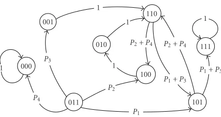
One should immediately notice the difference in defining the reduction and the projection mappings. While the projection is based on the probability distribution of a single gene, the reduction mapping is defined using the probability distribu-tion of the entire collecdistribu-tion of states of the given PBN. To illustrate this difference, we consider one particular example of a PBN (cf. [8]).
Example1. LetA(V,F,C) be a PBN consisting of three genes
V = {x1,x2,x3} and function setsF = (F1,F2,F3), where
F1= {f1(1),f (1)
2 },F2= {f1(2)}, andF3 = {f1(3),f (3)
2 }, and the predictor functions are given by the truth table (Table 1).
Table1
x1x2x3 f(1)
1 f2(1) f1(2) f1(3) f2(3)
000 0 0 0 0 0
001 1 1 1 0 0
010 1 1 1 0 0
011 1 0 0 1 0
100 0 0 1 0 0
101 1 1 1 1 0
110 1 1 0 1 0
111 1 1 1 1 1
c(i)
j 0.6 0.4 1 0.5 0.5
After computing the transition probabilities, (cf. [8]), we arrive at the following directed graph/state transition dia-gram:
1 000
P4 001
P3
011 1
110 1 010
1
100
P2
P1
P2+P4 P2+P4
P1+P3 101
1
111
P1+P3
Here, P1 = 0.3, P2 = 0.3, P3 = 0.2, and P4 = 0.2. Next, we start with a uniform state probability distribution
Din= {1/8, 1/8,. . ., 1/8}for the states in the state spaceSof
A, and then run the corresponding Markov chain for some large number of iterations. Notice that even if the given net-work does not possess a steady state distribution, the re-sult after running the Markov chain sufficiently long time is approximately the stationary state distribution Dthat cor-responds to Din. The simulation gives D = {0.15, 0.0, 0.0, 0.0, 0.0, 0.0, 0.0, 0.85}. Using this distribution, one can com-pute the projected ˆAand the reduced ˜Anetworks, as well as their probability transition matrices. After running the Markov processes associated with these two transition prob-ability matrixes, we obtain the stationary state distributions
ˆ
Dfor ˆA, and ˜Dfor ˜A. For the case when the deleted gene is
x3, we get ˆ
D= {0.006734, 0.022778, 0.138384, 0.831647}, ˜
D= {0.35, 0.0, 0.0, 0.65}. (18)
The stationary state distribution for the transition prob-ability matrix (p∗i,j)4,4i=1,j=1, produced after the collapsing procedure described in part (D) (Section 4), is D1 =
{0.008145, 0.020362, 0.135747, 0.835747}. One can notice the similarity between D1 and ˆD and their apparent dif-ference from ˜D. At the same time, the distribution D∗ = {0.15, 0.0, 0.0, 0.85}described in part (D),Section 4, is simi-lar to ˜D. This should not be surprising—both the projection and the “collapsing” mappings are based on the probability distribution of a single gene, x3 in our example, while the reduction mapping is based on the probability distribution of the entire collection of states in the original PBN. Thus the optimization criterion described inProblem 1becomes a natural compromise between these two possible approaches of reducing the original PBN size.
Inequality (15) can be used in deciding which gene, after being eliminated from the network, will have a minimal im-pact on the stationary distribution of the original PBN. Since the left-hand side of (15) represents the influence In(fj(i)) of a genexnon the predictor fj(i), one can say that, in gen-eral, deleting genes with smaller influences on the remain-ing predictors will result in a better chance of preservremain-ing the stationary state distribution of the original PBN. Here, we provide the values for the influences of x3 on the remain-ing predictors and then two more simulations for the same example, where the other two possible genesx2 andx1 are deleted from the original PBN. The influences of x3on the remaining predictors areI3(f1(1))=0.15,I3(f2(1))=0.15, and
I3(f1(2))=1. After deletingx2fromA, the corresponding sta-tionary state distribution is ˜D= {0.25, 0.0, 0.0, 0.75}, and the influences of x2on the remaining predictors areI2(f1(1)) = 0.15,I2(f2(1))=0.15,I2(f3(1))=0, andI2(f3(2))=0.85. After deletingx1fromA, the corresponding stationary state distri-bution is ˜D= {0.5, 0.0, 0.0, 0.5}, and the influences ofx1on the remaining predictors areI1(f2(1))=1,I1(f3(1))=0, and
It appears that the genex1 with the biggest total influ-ence distorts the stationary state distribution the most but one should be careful when generalizing this observation. Gene influences can be computed based on different prob-ability distributions (cf. [8]). In addition, deleting different genes from the original PBN results in reduced PBNs with different state spaces. Finally, the left-hand side of (15) is just a lower bound that governs the selection procedure in con-structing ˜A, and that the lower bound might not be achieved during the selection procedure.
6. SIMULATION RESULTS
The reduction mapping has been tested using coefficient of determination (COD) microarray data for a networkA con-sisting of 10 genes [23]. The genes of interest in the net-work are PIRIN, WNT5A, S100P, RET-1, MMP-3, PHO-C, STC2, MART-1, HADHB, andSYNUCLEIN. The network is reduced down to 7 genes by subsequently deleting the last three genes, starting withSYNUCLEIN.Table 2presents lists of some of the states in the stationary/steady distributions for the full networkAand the reduced networks ˜A10, ˜A10,9, and ˜A10,9,8, where the indices indicate which genes inAare deleted. For example, ˜A10,9,8 is the reduced network after deleting the genesSYNUCLEIN, HADHB, andMART-1. The states are presented by binary strings of ten digits, where 0 indicates that the corresponding gene is “OFF” and 1 indi-cates that the corresponding gene is “ON.” The leftmost digit representsPIRINand then the remaining digits represent the following genes in the network with the rightmost digit rep-resentingSYNUCLEIN. Next to every given state, its corre-sponding weight in the stationary state distribution of the network is given. Only states with weight bigger than 0.0001 are shown.
One can notice the presence of a very “heavy” state, 1010000111, in the stationary/steady state distribution of the full network. That is in agreement with the COD data set, where the same state is present in 8 out of 31 sam-ples (see [23] for a related discussion). The reduction map-ping maintains the structure of the stationary state distribu-tion of the full network, specifically, the states 101000011, 10100001, and 1010000 carry most of the weight in the sta-tionary/steady state distributions of their corresponding re-duced networks.
7. CONCLUSION
The new mapping introduced in this paper offers a way of re-ducing the size of a given PBN by using the stationary proba-bility distribution on the state space of the PBN. At the same time, it minimizes the distance between the reduced network and the projected PBN introduced in [27]. The distance is given in terms of the distance between their corresponding probability transition matrices. One should notice that the construction of the projected PBN is based on the proba-bility distribution of a single gene, and that the same single gene probability distribution could happen under many dif-ferent stationary distributions on the state space of the orig-inal PBN.
Table2
For the full networkA:
(0000111000, 0.003773); (0000111001, 0.003117); (0001111000, 0.001905); (0010000111, 0.001715); (0100011000, 0.001030); (0100101000, 0.010710); (0100101001, 0.012694); (0100111000, 0.023957); (0100111001, 0.026482); (0101101000, 0.004985); (0101101001, 0.001685); (0101111000, 0.011730); (0101111001, 0.003710); (0110111001, 0.001352); (0111111000, 0.001416); (1010000101, 0.002299); (1010000111, 0.832929)
For ˜A10:
(000011100, 0.010795); (000111100, 0.002513); (001011100, 0.001944); (010010100, 0.140539); (010011100, 0.083694); (010110100, 0.020368); (010111000, 0.001241); (010111100, 0.014547); (011011000, 0.001116); (011011100, 0.005920); (011111000, 0.001743); (011111100, 0.003310); (101000010, 0.001003); (101000011, 0.689413) For ˜A10,9:
(00000110, 0.001528); (00001110, 0.017951); (00011110, 0.004141); (00101110, 0.003209); (01000110, 0.001423); (01001010, 0.230668); (01001100, 0.001481); (01001110, 0.137728); (01011010, 0.033485); (01011100, 0.002186); (01011110, 0.024005); (01101100, 0.001911); (01101110, 0.009774); (01111100, 0.003293); (01111110, 0.005520); (10100001, 0.499967) For ˜A10,9,8:
(0000011, 0.001523); (0000111, 0.020527); (0001110, 0.001065); (0001111, 0.004695); (0010111, 0.003700); (0100011, 0.001814); (0100101, 0.269151); (0100110, 0.001628); (0100111, 0.160629); (0101101, 0.039116); (0101110, 0.002575); (0101111, 0.027858); (0110110, 0.002169); (0110111, 0.011428); (0111110, 0.004034); (0111111, 0.006365); (1010000, 0.429211)
ACKNOWLEDGMENTS
This research was supported by the National Cancer Insti-tute (CA90301), the National Human Genome Research In-stitute, and the Translational Genomics Research Institute.
REFERENCES
[1] L. Glass and S. A. Kauffman, “The logical analysis of con-tinuous, nonlinear biochemical control networks,”Journal of Theoretical Biology, vol. 39, no. 1, pp. 103–129, 1973. [2] S. A. Kauffman, “Metabolic stability and epigenesis in
ran-domly constructed genetic nets,” Journal of Theoretical Biol-ogy, vol. 22, no. 3, pp. 437–467, 1969.
genetic networks: understanding multigenic and pleiotropic regulation,”Complexity, vol. 1, no. 6, pp. 45–63, 1996. [5] Z. Szallasi and S. Liang, “Modeling the normal and neoplastic
cell cycle with “realistic Boolean genetic networks”: their ap-plication for understanding carcinogenesis and assessing ther-apeutic strategies,” inProc. Pacific Symposium on Biocomput-ing (PSB ’98), vol. 3, pp. 66–76, Maui, Hawaii, USA, January 1998.
[6] R. Thomas, D. Thieffry, and M. Kaufman, “Dynamical
be-havior of biological regulatory networks. I. Biological role of feedback loops and practical use of the concept of the loop-characteristic state,”Bulletin of Mathematical Biology, vol. 57, no. 2, pp. 247–276, 1995.
[7] A. Wuensche, “Genomic regulation modeled as a network with basins of attraction,” inProc. Pacific Symposium on Bio-computing (PSB ’98), vol. 3, pp. 89–102, Maui, Hawaii, USA, January 1998.
[8] I. Shmulevich, E. R. Dougherty, S. Kim, and W. Zhang, “Prob-abilistic Boolean networks: a rule-based uncertainty model for gene regulatory networks,” Bioinformatics, vol. 18, no. 2, pp. 261–274, 2002.
[9] I. Shmulevich, E. R. Dougherty, and W. Zhang, “From
Boolean to probabilistic Boolean networks as models of ge-netic regulatory networks,” Proceedings of the IEEE, vol. 90, no. 11, pp. 1778–1792, 2002.
[10] N. Friedman, M. Linial, I. Nachman, and D. Pe’er, “Using Bayesian networks to analyze expression data,” Journal of Computational Biology, vol. 7, no. 3/4, pp. 601–620, 2000. [11] A. J. Hartemink, D. K. Gifford, T. S. Jaakkola, and R. A. Young,
“Using graphical models and genomic expression data to sta-tistically validate models of genetic regulatory networks,” in
Proc. Pacific Symposium on Biocomputing (PSB ’01), pp. 422– 433, Honolulu, Hawaii, USA, January 2001.
[12] E. J. Moler, D. C. Radisky, and I. S. Mian, “Integrating naive Bayes models and external knowledge to examine copper and iron homeostasis in S. cerevisiae,”Physiological Genomics, vol. 4, no. 2, pp. 127–135, 2000.
[13] K. Murphy and I. S. Mian, “Modeling gene expression data using dynamic Bayesian networks,” Tech. Rep., University of California, Berkeley, Calif, USA, 1999.
[14] A. Arkin, J. Ross, and H. H. McAdams, “Stochastic kinetic analysis of developmental pathway bifurcation in phageλ -infected Escherichia coli cells,” Genetics, vol. 149, no. 4, pp. 1633–1648, 1998.
[15] J. Hasty, D. McMillen, F. Isaacs, and J. J. Collins, “Computa-tional studies of gene regulatory networks: in numero molec-ular biology,”Nature Reviews Genetics, vol. 2, no. 4, pp. 268– 279, 2001.
[16] P. Smolen, D. Baxter, and J. Byrne, “Mathematical modeling of gene networks,”Neuron, vol. 26, no. 3, pp. 567–580, 2000. [17] S. Huang, “Gene expression profiling, genetic networks, and
cellular states: an integrating concept for tumorigenesis and drug discovery,”Journal of Molecular Medicine, vol. 77, no. 6, pp. 469–480, 1999.
[18] T. Akutsu, S. Kuhara, O. Maruyama, and S. Miyano, “Iden-tification of gene regulatory networks by strategic gene
dis-ruptions and gene overexpressions,” in Proc. 9th Annual
ACM-SIAM Symposium on Discrete Algorithms (SODA ’98), pp. 695–702, San Francisco, Calif, USA, January 1998. [19] T. Akutsu, S Miyano, and S. Kuhara, “Inferring qualitative
relations in genetic networks and metabolic pathways,” Bioin-formatics, vol. 16, no. 8, pp. 727–734, 2000.
[20] P. D’Haeseleer, S. Liang, and R. Somogyi, “Genetic network inference: from co-expression clustering to reverse engineer-ing,”Bioinformatics, vol. 16, no. 8, pp. 707–726, 2000. [21] S. Liang, S. Fuhrman, and R. Somogyi, “REVEAL, a general
reverse engineering algorithm for inference of genetic
net-work architectures,” inProc. Pacific Symposium on Biocomput-ing (PSB ’98), vol. 3, pp. 18–29, Maui, Hawaii, USA, January 1998.
[22] X. Zhou, X. Wang, and E. R. Dougherty, “Construction
of genomic networks using mutual-information clustering and reversible-jump Markov-Chain-Monte-Carlo predictor design,”Signal Processing, vol. 83, no. 4, pp. 745–761, 2003. [23] S. Kim, H. Li, E. R. Dougherty, et al., “Can Markov chain
models mimic biological regulation?,” Journal of Biological Systems, vol. 10, no. 4, pp. 337–357, 2002.
[24] I. Shmulevich, E. R. Dougherty, and W. Zhang, “Gene pertur-bation and intervention in probabilistic Boolean networks,”
Bioinformatics, vol. 18, no. 10, pp. 1319–1331, 2002.
[25] I. Shmulevich, E. R. Dougherty, and W. Zhang, “Control of stationary behavior in probabilistic Boolean networks by means of structural intervention,” Journal of Biological Sys-tems, vol. 10, no. 4, pp. 431–445, 2002.
[26] A. Datta, A. Choudhary, M. L. Bittner, and E. R. Dougherty, “External control in Markovian genetic regulatory networks,”
Machine Learning, vol. 52, no. 1/2, pp. 169–191, 2003.
[27] E. R. Dougherty and I. Shmulevich, “Mappings between
probabilistic Boolean networks,”Signal Processing, vol. 83, no. 4, pp. 799–809, 2003.
[28] E. R. Dougherty, S. Kim, and Y. Chen, “Coefficient of deter-mination in nonlinear signal processing,” Signal Processing, vol. 80, no. 10, pp. 2219–2235, 2000.
[29] S. Kim, E. R. Dougherty, M. L. Bittner, et al., “General non-linear framework for the analysis of gene interaction via mul-tivariate expression arrays,” Journal of Biomedical Optics, vol. 5, no. 4, pp. 411–424, 2000.
Ivan Ivanovis a Visiting Research Scholar in the Department of Electrical Engineer-ing at Texas A&M University in College Sta-tion and a trainee in the training program in bioinformatics at the Department of Statis-tics at Texas A&M University. He received his M.S. degree in mathematics modeling from Sofia University St. Kilmet Ohridski in 1987 and his Ph.D. degree in mathemat-ics from the University of South Florida in
1999. His current research focuses on genomic signal processing and, in particular, on modeling the genomic regulatory mecha-nisms. He is working in the Genomic Signal Processing Laboratory at Texas A&M University.
Edward R. Dougherty is a Professor in the Department of Electrical Engineering at Texas A&M University in College Station. He holds an M.S. degree in computer sci-ence from Stevens Institute of Technology in 1986 and a Ph.D. degree in mathemat-ics from Rutgers University in 1974. He is the author of eleven books and the editor of other four books. He has published more than one hundred journal papers, is an SPIE