Bivariate genetic association analysis of systolic and diastolic blood pressure by copula models

P R O C E E D I N G S

Open Access

Bivariate genetic association analysis of systolic

and diastolic blood pressure by copula models

Stefan Konigorski

, Yildiz E Yilmaz

, Shelley B Bull

From

Genetic Analysis Workshop 18

Stevenson, WA, USA. 13-17 October 2012

Abstract

We conduct genetic association analysis in the subset of unrelated individuals from the San Antonio Family Studies pedigrees, applying a two-stage approach to take account of the dependence between systolic and diastolic blood pressure (SBP and DBP). In the first stage, we adjust blood pressure for the effects of age, sex, smoking, and use of antihypertensive medication based on a novel modification of censored regression. In the second stage, we model the bivariate distribution of the adjusted SBP and DBP phenotypes by a copula function with interpretable SBP-DBP correlation parameters. This allows us to identify genetic variants associated with each of the adjusted blood pressures, as well as variants that explain the association between the two phenotypes. Within this framework, we define a pleiotropic variant as one that reduces the SBP-DBP correlation. Our results for whole genome sequence variants in the geneULK4on chromosome 3 suggest that inference obtained from a copula model can be more informative than findings from the SBP-specific and DBP-specific univariate models alone.

Background

A number of genome-wide association studies (GWAS) involving large populations have been conducted to iden-tify genetic variants associated with various single blood pressure (BP) measures: systolic blood pressure (SBP), diastolic blood pressure (DBP), or a linear function of them. Although the correlation between SBP and DBP is high, the results of the GWAS for each separately indi-cate only partially overlapping sets of variants associated with SBP and DBP. In this report, we model SBP and DBP jointly, taking the association between them into account. Constructing a bivariate model for these two phenotypes can increase the power to detect causal var-iants for one or both phenotypes, shedding more light onto the complex underlying genetic processes.

We apply copula functions [1] to model the bivariate distribution of SBP and DBP conditional on genetic var-iants. Copulas are functions used to construct a joint distribution by combining the marginal distributions

with a dependence structure, and they allow investiga-tion of the dependence structure between the pheno-types SBP and DBP separately from the marginal distributions. This property of copula models is very useful in identifying genetic variants that explain the dependence between SBP and DBP. It is well known that the Pearson correlation coefficient effectively mea-sures the linear dependence of two random variables coming from a bivariate normal distribution. However, it may not be a good measure for other bivariate distri-butions where the conditional mean ofYigivenYjis not

linear inYj. Hence, we prefer a nonparametric correla-tion measure. One frequently used measure based on concordance and discordance is Kendall’s tau, which is the probability of concordance minus the probability of discordance. We also use upper and lower tail depen-dence measures, which measure the level of dependepen-dence in the upper-right quadrant tail and lower-left quadrant tail of a bivariate distribution, respectively, as it might be especially interesting to find pleiotropic variants explaining association between high SBP and high DBP or low SBP and low DBP.

Our analysis has two objectives: (a) to investigate the association of some common variants with SBP and DBP

* Correspondence: yyilmaz@mun.ca

†Contributed equally

1

Dalla Lana School of Public Health, University of Toronto, 155 College Street, Toronto, ON, M5T 3M7, Canada

Full list of author information is available at the end of the article

under the joint model of SBP and DBP, and (b) to iden-tify pleiotropic variants, which we define as variants that explain the association between SBP and DBP.

Methods

San Antonio family studies data

The Genetic Analysis Workshop 18 (GAW18) data set includes 153 unrelated individuals from the San Antonio family studies pedigrees having SBP and DBP measure-ments at one or more study exams, information regarding current use of antihypertensive medication, and nonge-netic covariates sex, age, and current tobacco smoking status at some examinations. To retain all subjects, we imputed missing age values by adding the mean time interval between measurements to the last known age of a subject. Some missing values of smoking status were also imputed by examining the smoking patterns of individuals over the four time points. We later verified that these imputations did not lead to any significant differences in parameter estimates and inference. Among the 153 unre-lated individuals with measured phenotype data, 100 have whole genome sequence data. We conducted our genetic analysis on chromosome 3 in this group, considering only theULK4gene previously found to be associated with DBP [2]. We analyzed 1771 variants with minor allele frequency (MAF)≥0.05.

Phenotype definition

Before modeling the joint distribution of SBP and DBP conditional on genetic variants, we first adjusted the observed BPs for the effect of antihypertensive medication and other nongenetic covariates. The GAW18 unrelated pedigree members include hypertensive individuals (i.e, with high BP) and some taking antihypertensive medica-tion (Table 1). Adjusting BP for the effect of BP-lowering medication is crucial when the objective is to identify genes associated with high or low BP. Based on a simula-tion study comparing several methods [3], the use of a censored regression model conditional on both nongenetic and genetic covariates was recommended, assuming that a treated individual’s true“underlying” BP is higher than

that observed. For our analysis, we extend their censored regression approach by deriving the maximum likelihood estimate (MLE) of a conditional expectation that is in the form of fitted BP plus a nonnegative adjustment term depending on the observed BP and the nongenetic covari-ates. It provides a more intuitive adjustment of the BP of treated individuals than, for example, the nonparametric method or assuming that treatment has the same constant effect for each individual as in Tobin et al [3].

At each examination point j j, we separately fitted censored regression models of BP conditional on nonge-netic covariates age, sex, and smoking status with medi-cation use as the censoring indicator. After conducting standard residual analysis and model selection, we speci-fied the models as

formulation of the age covariates reflects previous findings (see, eg, Ref. [4]) that SBP increases with age whereas DBP decreases after the age of 55 to 60 years, which can be approximated here with the sample mean age. We used the“survreg”function in the“survival”package of R to fit the censored regression models.

For individuals who received antihypertensive medica-tion, we estimate the underlying BP with the MLE of the conditional expectation of BP, given that the observed BP is lower than the true underlying BP. For illustration, under the model (1), the conditional expec-tation is

wherezi,jdenotes the vector of nongenetic covariates with associated regression parameterγ(j)=

γ0(j),γ1(j),γ2(j),γ3(j)

,

and f,Fare the normal probability density and cumulative distribution functions, respectively, with meanγ(j)zi,jand

variance σSBP,j2. The effects of the adjustment are

evi-dent in Figure 1, with the adjusted BP of treated indi-viduals always higher than their observed BP. At each of the first 3 examination time points, we obtained residuals from fitting the censored regression models (1) and (2). We disregarded the last examination time because few BP measurements were available (see Table 1). An untreated individual’s residual is the dif-ference between observed and fitted BPs; a treated individual’s residual is the difference between adjusted and fitted BP. Finally, we averaged the residuals (over j = 1,2,3) separately for SBP and DBP, and took these mean residuals as our adjusted phenotypes.

Table 1 Number of unrelated individuals, hypertensive individuals, and individuals on antihypertensive medication

Exam 1 Exam 2 Exam 3 Exam 4

Total* 141 97 98 37

Hypertensive† 42 49 52 27

Receiving meds 27 30 45 25

*Number of unrelated individuals having SBP and DBP measurements and current use of antihypertensive medication available at the examination time point used in the phenotype adjustment.

Bivariate copula modeling

In the second stage, we first constructed the marginal models for our adjusted phenotypes Y1andY2given a

genetic variant X=x, assuming that the genetic variants

Xare independent of the nongenetic variants Z. In the marginal models

Y1,i=α0+α1xi+iandY2,i=β0+β1xi+i (4)

we observed no evidence against the normality assumptions for the error terms. We then used a copula functionCto build the bivariate distribution ofY1and Y2conditional on genetic variants by combining the 2

marginal distribution functions F1

y1|X=x

and

F2

y2|X=x

. More specifically, we consider the bivariate distribution function

Fy1,y2|X=x

=C_ψF1

y1|X=x

,F2

y2|X=x

(5)

where F1and F2are the normal cumulative

distribu-tion funcdistribu-tions with variances_σ12_andσ

22, respectively,

andψis the vector of copula parameters. To illustrate the approach, consider the 2-parameter copula family

Cψ(u1,u2)=u1−ϕ−1

θ

+u2−ϕ−1

θ 1/θ + 1

₋1/ϕ

(6)

with0≤u1,u2≤1,and the copula (or dependence)

parameters ψ=(ϕ,θ),ϕ >0,θ ≥1. To explain the association betweenY1andY2, we use Kendall’s tau(τ),

which is a measure of overall association based on con-cordance and discon-cordance, and we use lower and upper tail dependence measures (lL, lU, respectively), which

explain the amount of dependence between extreme values, and can give more insight in identifying pleiotro-pic variants. For the copula family in (6), these depen-dence measures become [1]

τ = 1− 2

θ (ϕ+ 2),λL= 2 −1/θϕ_,λ

U= 2−2−1/θ (7)

We obtain MLEs of the marginal parameters β=(β0,β1,σ2), β=(β0,β1,σ2)in equation (4) and the

copula parametersψ=(ϕ,θ)in equation (6) by maxi-mizing the likelihood function [1] with the general opti-mization software implemented in the nlm function in R. Variance estimates for the MLEs are obtained from the inverse of the observed information matrix.

To address aim (a) concerning the marginal association of a variant with each SBP and DBP under the bivariate model (5), we test the null hypothesesH0:α1= 0(vs. HA:α1= 0) and H0:β1= 0 (vs. HA:β1= 0) with the

large sample Wald test statistic. We expect improved inference under the bivariate model compared to inference obtained by separate analysis of SBP and DBP, which we refer to as the working independence model.

In contrast, for aim (b), which is to identify a variant that explains association between SBP and DBP, the copula model dependence parameters ϕ and θ, and dependence measures (7) are of interest. We compare estimates of Kendall’sτ,λL, andλUunder the full

bivari-ate model (5) that includes the genetic variant with the corresponding estimates obtained under the bivariate model without the variant (ie, the null model with

H0:α1=β1= 0). According to the delta method, we

construct a confidence interval (CI) for the dependence measures using large-sample standard errors. When the CIs for a given association measure under the null and the full model do not overlap, we conclude that the given variant is pleiotropic. Use of CIs in this way is quite con-servative. We also check whether the CI forλLorλU

under the full model includes 0. Note that the copula model (6) only becomes an independent copula

C(u1,u2) =u1u2whenθ = 1andϕgoes to 0. However,

because it is practically impossible to identify all variants, instead of testing independence, we search for variants that reduce the magnitude of the overall dependence measures, such as Kendall’sτ.

Results and discussion

For model selection, we note that the Akaike informa-tion criterion (AIC) value under the copula model (6) is much lower than the AIC under a bivariate normal model, indicating that the copula model is a better fit. For example, the AIC value under the copula model (6) reported in Table 2 is 1227.6 compared to an AIC value of 1337.8 under the bivariate normal model (not shown). These AICs are comparable to those obtained when conditioning on other variants. The aim (a) results (Table 2) are thus limited to the Wald testp values of the MLE estimates of the coefficientsα1, β1in (4) for

testing H0:α1= 0andH0:β1= 0under two models:

the working independence model and the bivariate copula model (6) for single-variant analysis. We observed some variants, including less common (0.05 ≤ MAF ≤0.10) and more common (MAF >0.10) variants, that are identified by both models, but the pvalues for testing H0:α1= 0 and H0:β1= 0 under the copula

model (with minimumpvalues 1.7 × 10−4and 5.1 × 10

−5

, respectively) are smaller than thepvalues under the working independence model (with minimumpvalues 5.5 × 10−3 and 7.0 × 10−4, respectively). This includes variants significantly associated with both BP pheno-types under the joint copula model, although they are not significantly associated at the 1% level with either under the univariate phenotypic models (see Table 2). Overall, the estimated genetic effect sizes are larger and the estimated standard errors are slightly smaller under the bivariate model.

Table 3 displays 2 of 10 variants yielding a substantial reduction in point estimates of the upper tail dependence

measureλUunder the bivariate model (5) conditional on

the variant. Compared to the null model when condition-ing on a variant in the geneULK4, Kendall’s tau and lower tail dependence do not differ markedly. We observe that without conditioning on any variant (H0:α1=β1= 0), the 2 phenotypes are moderately

cor-related with a Kendall’s tau estimate of 0.578, and higher lower tail dependence than upper tail dependence (Table 3). Conditioning on the variant at 41,984,243 base-pair position diminishes upper tail dependence measureλUat

0.01 level of significance (99% CI forλUincludes 0); this

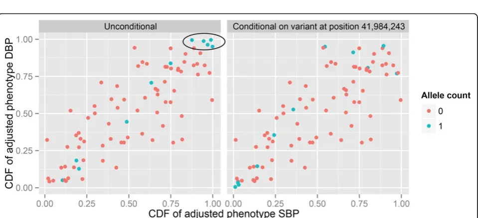
variant is also associated with SBP and DBP (see Table 2). Figure 2 illustrates how it achieves a reduction in upper tail dependence. Tail dependence can also be reduced in the absence of strong marginal BP associa-tions. For example, the variant at 41,971,559 base-pair position is only modestly associated with SBP (pvalue = 0.040) and DBP (pvalue = 0.055), but the upper tail dependence is reduced from 0.449 obtained under the null model to 0.289 with a CI that includes 0 (Table 3).

Conclusions

In this report, we demonstrate how to model the bivari-ate distribution of SBP and DBP with copulas and con-duct appropriate inference for genetic association. The proposed method is shown to be applicable by consider-ing a sconsider-ingle gene, and crude estimates of computation time suggest that it is feasible to process 1 million var-iants in less than a day, for example, by using one hun-dred 2.5-GHz cores. Although estimating the bivariate distribution is computationally more intensive than fit-ting the working independence model, given the high correlation between the phenotypes, a potential advan-tage is that genetic associations can be detected with higher power under a plausible joint model. Using joint copula models, we were also able to identify candidate variants explaining the upper tail dependence of SBP and DBP. We generally observed strong linkage disequili-brium between variants identified. By conducting joint analyses of multiple variants in moderate linkage disequi-librium, we achieved a much more significant reduction in upper tail dependence (data not shown), and although we observed some reduction in point estimates of lower tail dependence and Kendall’s tau, the CIs still overlap with those under the null model. Calling a comparison significant when the CIs fail to overlap is a conservative

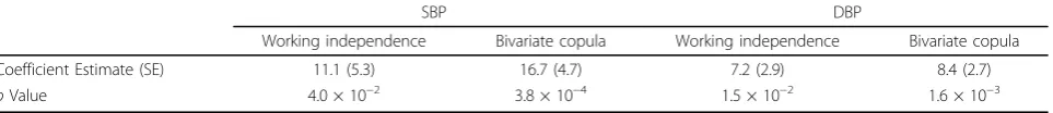
Table 2 Results of testingH0(α) :α1= 0orH0(β):β1= 0for variant at 41,984,243 base-pair position

SBP DBP

Working independence Bivariate copula Working independence Bivariate copula

Coefficient Estimate (SE) 11.1 (5.3) 16.7 (4.7) 7.2 (2.9) 8.4 (2.7)

pValue 4.0 × 10−2 _{3.8 × 10}−4 _{1.5 × 10}−2 _{1.6 × 10}−3

approach, but it is computationally efficient. As an alter-native, a nonparametric bootstrap procedure could be used to estimate the variance of the estimated difference between dependence measures under the null and full models, and to construct an approximate CI. To allow mul-tiple testing adjustments, instead of checking whether the CI forλLorλUunder the full model includes 0, it would be

desirable to test each of the null hypothesesH0:ϕ= 0or H0:θ = 1, respectively, to obtainpvalues [5].

In principle, the extension of our approach to 3 or more quantitative traits is straightforward; however, the copula model (6) may not be ideal in this setting. It involves some restrictions on the association structure, and generally the Gaussian copula is used when there are 3 or more traits. The approach could also be extended to binary traits, but with some caution because there is no unique copula identifying the joint distribu-tion funcdistribu-tion of discrete variables [6].

Competing interests

The authors declare that they have no competing interests.

Authors’contributions

YEY and SBB designed the overall study, SK conducted statistical analyses, and SK and YEY drafted the manuscript. All authors read and approved the final manuscript.

Acknowledgements

YEY was supported by a MITACS Network Industrial Fellowship, the Syd Cooper Fund and is a CIHR Fellow in Genetic Epidemiology and Statistical Genetics with CIHR STAGE (Strategic Training for Advanced Genetic Epidemiology). This work was supported in part by grants from the MITACS Network of Centres of Excellence in Mathematical Sciences and the Natural Sciences and Engineering Research Council of Canada. The GAW18 whole genome sequence data were provided by the T2D-GENES Consortium, which is supported by NIH grants U01 DK085524, U01 DK085584, U01 DK085501, U01 DK085526, and U01 DK085545. The other genetic and phenotypic data for GAW18 were provided by the San Antonio Family Heart Study and San Antonio Family Diabetes/Gallbladder Study, which are supported by NIH grants P01 HL045222, R01 DK047482, and R01 DK053889. The Genetic Analysis Workshop is supported by NIH grant R01 GM031575. This article has been published as part ofBMC ProceedingsVolume 8 Supplement 1, 2014: Genetic Analysis Workshop 18. The full contents of the supplement are available online at http://www.biomedcentral.com/bmcproc/ supplements/8/S1. Publication charges for this supplement were funded by the Texas Biomedical Research Institute.

Authors’details 1

Dalla Lana School of Public Health, University of Toronto, 155 College Street, Toronto, ON, M5T 3M7, Canada.2_{Current address: Molecular}

Table 3 Estimates of dependence measures(τ,λL,λu)under the null modelH0:α1=β1= 0and under model (5) in a single-variant analysis

Variant τ (SE) (99% CI forτ) _λL(SE) (99% CI forλ_L) _λU(SE) (99% CI forλ_u)

Null 0.578 (0.05) (0.449, 0.707) 0.650 (0.07) (0.470, 0.830) 0.449 (0.10) (0.191, 0.707) 41,984,243 0.555 (0.06) (0.400, 0.710) 0.703 (0.06) (0.548, 0.858) 0.268 (0.21) (0.000, 0.809) 41,971,559 0.570 (0.05) (0.441, 0.699) 0.715 (0.06) (0.560, 0.870) 0.289 (0.18) (0.000, 0.753)

Figure 2Scatterplots of the cumulative distribution function ofY1(F1)versusY2(F2)without conditioning on any variant (left panel) and conditional on the variant at 41,984,243 base-pair position (right panel). The indicated blue dots denote individuals with high adjusted

Epidemiology Group, Max Delbrück Center for Molecular Medicine (MDC), Robert-Rössle-Straße 10, 13125 Berlin, Germany.3_{Lunenfeld-Tanenbaum}

Research Institute of Mount Sinai Hospital, 60 Murray Street, Box 18, Toronto, ON, M5T 3L9, Canada.4_{Current address: Department of Mathematics and}

Statistics, Memorial University of Newfoundland, St. John’s, NL, A1C 5S7, Canada.

Published: 17 June 2014

References

1. Joe H:Multivariate Models and Multivariate Dependence Concepts.

London, Chapman & Hall1997.

2. Ehret GB, Munroe PB, Rice KM, Bochud M, Johnson AD, Chasman DI, Smith AV, Tobin MD, Verwoert GC, Hwang S,et al:Genetic variants in novel pathways influence blood pressure and cardiovascular disease risk.Nature2011,478:103-109.

3. Tobin MD, Sheehan NA, Scurrah KJ, Burton PR:Adjusting for treatment effects in studies of quantitative traits: antihypertensive therapy and systolic blood pressure.Stat Med2005,24:2911-2935.

4. Sesso HD, Stampfer MJ, Rosner B, Hennekens CH, Gaziano JM, Manson JE, Glynn RJ:Systolic and diastolic blood pressure, pulse pressure, and mean arterial pressure as predictors of cardiovascular disease risk in men.

Hypertension2000,36:801-807.

5. Yilmaz YE, Lawless JF:Likelihood ratio procedures and tests of fit in parametric and semiparametric copula models with censored data.

Lifetime Data Anal2011,17:386-408.

6. Genest C, Neslehova J:A primer on copulas for count data.ASTIN Bull

2007,37:475-515.

doi:10.1186/1753-6561-8-S1-S72

Cite this article as:Konigorskiet al.:Bivariate genetic association analysis of systolic and diastolic blood pressure by copula models.BMC Proceedings20148(Suppl 1):S72.

Submit your next manuscript to BioMed Central and take full advantage of:

• Convenient online submission

• Thorough peer review

• No space constraints or color figure charges

• Immediate publication on acceptance

• Inclusion in PubMed, CAS, Scopus and Google Scholar

• Research which is freely available for redistribution