UWB pulse detection and TOA estimation using GLRT

(1)

R E S E A R C H

Open Access

UWB pulse detection and TOA estimation

using GLRT

Yan Xie

1*

, Gerard J.M. Janssen

1

, Siavash Shakeri

2

and Christiaan C.J.M. Tiberius

2

Abstract

In this paper, a novel statistical approach is presented for time-of-arrival (TOA) estimation based on first path (FP) pulse detection using a sub-Nyquist sampling ultra-wide band (UWB) receiver. The TOA measurement accuracy, which cannot be improved by averaging of the received signal, can be enhanced by the statistical processing of a number of TOA measurements. The TOA statistics are modeled and analyzed for a UWB receiver using threshold crossing detection of a pulse signal with noise. The detection and estimation scheme based on the Generalized Likelihood Ratio Test (GLRT) detector, which captures the full statistical information of the measurement data, is shown to achieve accurate TOA estimation and allows for a trade-off between the threshold level, the noise level, the amplitude and the arrival time of the first path pulse, and the accuracy of the obtained final TOA.

Keywords: Ultra-wide band (UWB), Time-of-arrival (TOA) estimation, Sub-Nyquist sampling, GLRT, Ranging, Positioning

1 Introduction

The demand for accurate wireless positioning in indoor environments is vastly increasing for precise localization and tracking of objects and people, with applications in a.o. industry, warehouses, shopping malls, and hospitals. In these environments, traditional positioning solutions based on satellite signals are unreliable, unavailable, or do not provide sufficient accuracy. In recent years, much attention has been given to ultra-wideband (UWB) sig-nals for indoor positioning. UWB sigsig-nals, e.g., sub-nano-second duration pulse signals, enable precise ranging because they allow for separation of multipath components and accurate estimation of the time-of-arrival (TOA) of the first arriving path (FP) signal [1, 2]. With this feature of UWB signals, centimeter-level ranging accuracy can be achieved, even in dense multipath environments [2, 3].

In recent decades, researchers have been developing several approaches to get the TOA of the received FP pulse. In [3, 4], pulses with sub-nanosecond duration are transmitted and then measured with a digital sam-pling scope with full samsam-pling rate as the receiver. Based on the recovered received signal, time-domain TOA

*Correspondence: [email protected]

1_{Faculty of Electrical Engineering, Mathematics and Computer Science, Delft}

University of Technology, Mekelweg 4, 2628 CD Delft, The Netherlands Full list of author information is available at the end of the article

estimation algorithms, which are typically maximum like-lihood (ML)-based approaches [5–7], are applied by iden-tifying the FP from the sampled signal. Besides, [8–13] get the received pulses by setting up a frequency domain measurement system using a vector network analyzer (VNA) to record the frequency response of the channel. This measured frequency response can be converted to the time domain by taking the inversed Fourier trans-form, or a variety of super-resolution techniques, such as root multiple signal classification (MUSIC) [14] and total least square-estimation of signal parameter via rotational invariance (TLS-ESPRIT) [15], can be applied to increase time-domain resolution based on frequency response measurements. On the other side, the wide bandwidth of UWB signals, usually in the gigahertz (GHz) range, puts high demands on the sampling circuit to satisfy Nyquist sampling rates, which are easily several Giga-samples per second (GS/s). In order to overcome this disadvantage, researchers resort to sub-Nyquist sampling techniques for ranging using sub-nanosecond pulse signals. In [16, 17], compressed sampling techniques are applied to realize sub-Nyquist sampling at the expense of a more complex receiver structure. Fontana and Gunderson [18] gives a novel design to obtain TOA measurements directly with-out sampling of the received signal, where a receiver is used based on a daisy-chain structured tunnel diode

(2)

detector to detect successive peaks of the measured chan-nel impulse response. The benefit of this method is that, TOA measurements are obtained directly without the use of high-sampling rate circuits or universal test instru-ments, which allows the receiver to be highly integrated, of low complexity and low cost. However, compared with Nyquist sampling-based and compressive sampling-based TOA estimation schemes, TOA estimation schemes based on direct TOA measurements have not been investigated in-depth in the literature.

In the following, we further investigate the idea of direct TOA measurements, where the time instant at which the received signal crosses a preset threshold voltage is detected using a sub-Nyquist sampling technique. This threshold voltage is chosen such that the probability of threshold level crossing is due to noise only and the probability of false alarm, PFA, is at an acceptable low

level. Therefore, the first threshold-exceeding signal in each measurement period of the receiver can be consid-ered caused by the transmitted pulse signal traveling via the shortest path, and the measured TOA of this sig-nal is recorded. However, a measurement event might be wrongly recorded as a TOA when the threshold level was crossed due to noise before arrival of the pulse, or the pulse might be miss-detected due to its low power level compared to the threshold and a late path signal may be detected. Thus, the threshold value, which should be set based on both the noise level and the expected pulse level, determines the probability of correct pulse detection as well as the sensitivity of the receiver.

The analysis of threshold selection has not been addressed in detail in early researches. In [1], an approach is given on the kurtosis of the signal samples for threshold selection by applying an energy detector to capture both the statistics of the channel and the SNR of the received signal. However, this TOA estimation method is based on full Nyquist sampling of the received signal and TOA estimation accuracy is at meter level.

Receiver and detection techniques which operate at a much lower sample rate than Nyquist were proposed in [2, 19] and [20]. In this detector, the crossing of a preset threshold level triggers the discharging of an RC circuit with an accurately known RC-time and therefore discharge curve. With only a few samples of this curve, the precise start of the discharging process can be esti-mated. Triggering of the discharging process can happen due to a received signal pulse but also (occasionally) due to noise. However, noise may also cause a deviation of the trigger moment from the actual arrival instant of the pulse. Since it is not feasible to apply signal averag-ing to improve the probability of detection (PD) of this

sub-Nyquist-based receiver structure, we need to resort to another approaches to maximize PD. In [2] and [3],

TOA estimation performance is statistically analyzed for

the threshold level selected based on the pre-set PFA.

The technique for estimating the TOA proposed in [2] is based on finding a sliding time-window which contains at least a certain predetermined minimum number of TOA events, which depends on channel quality (SNR, SIR) and the number of measured events. The mean TOA of the events within the sliding window was selected as the esti-mated TOA. A disadvantage of this technique is that a large time window following the arming of the detector had to be excluded from TOA estimation because of the high number of level crossings due to noise only in that range, and therefore making the detector less efficient. The results in [2] show that a higher estimation accu-racy can be achieved compared to energy-based detection schemes; however, since the distribution of the measured TOA events due to noise and the preset detector threshold is not exploited, there is room for improvement of both the TOA estimation accuracy and the receiver’s sensitivity. In this paper, an improved TOA estimation method is proposed which takes into account the distribution of the measured TOA events: the time distribution of the mea-sured first level-crossing events due to noise only, which strongly depends on the time-duration since arming the detector, and the distribution of the first level-crossing events in case a pulse plus noise was received. The pulse detection and TOA estimation are based on the GLRT detector, using the likelihood ratio of the TOA distribu-tion. By exploiting the full statistical information of the measurement data, receiver sensitivity and the accuracy of the estimated TOA can be substantially improved.

This paper is organized as follows. In Section 2, the signal model and the low-complexity TOA sub-Nyquist sampling receiver structure are described. In Section 3, a mathematical model of the first threshold crossing is derived for this receiver which is subsequently used to obtain the probability density function (PDF) of the mea-sured TOA events. The noise variance as well as the FP pulse amplitude can be estimated based on this PDF and the recorded statistics of the measured TOA events. Moreover, the relation among threshold-level, noise vari-ance, and the FP pulse amplitude is analyzed. In Section 4, the TOA is estimated using composite hypothesis test-ing based on the joint PDFs of the TOA measurements. Simulations show that the GLRT results in a vast improve-ment of the TOA estimation performance. Conclusions are drawn in Section 5.

2 System model

2.1 Signal model

The transmitted signal is composed of a sequence of pulses, which can be written as a function of timet:

s(t)=

∞

k=−∞

(3)

wherew(t)is the waveform of a single pulse,Tf is the

rep-etition period of the transmitted pulses, andkis the index of a specific time frame.

Accordingly, the received signal in a static multipath channel can be represented as:

r(t)=

∞

k=−∞ L−1

l=0

hlw(t−tl−kTf)+n(t), (2)

where hl and tl are the amplitude and delay of the l-th

multipath component, respectively, andLis the number of multipath components, andn(t)is zero-mean additive white Gaussian noise with power spectral density (PSD)

σ2

0. For the purpose of ranging, the means for multiple access are not considered in this signal model.

2.2 Receiver model

The analysis in this paper is based on a low-complexity receiver structure for UWB TOA measurements, which is a slightly adapted version of the receiver proposed in [2, 19, 20]. Instead of applying full Nyquist sampling on the received signal, this receiver detects the signal which first crosses a pre-set threshold voltage in each measurement period and records the arrival time of this signal, which is assumed to be the FP signal, with respect to the start of the measurement period. For simplicity, the measurement period is taken equal to the pulse repetition periodTf.

Figure 1 shows the block diagram of the proposed receiver. After amplification and band-pass filtering (BPF) of the signal r(t) received by the antenna, the signal v(t) is compared with a pre-set threshold levelVNin a fast

com-parator. The periodic measurement window is started by the local clock. Whenv(t) > VN for the first time after

the start of a measurement window, the rising edge of the comparator outputVCMP latchesVSP. The latched signal VSP triggers the TOA measurement process and blocks

the next threshold crossings, e.g., due to multipath sig-nals, during the remainder of the measurement period. The time-measurement unit determined the TOA of the FP with respect to the start of the current measurement window using the time estimation presented in [19, 20]. We denote the FP’s TOA measurement in thek-th repeti-tion period astM[k] and we collectKTOA measurements

inKsuccessive measurement windows.

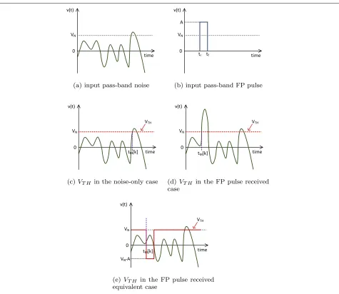
The input signalv(t)of the comparator in Fig. 1 includes the BPF filtered noise shown in Fig. 2a, and the fil-tered multi-path pulse signal. To simplify the analysis, we assume that the BPF is an ideal filter with a lower cut-off frequency offL and an upper cutoff frequency offH,

respectively, and the pulses inv(t)to be rectangular with durationtw. Figure 2b shows the FP pulse with amplitude A(A> 0 when it is a positive pulse, orA< 0 for a neg-ative pulse), rising edge attr, and falling edge attf, where tf −tr = tw. In the noise-only case (A = 0), the

thresh-old voltageVTHof the system is equal to the pre-set level VTH =VN of the comparator, as shown in Fig. 2c. When

the FP pulse is received (A > 0 or A < 0), the input signalv(t), which includes both pulse and noise, is com-pared toVTH = VN, as shown in Fig. 2d. However, this

case can also be considered as a special noise-only case where the thresholdVTHis changed to(VN −A)during

the time interval [tr,tf] and stays atVNfor the rest of time,

as illustrated in Fig. 2e. In this way, pulse detection can be modeled in a unified way as a first-threshold-crossing problem of filtered noise only, with

VTH=

VN−A, tr≤tM[k]≤tf

VN, otherwise . (3)

From a large number of measured pulse arrival times, the probability density function (PDF) of a single pulse measurement and the joint PDFs of allKcollected pulse measurements under two different conditions: noise-only case and pulse received case, can be obtained for this first-threshold-crossing model. These two PDFs can be used in a composite hypothesis test for estimating the FP’s TOA. Processing of the TOA measurementstM[k]|k=1,···,K to

estimate its true TOA is the topic of Section 3.

3 TOA estimation

3.1 First-threshold-crossing problem

Consider the noise-only case, where, after bandpass fil-tering as shown in Fig. 1, the voltagev(t)has a PSD of

Pvv(f) = σ₀2 forfL < |f| < fH andPvv(f) = 0

out-side this pass-band. Now, we find the probability ofv(t) < VTHin the time interval(0,t), whenv(t)first crosses the

levelVTHin the time interval(t,t+dt). This problem is

called the first-crossing problem [21, 22]. The PDF of the

(4)

Fig. 2Equivalence of the signal level-crossing model:athe input signal only containing band-pass (BP) noise,bthe input signal only containing an FP pulse,ca threshold crossing due to BP noise only withVN=VTH,dA threshold crossing when the input is the summation of BP noise and an FP

pulse withVN=VTH,eis the equivalent model of (d), where the input signal contains only BP noise whileVTHchanges toVN−Aduring an FP pulse

arrival

first-crossing byv(t)at timet,pc(VTH,t), is an exponential

distribution given by

pc(VTH,t)=μ[VTH,t|(0,t)]e−μ[VTH,t|(0,t)]t (t>0),

(4)

where μ[VTH,t|(0,t)] is the probability of an upward

crossing in (t,t+ dt) with no prior upward crossing in

(0,t), [22].

Specifically, considering the statistically rare crossings of a high-level VTH, [21, 23, 24] suggest the following

approximation to (4):

pc(VTH,t)NTH+ e−N +

THt (_t>₀)_, ₍₅₎

whereN_TH+ is the expected number of upward crossings of v(t)=VTHper unit of time.

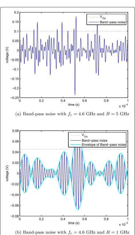
In the noise-only case, v(t) can be approximated as white noise when the filter bandwidthB= fH−fLis

rel-atively large compared to its center frequencyfc= fH+₂fL,

as shown in Fig. 3a. In this case,v(t)andv˙(t)= dv_dt(t)can be considered as statistically independent, thusN_TH+ can be obtained from

N_TH+ = _∞

0 ˙

vp(v,v˙;t)dv˙ v(t)=VTH

, (6)

(5)

Fig. 3Bandpass noise waveforms:aa waveform of BP noise with relatively largeB/fcwhich corresponds to the case of (17),ba

waveform of BP noise with relatively smallB/fcwhich matches the

case of (18)

tv˙ =v/˙v, p(v,v˙;t)_t_v_˙vv˙

v(t)=VTH

= ˙vp(v,˙v;t)v˙_v₍_t₎₌_V TH indicates the expected number of positive passages ofv(t) per unit time through the interval [VTH,VTH+v] for a

given value ofv˙, wherev→0 andv˙→0.

When B is small compared tofc, v(t) has the typical

characteristics of a band-pass signal of which the enve-lope changes are proportional toB−1, as shown in Fig. 3b. Accordingly,v(t)can be expressed as a random envelop modulating a sinewave carrier signal with frequencyfcand

a random phase angleθ(t), given by

v(t)=c(t)cos2πfct+θ(t)

, (7)

wherec(t) is the Rayleigh distributed envelope and θ(t) the uniformly distributed phase ofv(t).

From Fig. 3b and (7) we find that the threshold up-crossings ofv(t)come in clusters and they can only occur after c(t) has an up-crossing event. Therefore, the first upward threshold-crossing of v(t) occurs after the first up-crossing ofc(t). The actual signal crossing will have a uniformly distributed time delay in the range of0, 1/fc

with respect to the envelope up-crossing. In this case, the PDF of the first-threshold-crossing probability of the envelop c(t) can be considered as the first-threshold-crossing probability of the band-pass noisev(t), where the actual detection moment shows an extra delay of on aver-age 0, 1/2fc . As a result, the rate of upward crossings N_TH+ in this case is

N_TH+ = ∞

0 ˙

cp(c,˙c;t)dc˙ c(t)=VTH

, (8)

wherec(t)andc˙(t)are independent,˙c(t)has a Gaussian distribution andp(c,˙c;t)is the joint PDF forc(t)and˙c(t). In order to obtain all the parameters in the joint PDF ofp(v,v˙;t)andp(c,c˙;t), we need to calculate the variance ofv(t),˙v(t),c(t), andc˙(t), respectively. According to the Wiener-Khinchine relations,

Rvv(τ)=

_∞

−∞Pvv(f)e

j2πfτ_df _,

R˙v˙v(τ)=

_∞

−∞P˙v˙v(f)e

j2πfτ_df _,

(9)

whereRvvandRv˙v˙are the autocorrelation functions of the

random processesv(t) andv˙(t), respectively.Pvv(f) and

Pv˙v(˙ f)are the PSD ofv(t)andv˙(t), respectively, and they

have the relationP˙v˙v(f) = (2πf)2Pvv(f). Therefore, we

obtain the relation that

Rvv(τ)= ∞

−∞

j2πf2Pvv(f)ej2πfτdf

= −Rv˙v(τ)˙ ,

(10)

whereindicates the second derivative operator.

Letψ0=Rvv(τ)|τ=0andψ1=R˙cc(τ)˙ |τ=0, which are the variances ofv(t)and˙c(t), respectively. Then, from (10), we haveψ₀ = −Rv_˙v(τ)˙ |τ=0, and from (7), we can getψ0 = Rcc(τ)|_τ₌0. Moreover, we determineψ1by expanding the derivative of (7) as

˙

v(t)=˙c(t)cos2πfct+θ(t)

−

c(t)2πfc+ ˙θ(t) sin

2πfct+θ(t) ,

(11)

where (11) is a linear combination of two independent random processes, and its variance is the sum of the two variances and reduces to

(6)

In the receiver of Fig. 1, the input signal as well as the noise is filtered by an ideal band-pass filter. For band-limit noise,

, then we find for the up-crossing rateN_TH+ for largeB/fc

(17) and (18) are equal. We can use (19) as the division of relatively “narrow-band” case and “wide-band” case.

Now (5), (17), and (18) reveal thatN_TH+ and the PDF of the first-crossing timepc(VTH,t) can be computed from

the pre-set parameters VTH, fH, fL, and the PSD of the

noise σ₀2. Moreover, the PDF of a single TOA ment and the joint PDF of a number of TOA measure-ments can be obtained based onpc(VTH,t), which will be

further discussed in Sections 3.2 and 3.3. However, when

σ0is unknown, it can be estimated from the empirical PDF of the first-crossing time which can be obtained from a set of TOA measurements, as will be shown in Sections 3.2 and 3.3.

3.2 PDF of a single TOA measurement

Consider the PDF of the k-th pulse arrival time mea-surement, recorded as tM[k]. In the noise-only case, as

indicated in (5), this PDF is

p(tM[k] ;μ1)=μ1e−μ1tM[k] tM[k]>0 , (20)

andμ2is the coefficient of the PDF for the pulse duration whereVTH = (VN −A) as shown in Fig. 2e. The value

ofμ2can be calculated from (17) or (18) when it satisfies the “rare crossing” criterion proposed in [24] (VTH>2σB

for a wide-band process); otherwise, it can be estimated by (24). Whenμ2= μ1, (21) becomes (20); thus, the PDF of tM[k] can be unified as (21), of which (20) is a special case.

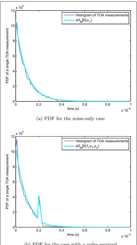
Figure 4 shows an example of the PDF of a single FP pulse arrival time measurement in the case of (20) and (21), respectively, which were fitted to the histogram of TOA measurements. Figure 4a is obtained under the condition offL = 3.1 GHz,fH = 6.1 GHz,VN/σB= 1.7, where the

horizontal axes indicates the measured TOA, and Fig.4b is obtained when the FP arrives attr = 2 ns with a

first-peak-to-noise-ratio (FPNR) ofFPNR = 0.5 dB based on the noise floor in Fig. 4a, whereFPNR=10 logA2_/σ2

B

(7)

Fig. 4PDF of the threshold-crossing moment forathe noise-only case,bthe case with a single received FP pulse attr=2 ns and

FPNR₌0.5 dB. The bandpass noise signal is white within fL=3.1 GHz andfH=6.1 GHz andVN/σB=1.7

early false alarm (PEFA), probability of detection (PD), and

probability of missed detection (PMD) as

PEFA= { probability of a TOA measurement which

occurs in the time interval before the FP pulse arrives},

PD= { probability of a TOA measurement which

occurs in the time interval of the FP pulse}, PMD= { probability of a TOA measurement which

occurs in the time interval after the FP pulse}.

Accordingly, we can get the equations for these probabilities as

PEFA= _t_r

0

pe(tM[k] ;μ1)dtM[k]=1−e−μ1tr,

PD= tf

tr

pd(tM[k] ;tr,μ1,μ2)dtM[k]

=e−μ1tr₁−_e−μ2tw_,

PMD = ∞

tf

pm(tM[k] ;tr,μ1,μ2)dtM[k]

=e−μ1tr_e−μ2tw_,

(22)

wheretw=tf −tr.

Moreover,PEFAandPMDcan both be categorized asPFA;

thus, we havePFA=PEFA+PMD.

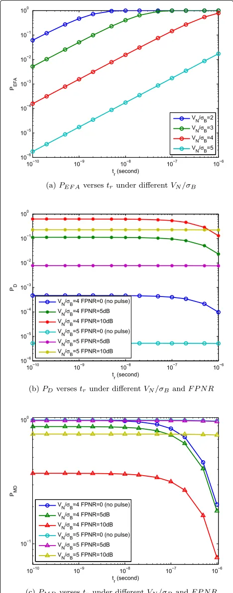
Based on (22), Fig. 5 gives an overview on how the variablestr,VN/σB, andFPNRaffectPEFA,PD andPMD.

Specifically, Fig. 5 indicates that the interval between the start of the measurement and the arrival time of the pulse trhas a significant influence onPEFA,PD, andPMDbesides

of the obvious impact ofVN/σB andFPNRas discussed

in [1] and [2]. Figure 5a and (22) show thatVN/σB and tr are factors which would influence PEFA. PEFA is the

probability of triggering by noise which increases withtr.

Moreover,μ1in (22), which depends onVN/σB

accord-ing to (17) and (20), determinesPEFA, and a lowerVN/σB

results in largerPEFAbecause at a lowerVN, level-crossing

by noise becomes more likely. Figure 5b indicates that FPNR,VN/σB, and tr influencePD. For a fixed FPNR, a

lowerVN/σBresults in a larger negative slope inPDwhich

increases withtrbecause of the increasedPEFA, and larger FPNRleads to a higherPD for a fixed VN/σB. This can

be explained as, whenVN is lower, the input signal has

a larger probability to crossVN, while whentr is larger, PEFA increases due to the increased probability of

trig-gering due to noise before the pulse has arrived. For the sameVN/σB, a largerFPNRwill increase PD, since for a

larger amplitude of the FP pulse it will be more likely to be detected. Similarly, Fig. 5c shows the relation between FPNR,VN/σB,tr, andPMD that FPNRandVN/σB

influ-ence the initial offset of PMD and VN/σB has a major

impact on the slope ofPMD.

3.3 Composite hypothesis testing

Since the distribution of the measured level-crossing times in the noise-only case (FPNR=0) is different from that in case a pulse is present (FPNR = 0), as shown in Fig. 4, this characteristic can be exploited in detection of the pulse from the noise floor using composite hypothesis testing.

3.3.1 The GLRT detector

(8)

Fig. 5Relation betweenPEFA,PDandPMDas a function of the true FP

arrival timetr, and the parametersVN/σBandFPNRas deduced from

(22)

tM[ 1]≤ · · ·tM[k]≤ · · · ≤tM[K] (k=1,· · ·,K), wherep

andqare the number of measurements which are located in the time interval 0 < tM[k]< tr and tr ≤ tM[k]≤ tf, respectively, i.e., p+ q ≤ K. Now, we consider the

following two hypotheses

H0:μ1=μ2, noise-only case (A=0) ,

H1:μ1=μ2, pulse received case (A>0 orA<0) . A GLRT detector decidesH1if

L(tM)=

p(tM;ˆtr,μˆ1,μˆ2,H1) p(tM;μˆ1,H0) = max

tr,μ1,μ2

p(tM;tr,μ1,μ2,H1) p(tM;μ1,H0) > γ

, (23)

whereˆtris the MLE of the TOA underH1,γ is the thresh-old of the GLRT detector andp(tM)is the joint PDF of

(21), which is

p(tM;μ1,H0)= K

k=1

pe(tM[k] ;μ1),

p(tM;tr,μ1,μ2,H1)= p

k=1

pe(tM[k] ;μ1)·

p+q

k=p+1

pd(tM[k] ;tr,μ1,μ2)·

K

k=p+q+1

pm(tM[k] ;tr,μ1,μ2),

where·is the multiplication operator.

Furthermore, whenσ₀2is unknown,μˆ1 andμˆ2can be obtained by fittingPEFAandPDto the empirical statistics

of the TOA measurements as follows

PEFA= tr

0

pe(tM[k] ;μˆ1)dtM[k]= p K ,

PD= tf

tr

pd(tM[k] ;tr,μˆ1,μˆ2)dtM[k]= q K .

(24)

The final estimated TOAˆtris found by maximizing (23)

over all possible values of tr [25]. The search step of tr

can be chosen according to the resolution oftM[k]. To be

specific, during every search step oftr,p, andqare first

calculated and thenμˆ1andμˆ2are obtained from (24).

3.3.2 The optimal GLRT detector

In (23), the threshold of the detectorγis to be determined. In order to optimize the setting ofγ, we use the idea of the Neyman-Pearson lemma, which is based on a single observation, for multiple observations. And chooseγ by setting the probability of false alarmPFAequal toα, as

PFA=

{tM:L(tM)>γ}

(9)

Let u(k) = tM[k]−ˆtr, (k=p+1,· · ·,p+q), where u(k) conforms to a truncated exponential distribution u(k)∼Exp(μˆ1), u(k)∈(0,tw). Set the test statisticT= p+q

k=p+1u(k). The critical region{tM:L(tM) > γ}in (25) can be deduced toT ≶ γ(see Appendix). Accordingly, (25) can be re-written as

PFA=

{T≶γ}

p(T;μˆ1,H0)dT =α. (26)

Bain and Weeks [26] indicates that the PDF of p(T;μˆ1,H0)is given by

3.3.3 Joint PDF approximation approach

Since the calculation of (27) has the potential risk of overflowing machine precision whenqis large, an approx-imation of (27) can be used as a sub-optimal solution in practice.

Monte Carlo simulation based on the empirical his-togram ofT shows thatp(T;μˆ1,H0)can be fitted to the Erlang distributionT ∼Erlang(Ap,Bt)or the Normal dis-tributionT ∼Normal(Mu,Sig), whereApandBtare the shape and the rate of the Erlang distribution, respectively, andMu andSig are the mean and standard deviation of the Normal distribution, respectively. These parameters can be calibrated from ance ofu(k), respectively, which can be obtained by

E(u(k))=

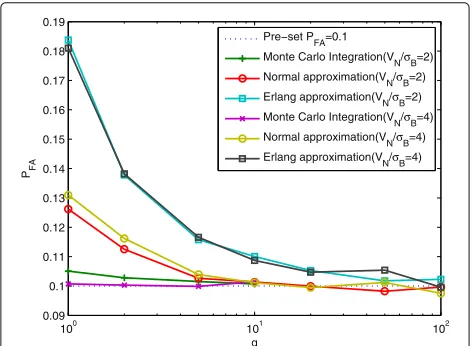
Under these approximations, the goodness of fit of the Erlang approximation and the Normal approximation were tested using Monte Carlo integration [27]. Accord-ing to (26), the pre-setPFA =α leads to a corresponding

thresholdγby means of calculating the inverse cumula-tive density function (CDF) ofT. However, aγcould be biased due to the approximation of p(T;μˆ1,H0), which would lead to a biasedPFA accordingly, compared to the

usage of the truep(T;μˆ1,H0). Since (27) is only obtain-able whenqis small, we takePFAobtained by Monte Carlo

integration as a reference to evaluate these two possible approximations. Figure 6 shows the results of the bias in PFA forVN/σB = 2 (lowVN/σB case) andVN/σB = 4

(desiredVN/σBcase), where the bias inPFAunder the two

approximations are compared to thePFA obtained from

the Monte Carlo integration. It is seen that, whenqis large enough (q > 10), it is feasible to use either the Normal or the Erlang distribution to approximate p(T;μˆ1,H0) in (27) with less than 1% bias in PFA under the given

conditions.

Monte Carlo Integration(V_N/σB=2)

Normal approximation(V_N/σB=2)

Erlang approximation(V_N/σB=2)

Monte Carlo Integration(V_N/σB=4)

Normal approximation(V_N/σB=4)

Erlang approximation(V_N/σB=4)

Fig. 6Comparison of the joint PDF approximation tests showing the bias inPFAdue to the joint PDF approximation (Erlang approximation

(10)

4 Simulation results

In the simulations, we use the following parameters: a BPF withfL = 3.1 GHz andfH = 6.1 GHz, i.e.,fc = 4.6 GHz

andB = 3 GHz, the number of measured arrival time eventsK = 100, PFA = 0.1, and the resolution of each

recorded TOA measurement is assumed to be 10 ps. The TOA estimation results are shown in Figs. 7, 8, and 9, where the horizontal axis indicates the true TOAtr and

the vertical axis gives the mean absolute estimation error. In [2], the measurement window is devided in a number of time bins. It is shown that the TOAtris within the first

time bin of the measurement window which contains at leastKTHout ofKmeasured TOA’s, where 1≤KTH≤K.

Specifically, a 160 ns time window at the start of each mea-surement window is excluded from the analysis because of the high probability of triggering due to noise. The ratioVN/σB∈[ 3.5, 5.5] is selected according to the chosen

bounds onPEFAandPMD.

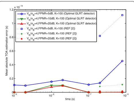
The results of Fig.7 show that under the conditions where VN/σB and FPNR are set relatively high, both

the proposed GLRT detector-based TOA estimation and the time-window-based TOA estimation from [2], realize centimeter-level ranging accuracy. The TOA estimation scheme proposed in this paper shows improved perfor-mance compared to the scheme used in [2].

Compared to [2], the GLRT-based pulse detection and TOA estimation scheme works in the whole measure-ments window, without any unreachable time range as shown in Fig. 7, for this scheme detects the pulse as well as estimates its arrival time based on the ratio of the PDFs of the pulse-present case and noise-only case. Since in [2] the start of the measurement period is discarded from the

10−9 10−8 10−7 10−6

0 0.2 0.4 0.6 0.8 1 1.2x 10

−10

time (s)

Mean absolute TOA estimation error (s)

V_N/σB=4,FPNR=5dB, K=100 (Optimal GLRT detector)

V_N/σB=4,FPNR=5dB, K=100 (REF [2])

Fig. 7TOA estimation error forVN/σB=4 withFPNRas parameter.

This figure compares the TOA estimation error between the proposed GLRT detector and the time-window-based detector of [2] with the true TOAtrranging from 1 ns to 1μs, where the time-window-based

detector only works in thetrrange from 160 ns to 1μs

10−9 10−8 10−7 10−6

10−13 10−12 10−11 10−10 10−9 10−8 10−7 10−6

time (s)

V_N/σB=2,FPNR=5dB, K=100

Fig. 8TOA estimation error for lowVN/σBwithFPNRas parameter

measurements, a pulse cannot be detected when it arrives within this 160 ns window. The improved performance of the proposed technique is because it is an MLE scheme based on the PDFs of the measured data, rather than a time-window-oriented detection scheme, which better exploits the available information of the measurement data. But this comes at the expense of a higher compu-tational cost. Moreover, the proposed scheme could work under a wider range ofVN/σBandFPNRunder specific

conditions (e.g., specific range oftr), as shown in Figs. 8

and 9, which is not applicable for the scheme in [2]. Figure 8 shows the performance of the proposed scheme for lower values of VN/σB. For the cases of VN/σB =

2 and 3, it is observed that the TOA estimation error increases with increasingtr. This is due to the fact that PEFAincreases and andPDdecreases with increasingtras

shown in Fig. 5a, b, respectively. Also,PDdecreases faster

for smallerVN/σB.

10−9 10−8 10−7 10−6

10−12 10−11 10−10 10−9 10−8 10−7 10−6

time (s)

V

N/σB=3,FPNR=0dB, K=100

V

(11)

Figure 9 shows the TOA estimation accuracy when receiving a weak pulse signal. In case of highVN/σBand lowFPNRwhereVN/σB = 4 and 5 andFPNR = 0 dB, the thresholdVTH shown in (3) is relatively high

com-pared toσB, resulting in a low probability of detection of the FP pulse, but instead triggering of the detector hap-pens mainly due to noise, i.e., resulting in EFAs and MDs. For lowVN/σBand lowFPNR, e.g., withVN/σB=2 and 3

andFPNR=0 dB, it is possible to still detect the FP pulse, even whentr is relatively small, because it has a larger

probability to cross the lowerVN. However, due to the low VN/σB, a large fraction of the threshold crossings will be

due to noise and cause EFAs whentrincreases; therefore,

the TOA estimation error is higher.

By comparing Figs. 7, 8, and 9, we find the trade-off between the sensitivity of the receiver and the accuracy of TOA estimation. When settingVN/σBhigh, a more

accu-rate estimation can be obtained for highFPNR, as shown in Fig. 7. However, a high VN/σB also causes the

miss-ing of weak FP signals, as shown in Fig. 9. On the other hand, a lowVN/σBsetting will increase the sensitivity of the receiver but it worsens the estimation accuracy, espe-cially whentris large, as shown in Figs. 8 and 9. In general,

the above analysis provides an approach to an optimal trade-off by selecting relatively low VN/σB according to

the expected range oftr, so as to realize centimeter-level

TOA estimation accuracy.

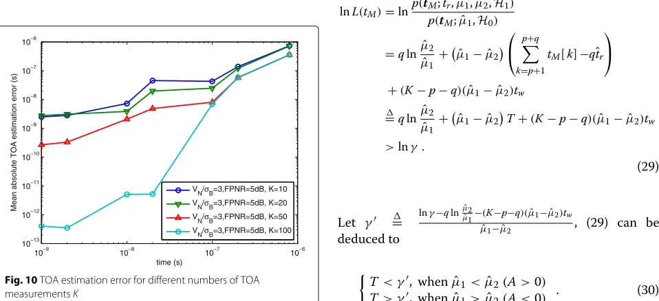
In Fig. 10, the effect of the numberKof TOA measure-ments on the TOA estimation accuracy is shown while keeping VN/σB and FPNR constant. It is observed that

the TOA estimation accuracy improves with increasingK. This is because the unknown parameters μ1 and μ2 in the GLRT detector are estimated from the empirical his-togram deduced from the number of TOA measurements by (24). Therefore, the estimation accuracy ofμ1andμ2as

10−9 10−8 10−7 10−6

V

Fig. 10TOA estimation error for different numbers of TOA measurementsK

well astr are improved when the number of the collected

samples is larger.

5 Conclusions

An improved TOA estimation scheme for UWB pulse sig-nals is proposed for a sub-Nyquist sampling receiver based on first-threshold-level crossing using statistical analysis of a number of measured arrival time events. The thresh-old crossing procedure of the receiver for the noise-only case and the case when a pulse plus noise is received has been unified to a common first-crossing problem in a continuous random process. Based on this mathemati-cal model, the PDF of the arrival time events was deduced under two categories of receiver bandwidth. An analysis is given on how to estimate the PSD of the noiseσ₀2based on empirical measurement data and how the parameters threshold to band-limited noise deviation-ratio VN/σB,

first-peak-to-noise-ratio FPNR, and true TOA tr affect

the probability of early false alarm PEFA, probability of

detectionPD, and probability of missed detection PMD.

For estimation of the TOA from a number of measured arrival time events, a composite hypothesis test and MLE is applied. Compared to the TOA estimation strategy used in [2], this pulse detection and TOA estimation approach make use of the PDF of TOA measurements data instead of statistical data on probability; therefore, more informa-tion is obtained and exploited, resulting in a more accurate TOA estimation within a wider time frame range.

Appendix

Proof of the critical region transformation in NP lemma strategy

The critical region in (25) is

(12)

Acknowledgements

This research work is founded by the NWO HERE-2 project (No. 11951).

Authors’ contributions

YX made the main contributions to the theorems, implementations, and drafting this paper. GJ is the advisor who directed this work and contributed to the theorems and revisions. SS and CT contributed to the GLRT detector part and revisions. All authors read and approved the final manuscript.

Competing interests

The authors declare that they have no competing interests.

Publisher’s Note

Springer Nature remains neutral with regard to jurisdictional claims in published maps and institutional affiliations.

Author details

1_{Faculty of Electrical Engineering, Mathematics and Computer Science, Delft}

University of Technology, Mekelweg 4, 2628 CD Delft, The Netherlands. 2_{Faculty of Civil Engineering and Geosciences, Delft University of Technology,}

Stevinweg 1, 2628 CN Delft, The Netherlands.

Received: 15 May 2017 Accepted: 31 August 2017

References

1. I Guvenc, Z Sahinoglu, Threshold selection for UWB TOA estimation based on kurtosis analysis. IEEE Commun. Lett.9(12), 1025–1027 (2005) 2. G Bellusci, GJM Janssen, J Yan, CCJM Tiberius, Performance evaluation of a

low-complexity receiver concept for TOA-based ultrawideband ranging. IEEE Trans. Veh. Technol.61(9), 3825–3837 (2012). doi:10.1109/TVT.2012.2207749 3. J-Y Lee, RA Scholtz, Ranging in a dense multipath environment using an

UWB radio link. IEEE J. Sel. Areas in Commun.20(9), 1677–1683 (2002). doi:10.1109/JSAC.2002.805060

4. C Falsi, D Dardari, L Mucchi, MZ Win, Time of arrival estimation for UWB localizers in realistic environments. EURASIP J. Advances in Sig. Process.

2006(1), 032082 (2006)

5. V Lottici, A D’Andrea, U Mengali, Channel estimation for ultra-wideband communications. IEEE J. Sel. Areas in Commun.20(9), 1638–1645 (2002) 6. H Boujemaa, M Siala, inCommunications, 2001. ICC 2001. IEEE International

Conference On. On a maximum likelihood delay acquisition algorithm, vol. 8 (IEEE, 2001), pp. 2510–2514

7. Z Sahinoglu, S Gezici, I Guvenc,Ultra-wideband positioning systems theoretical limits, ranging algorithms, and protocols. (Cambridge Univerisity Press, 2008). www.cambridge.org/9780521873093

8. SJ Howard, K Pahlavan, Measurement and analysis of the indoor radio channel in the frequency domain. IEEE Trans. Instrum. Meas.39(5), 751–755 (1990)

9. K Pahlavan, P Krishnamurthy, A Beneat, Wideband radio propagation modeling for indoor geolocation applications. IEEE Commun. Mag.36(4), 60–65 (1998)

10. SS Ghassemzadeh, R Jana, CW Rice, W Turin, V Tarokh, Measurement and modeling of an ultra-wide bandwidth indoor channel. IEEE Trans. Commun.52(10), 1786–1796 (2004)

11. C-C Chong, SK Yong, A generic statistical-based UWB channel model for high-rise apartments. IEEE Trans. Antennas Propag.53(8), 2389–2399 (2005)

12. Z Tarique, W Malik, D Edwards, Bandwidth requirements for accurate detection of direct path in multipath environment. Electron. Lett.42(2), 100–102 (2006)

13. NA Alsindi, B Alavi, K Pahlavan, Measurement and modeling of ultrawideband TOA-based ranging in indoor multipath environments. IEEE Trans. Veh. Technol.58(3), 1046–1058 (2009)

14. X Li, K Pahlavan, Super-resolution TOA estimation with diversity for indoor geolocation. IEEE Trans. Wirel. Commun.3(1), 224–234 (2004)

15. H Saarnisaari, inVehicular Technology Conference, 1997, IEEE 47th. TLS-ESPRIT in a time delay estimation, vol. 3 (IEEE, 1997), pp. 1619–1623 16. JL Paredes, GR Arce, Z Wang, Ultra-wideband compressed sensing:

channel estimation. IEEE J. Sel. Top. Sig. Process.1(3), 383–395 (2007). doi:10.1109/JSTSP.2007.906657

17. V Yajnanarayana, P Handel, Compressive sampling based UWB TOA estimator. arXiv preprint arXiv:1602.08615 (2016)

18. RJ Fontana, SJ Gunderson, inUltra Wideband Systems and Technologies, 2002. Digest of Papers. 2002 IEEE Conference On. Ultra-wideband precision asset location system (IEEE, 2002), pp. 147–150

19. G Bellusci, GJM Janssen, J Yan, CCJM Tiberius, in2009 IEEE International Conference on Ultra-Wideband. A low-complexity UWB receiver concept for TOA based indoor ranging, (2009), pp. 618–623. doi:10.1109/ICUWB.2009.5288687 20. G Bellusci, G Janssen, J Yan, C Tiberius, inProceedings of the 22nd

International Technical Meeting of The Satellite Division of the Institute of Navigation (ION GNSS 2009). A sub-sampling receiver architecture for ultra-wideband time of arrival based ranging, (2009), pp. 471–480 21. JR Rice, FP Beer, First-occurrence time of high-level crossings in a

continuous random process. J. Acoust. Soc. Am.39(2), 323–335 (1966). ASA. http://asa.scitation.org/doi/abs/10.1121/1.1909893

22. SO Rice,Mathematical Analysis of Random Noise. ([New York] : American Telephone and Telegraph Co, New York, 1944)

23. JS Bendat, AG Piersol,Random data: analysis and measurement procedures, Fourth Edition. (John Wiley & Sons, Inc., New Jersey, 2012), pp. 109–171. doi:10.1002/9781118032428.ch5

24. SH Crandall, KL Chandiramani, RG Cook, Some first-passage problems in random vibration. J. Appl. Mech.33, 532 (1966). doi:10.1115/1.3625118 25. SM Kay,Fundamentals of statistical signal processing: detection theory.

Prentice Hall Signal Processing Series. (Prentice-Hall PTR, New Jersey, 1998) 26. LJ Bain, DL Weeks, A note on the truncated exponential distribution. Ann.

Math. Statist.35(3), 1366–1367 (1964). doi:10.1214/aoms/1177703298 27. PJG Teunissen, DG Simons, CCJM Tiberius,Probability and observation