Application of a weighted likelihood method to hypocenter determination
M. Imoto
National Research Institute for Earth Science and Disaster Prevention, 3-1 Ten-nodai, Tsukuba, Ibaraki 305-0006, Japan
(Received June 25, 2012; Revised July 25, 2013; Accepted July 28, 2013; Online published December 6, 2013)
The method of least squares is a standard approach to hypocenter determination in seismology. However, this method is not useful for data contaminated by systematic errors. To address this problem, we propose a weighted likelihood method (WLL) rather than a weighted least-squares method (WLSQ). Assuming a normally distributed random error and systematic errors, both methods give the same solution; however, variances of random errors estimated by WLSQ are much smaller than those estimated by WLL. Examining reasonable random errors, we simulate a case of systematic errors varying linearly with a given parameter, where the number of unknown parameters is reduced to one for simplification. We assume that a systematic error, two different arrays of stations, and three different weights are functions of distance. In the cases where biases affected by systematic errors are adequately reduced, the variances of random errors estimated by WLL become roughly equal to that assumed, but those estimated by WLSQ are much smaller than that assumed. This result implies that WLL is a better approach than WLSQ for data contaminated by systematic errors.
Key words:Weighted likelihood method, weighted least squares, hypocenter determination, systematic error.
1.
Introduction
The method of least squares is a standard approach to the approximate solution of overdetermined systems. Use of this method can reduce the effect of random errors. The best solution in the least-squares method minimizes the sum of squared residuals—a residual being the difference between an observed value (arrival time of a seismic wave) and the fitted value provided by a model (origin time and location of an earthquake and a seismic velocity model). Hypocenter determination employs the nonlinear least squares method and is implemented by iterative refinement. If it is assumed that random error variances largely vary among observation stations, the weighted least-squares method (WLSQ) can be used to determine the hypocenter more reliably.
The residual is caused by both errors in the measurement of the arrival time and errors in the seismic velocity model for calculating theoretical arrival times. The former is a ran-dom error, but the latter is a systematic one. For a nation-wide network in Japan, such as those operated by the Japan Meteorological Agency (JMA) and the National Research Institute for Earth Science and Disaster Prevention (NIED), a simple velocity model for hypocenter determination of-ten involves systematic errors in the calculated travel time, since seismic velocities vary from region to region. JMA and NIED currently adopt WLSQ, in which the weight of each observation depends on its hypocentral distance. Their procedure, which may be a better approach than a simple least-squares method, obviously violates the condition that the least-squares method must be applied to data without systematic errors. Therefore, this procedure may give
unre-Copyright cThe Society of Geomagnetism and Earth, Planetary and Space Sci-ences (SGEPSS); The Seismological Society of Japan; The Volcanological Society of Japan; The Geodetic Society of Japan; The Japanese Society for Planetary Sci-ences; TERRAPUB.
doi:10.5047/eps.2013.07.010
liable solutions, which has not yet been addressed.
In this study, we presume both normally distributed ran-dom errors and systematic errors and propose the use of the weighted likelihood method (WLL) (Hu and Zidek, 2002; Wang and Zidek, 2005) to address this problem. First, we demonstrate that WLSQ and WLL provide the same solu-tion; however, the variance of random errors estimated by WLL exceeds that estimated by WLSQ. In order to clarify which method estimates more reasonable errors, both meth-ods are applied to data contaminated with systematic errors in order to simulate hypocenter determination with an un-suitable velocity model. The solutions with both methods could be analytically obtained for the simulated data. This paper compares the variance of random errors estimated by the maximum likelihood method with the assumed ones. This comparison indicates that WLSQ underestimates the variance of the random errors and is unreliable as an ap-proach to this problem.
2.
Method
2.1 Weighted least squares
The simple least-squares method assumes that the stan-dard deviation of the random error is constant for all sam-ples. When the standard deviation varies, WLSQ can be applied. Less weight is given to less precise measurements, and more weight is given to more precise measurements.
Here,σ andσidenote the standard deviation of the random
error in a representative observation and theith observation
(i =1, . . .n), respectively. The weightwiis inversely pro-portional to the variance of the error, and is represented by
σ2/σ2
i. The likelihood function in this case is given as:
L=
n
i=1 ⎡ ⎣ 1
2πσ2
i exp
− 1
2σi2
(oi−ci)2 ⎤
⎦
=
where oi denotes the observed value and ci denotes the
theoretical value at thei-th observation.
The maximum log-likelihood is obtained as:
lnLmax= −
where the subscript WLSQ refers to the weighted least-squares method.
2.2 Weighted likelihood method
If reliabilities of observed samples differ from sample to sample, each sample can contribute to the maximum likeli-hood estimate in proportion to its reliability through WLL. The WLL function is given in the form of the weighted sum of log-likelihoods for each sample:
lnL =
The maximum log-likelihood is obtained as:
lnLmax= −
where the subscript WLL refers to the weighted likelihood method.
When the same weights are applied in WLL and in
WLSQ, the same solutions of ci are obtained. However,
the maximum likelihood estimates ofσ2are different.
3.
Simulation
In applying WLL to hypocenter determination, the only
difference from WLSQ is related to the formula for σ2,
where Eq. (10) can be compared with Eq. (5). When NIED and JMA determine the hypocenter, a weight with epicen-tral distance may be introduced to reduce bias due to sys-tematic errors in the calculated travel times. The structure of seismic wave velocities in Japan cannot be modeled with a simple layered structure, as employed by NIED and JMA. Therefore, using arrival times of more distant stations in the determination results in systematic errors, and bias of the determined hypocenter. In this section, we examine which of WLSQ or WLL is better for hypocenter determination af-fected by systematic errors from an inappropriate velocity structure.
We schematically simulate this problem assuming simple conditions. We assume that an earthquake occurs on the surface of a uniform medium and that stations are densely deployed in a line from the epicenter in the first case, and on a two-dimensional surface in the second case. A systematic error due to an inappropriate velocity structure is as large as a random error at a short distance, and becomes much larger at more distant points. It is assumed that the epicenter of the earthquake is rather well constrained but the origin time of the earthquake is not, since the dense stations are well distributed. Thus, the problem of hypocenter determination is reduced to the problem of determining the origin time of the event.
The observed arrival time at theith (i =1,2, ..n) station is
ti =t0+T(ri)+B(ri)+εi, (11)
whereri is the epicentral distance,T(ri)is the travel time
estimated by the model, and B(ri) is a systematic error
due to an inappropriate velocity model. In the single-layer model, this correction must be a function of epicentral dis-tance, seismic wave velocity in the model, and the actual seismic wave velocity:
whereVc is the actual value of the seismic wave velocity,
andVmis the seismic wave velocity used in the model. The
term on the right-hand side is a linear function of epicentral distance:
B(ri)=α·ri. (13)
Equation (11) can be represented as:
ti =t0+T(ri)+α·ri+εi. (14)
As the epicenter is well constrained under our assumption, the epicentral distance is considered to be a known
param-eter. Therefore, subtractingT(ri)from the arrival time, we
considert0 to be an unknown parameter, and Eq. (14) can
be replaced by:
Here, the problem of hypocenter determination is reduced
to the problem of estimatingt0from observationoi
contam-inated by a systematic error and a random error.
Without loss of generality, we fix the true value of the
origin time to be 0. The sum of the residual squares R2is
calculated as:
wherexrefers to the estimated origin time. The maximum
likelihood estimate of the origin time,xˆ, minimizesR2and
is calculated as follows:
ˆ
The minimum ofR2is calculated as:
ˆ
In the present study, we can estimate the expected values of Eqs. (17) and (18) with a probability density function for
the epicentral distance of stations,S(r), and the assumption
that the random error of εi is normally distributed with a
mean 0 and varianceδ2. A weight functionW(r)is applied
and different limits of epicentral distance,u, are considered.
In order to derive an analytical solution of Eq. (17), we assume a two-step random value generation.
Step 1. Random generation ofnstations within a distance
ofu.
Step 2. For each set of stations, generate a large number
(l) of series of random errors, (εi j: where j refers to the
number of trials, j =1,2, ...l).
For thejth trial ofεi j, we obtain the maximum likelihood
estimate of the origin timexˆjas follows:
ˆ
whereεi jrefers to the random error at theith station in the
jth trial. For a large number ofl,xˆjapproachesE(xˆ)as:
whereEdenotes the expected value of a variable, since, for
large enough values ofl,
1
which is an average of independent random errorsεi j
nor-mally distributed with a mean 0. Thus, for each selection of stations, the expected value of Eq. (17) is given by Eq. (21).
For a set of largen, Eq. (21) can be represented as:
Here, we assume thatm stations are distributed within an
epicentral distance of 10 units.
Similarly, the expected value of Eq. (18) is derived as follows. For the jth trial of a set of stations:
ˆ This replacement will be justified by a Monte Carlo
simu-lation. We obtain the average value of Eq. (28) over jfor a
large number ofl:
Equation (29) can be represented by:
E
We analytically estimated the expected values ofxˆ,σˆWLL
andσˆWLSQfor a large number ofnin this way. Hereafter,xˆ,
ˆ
σWLLandσˆWLSQdenote the expected values ofxˆ,σˆWLLand
ˆ
σWLSQ, respectively.
We consider two different observation station arrays and three different weight functions. In one case of the arrays, these stations are distributed in a line (Array1). The density function ofS(r)is given as:
Table 1. Formulas for estimating the values ofA,C, andD. Two different arrays of stations are listed in different columns. Three different weight functions are listed in rows.
S(r)=0.1,m=100 S(r)=0.02r,m=100
In the other case, we consider stations deployed uniformly
in a plane (Array2). The density function of S(r)is given
as
S(r)=0.02r. (33)
Three different weighting functions are considered be-low. For the first case of applying a constant weight, the function ofW(r)is given as:
W(r)=1. (34)
For the second case, where the weight decays inversely as the second power of distance, the weight is given as:
W(r)=
The assumed systematic error, B(r), increases linearly
with epicentral distance. WLSQ likely misapplies a weight-ing function that decays as the inverse of the second order of the epicentral distance, since the square of the system-atic error increases in proportion to the second power of distance.
The last case, where the weight function decays as the inverse of the fourth power of epicentral distance, can be considered as an example of weight decaying faster than in the previous cases:
Table 1 lists formulas estimating the values of A, C,
andDfor each of the six cases. Substituting these values
into Eqs. (23), (30), and (5) or (10), we obtain standard
deviations of random errors, σˆWLSQ for WLSQ and σˆWLL
for WLL.
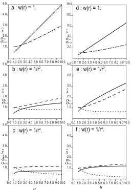
Figures 1(a) through (f) illustratexˆ,σˆWLSQandσˆWLLwith
the upper limitu varying from 1 to 10 units, whereα=1
andδ = 1. The systematic error is assumed to be equal
to, or less than, the random error in a range of 0 to 1 units,
where the weight is fixed to 1.σˆWLSQ(dotted line) andσˆWLL
(dashed line) are compared with the assumed random error
(δ =1). In each set, xˆ represents the bias affected by the
systematic error, since the correct origin time is set to 0. In Figs. 1(a), 1(b), 1(d) and 1(e), biases caused by
sys-tematic errors are not adequately reduced, wherexˆdeparts
from 0. In these cases,σˆWLL exceeds the standard
devia-tion of the assumed random error. In both stadevia-tion arrays, it is clear that the most quickly decaying weight function
(Figs. 1(c) and 1(f)), gives the best solutions, wherexˆ
be-comes at most 1 even in cases including stations up to 10 units away. This suggests that biases are adequately
re-duced. In these cases,σˆWLLbecomes reasonable at around
1, mostly equal to the standard deviation of the assumed
random error. In contrast,σˆWLSQvalues are much smaller
than that assumed. Therefore, WLSQ underestimates the standard deviation of random errors, suggesting an invalid application of WLSQ to the present issue.
Table 2 summarizes xˆ, σˆWLSQ and σˆWLL for u = 10.
Results obtained from the weight function decaying as the inverse of the seventh power are added as a more quickly decaying weight function, which is the case of NIED. In
this case,xˆ andσˆWLLbecome slightly better than those of
other cases, wherexˆbecomes smaller andσˆWLLapproaches
1. These examples suggest that ifσˆWLLexceeds the standard
deviation of the assumed random error, biases caused by systematic errors would not be adequately reduced.
Biasxˆcould not be compared with its standard error, the
derivation of which is based on the Hessian/Fisher
Infor-mation matrix of the log-likelihood function (Sakamotoet
al., 1983), since the standard error ofxˆconcerns only
ran-dom errors, while the bias originates from systematic er-rors. From a quantitative viewpoint, it should be noted that, in our definition,xˆ,σˆWLLandσˆWLSQare functions ofuand are independent ofm, but the standard error ofxˆ,σˆ (σˆWLL
orσˆWLSQ) divided by the square root ofC, is inversely
pro-portional to the square root ofm, which can easily be
veri-fied from Eqs. (5), (10), (23), (24), (25), (26), (30) and (31).
The ratio ofxˆto its standard error becomes large in
propor-tion to the square root ofm. Consequently, biasxˆcannot be
compared with its standard error.
4.
Discussion and Summary
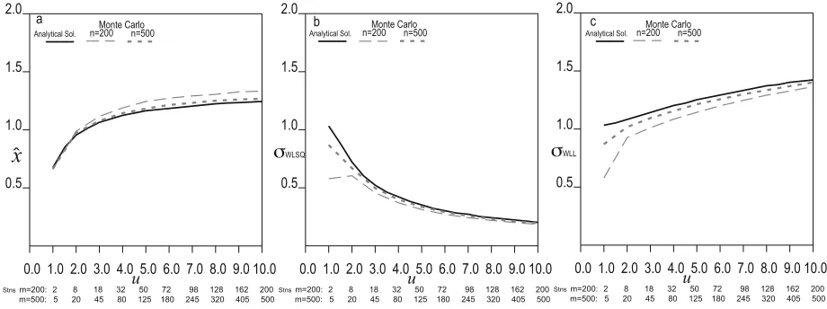
A Monte Carlo simulation was conducted to confirm Eq. (23) and justify the replacement in Eq. (29). Figures 2(a), 2(b) and 2(c) illustratexˆ,σˆWLSQandσˆWLLvalues ob-tained for the set of Fig. 1(f). For each distance limit, the
number of stations can be calculated byS(r), and their
lo-cations are randomly generated. Random errors are also
Fig. 1. Variation ofxˆ,σˆWLLandσˆWLSQ. The time scale (ordinate) is measured in a unit ofδ. The solid, dashed and dotted curves denotexˆ,σˆWLLand
ˆ
σWLSQ, respectively. Figures 1(a), 1(b), 1(c). Different weight functions with Array 1. Figures 1(d), 1(e), 1(f). Different weight functions with Array
2. In Figs. 1(a) and 1(d), the dotted and dashed curves completely overlap each other.
Table 2. List ofxˆ,σˆWLSQandσˆWLL. The listed values are estimated by stations at distances of up to 10 units. Results from the 7th power are also listed.
S(r) Power ofw(r) xˆ σˆWLSQ σˆWLL
Array1
0 5.00 3.06 3.06
−2 1.48 0.84 1.93
−4 0.75 0.43 1.17
−7 0.60 0.36 1.07
Array2
0 6.67 2.56 2.56
−2 3.33 0.66 2.77
−4 1.24 0.20 1.42
−7 0.83 0.13 1.07
Eqs. (20) and (29). Ten thousand sets of stations are gener-ated for each distance limit, which is shifted from 1 to 10 units for every unit step. In each set of the figure, the simple
averages over ten thousand sets form=200 (dashed line)
andm = 500 (dotted line) are compared with analytical
solutions (solid line).
In general, as the number of stations increases (fixed dis-tance limit), the results obtained by the simulation approach those of the analytical solution. Qualitative relations among
ˆ
x,σˆWLLandσˆWLSQobtained from the Monte Carlo
simula-tion do not largely differ from those of the analytical solu-tions, except in the case of a few tens of stations. Although
not shown here, the agreement between the simulation and the analytical solution in other cases (the other station array and/or different weights) becomes better than that of Fig. 2. We have only discussed qualitative relations between the parameters, so an analytical solution is an appropriate ap-proach to this issue.
epi-Fig. 2. Results obtained by the Monte Carlo simulation are compared with the analytical solution for the set of epi-Fig. 1(f). Figures 2(a), 2(b) and 2(c) illustratexˆ,σˆWLSQandσˆWLLvalues, respectively. In each set, the simple averages over ten thousand sets form=200 (dashed curve) andm=500
(dotted curve) are compared with the analytical solution (solid curve). The number of stations within each distance limit is indicated.
central/hypocentral distance, which originate from the dif-ference in velocity structure between the model used in hypocenter determination and the actual case. In order to reduce this bias, NIED (Shiomi, 2009 (personal communi-cation)) introduced a weight depending on the hypocentral distance,Y:
W(Y)=Ymin7 /Y7,
whereYminis the hypocentral distance of the station closest
to the hypocenter (km) (ifYmin ≤ 50, thenYmin = 50; if
W(Y) >1, thenW(Y)=1).
However, JMA introduced a similar weighting depending on the hypocentral distance except for the order of power:
ForP-waves (Wp):Wp =Ymin2 /Y2
ForS-waves (Ws):Ws =Wp/3.
Comparing weights in these methods with those of our simulation indicates that NIED, using a weight function de-caying faster than the inverse fourth power, probably suc-ceeds in reducing the bias by systematic errors (Table 2). But, JMA may fail to reduce bias with a weight func-tion decaying inversely with the second power of distance. Both NIED and JMA must underestimate standard errors of
hypocenters, which are calculated based onσˆWLSQ.
Stan-dard errors of hypocenters are often critical in considering reliable hypocenter distributions of clustering earthquakes and their tectonic implications.
For deeper earthquakes, a qualitative consideration could be given as follows. At short epicentral distances compared with the focal depth, systematic errors reach a level depend-ing on the focal depth. On the other hand, at longer dis-tances, systematic errors increase with distance mostly sim-ilar to those of shallow earthquakes. These result in smaller variances of residuals than those of shallower earthquakes, since a range of systematic errors becomes smaller than those of shallower earthquakes. This implies that a
signifi-cant bias may remain, even ifσˆWLL2 approaches the variance
of random error. Such aspects should be discussed further as separate studies, since station arrays, the number of un-known parameters, and other factors must be rearranged to address these issues.
The present paper focuses on only the preliminary
formu-lation of applying WLL to hypocenter determinations. In practical applications of WLL, an optimal weight function should be determined taking into consideration the results in the case of various kinds of earthquakes in different areas and depths (Hu and Zidek, 2002). WLL can be applied to hypocenter determination with a minor revision of current methods which are based on misapplications of WLSQ.
We propose the use of WLL rather than WLSQ for hypocenter determination. Both methods give the same so-lution; however, the variance estimated by WLSQ is much smaller than that estimated by WLL. Our simulation indi-cates that a weight function that decays faster with distance gives a better solution, which could be realized by WLL. In contrast, such flexible weight functions are not justified by WLSQ, since weights should be inversely proportional to the variances of errors. In the cases where biases affected by systematic errors are adequately reduced, the variances of random errors estimated by WLL become roughly equal to the given one, but those estimated by WLSQ are much smaller than the given one. Therefore, WLSQ should not be used to address systematic errors in hypocenter determi-nation. We conclude that WLL is a better approach than WLSQ for data contaminated by systematic errors.
Acknowledgments. The author thanks two anonymous reviewers for their critical reading and comments on this manuscript.
References
Hu, F. and J. V. Zidek, The weighted likelihood,Can. J. Stat.,30, 347–371, 2002.
Japan Meteorological Agency, Users’ Guide, http://data.sokki. jmbsc.or.jp/cdrom/seismological/catalog/notes e.htm (as of April 1, 2013).
Sakamoto, Y., M. Ishiguro, and G. Kitagawa,Akaike Information Criterion Statistics, 290 pp, D. Reidel, Dordrecht, 1983.
Ueno, H., S. Hatakeyama, J. Funakaki, and N. Hamada, Improvement of hypocenter determination procedures in the Japan Meteorological Agency,Quart. J. Seismol.,65, 123–131, 2002 (in Japanese). Wang, X. and J. V. Zidek, Derivation of mixture distributions and weighted
likelihood function as minimizers of KL-divergence subject to con-straints,Ann. Inst. Statist. Math.,57, 687–701, 2005.