A method for simultaneous velocity and density inversion and its application to
exploration of subsurface structure beneath Izu-Oshima volcano, Japan
Shin’ya Onizawa1, Hitoshi Mikada2, Hidefumi Watanabe3, and Shikou Sakashita3
1Institute of Seismology and Volcanology, Graduate School of Science, Hokkaido University, 060-0810, Japan 2Deep Sea Research Department, Japan Marine Science and Technology Center, 237-0061, Japan
3Earthquake Research Institute, University of Tokyo, 113-0032, Japan
(Received June 26, 2001; Revised July 22, 2002; Accepted July 22, 2002)
We have developed a method for three-dimensional simultaneous velocity and density inversion using traveltimes of local earthquakes and gravity data. The purpose of this method is to constrain the velocity inversion and increase the spatial resolution of shallow velocity structures by introducing additional gravity data. The gravity data contributes to the P- and S-wave velocity models by imposing constraints between seismic velocities and density. The constraint curve is constructed so as to fit the data for porous rock samples, and deviations from the curve are taken into account in the inversion. The constraint is imposed at only the first layer, because density structure is well resolved at shallower parts and it is difficult to determine uniquely at greater depths. Synthetic inversion tests indicate that gravity data can improve the resolution of the velocity models for this layer. The method is applied to investigate the subsurface structure of Izu-Oshima volcano, Japan and velocity structures with high spatial resolution are obtained. The additional gravity data contribute primarily to improvement of the S-wave velocity model. At 0.25 km depth, a high velocity anomaly due to caldera-filling lava flows is observed. At 1.25 and 2.5 km depths, high velocity intrusive bodies are detected. A NW-SE trending high velocity belt at 1.25 km depth is interpreted as being caused by repeated intrusion of dikes.
1.
Introduction
In order to understand volcanic activity, it is important to derive the subsurface structure. Inversion for three-dimensional velocity structure has been widely used to in-vestigate subsurface structure beneath volcanoes. At shal-low depths, however, it is difficult to constrain the structure beneath stations with high spatial resolution, though larger heterogeneity is anticipated. This is due to lack of inter-section among seismic rays, since the rays concentrate be-neath seismic stations with a dominantly vertical orientation. This problem is more pronounced when seismic stations are sparsely deployed. In general, gravity observations can be carried out more densely than seismic observations. Thus, at shallow depths, the density structure can be obtained at a higher resolution than the velocity structure. This implies that the velocity inversion can be constrained and spatial res-olution of the velocity structure can be increased by appro-priate use of additional gravity data.
A velocity inversion constrained by gravity data was per-formed by Lees and VanDecar (1991). They assumed the linear relationship between P-wave velocity and density pro-posed by Birch (1961) at blocks in a target region, and strictly fixed this relationship. Thus, unknown parameters could be represented only by slowness perturbations. How-ever, Birch’s relationship is not appropriate for porous rocks commonly found in the shallow parts of volcanoes. Thus, a
Copy right cThe Society of Geomagnetism and Earth, Planetary and Space Sciences (SGEPSS); The Seismological Society of Japan; The Volcanological Society of Japan; The Geodetic Society of Japan; The Japanese Society for Planetary Sciences.
relationship appropriate for shallow porous rocks should be introduced. Furthermore, it is preferable that the relation-ship between velocity and density not be fixed, to allow for deviations that better model the real earth.
Izu-Oshima is one of the most active volcanoes in Japan and the latest eruptive event occurred in 1986–1987. Be-cause of its high activity, many geological and geophysical studies have been conducted. The velocity structure has been investigated by previous research, some studies directed to-ward investigating shallow crustal structure, and some di-rected toward detecting magmatic bodies (e.g., Hasegawaet al., 1987; Yamamoto, 1993; Mikada, 1994). A consistent result from these studies is that a high velocity zone exists beneath the caldera to a depth of about 2 km below sea level. However, other results are not necessarily consistent with each other, and we have therefore been unable to derive a complete description of the magma plumbing system.
There are two purposes to this study. One is to develop a method for three-dimensional simultaneous velocity and density inversion combining traveltime data of local earth-quakes and gravity data. In this method, gravity data are used to constrain P- and S-wave velocities at the first layer by im-posing constraints between P-wave velocity and density and between S-wave velocity and density. The constraints be-tween velocities and density are allowed to vary. Thus, P-and S-wave velocities P-and density are all unknown param-eters. An empirical curve, determined so as to fit data of sedimentary rock samples (Nafe and Drake, 1963), is used to relate velocities to density for porous materials. The
P-wave Velocity S-wave Velocity
Density Anomaly P-wave Traveltime
Residual Data
S-wave Traveltime Residual Data
Gravity Anomaly Data
(a)
1.5 2.0 2.5 3.0 3.5 4.0 4.5 5.0 5.5 6.0 6.5 7.0
1.0 1.5 2.0 2.5 3.0
P-w
av
e V
elocity
[km/s]
Density [g/cm3]
(b)
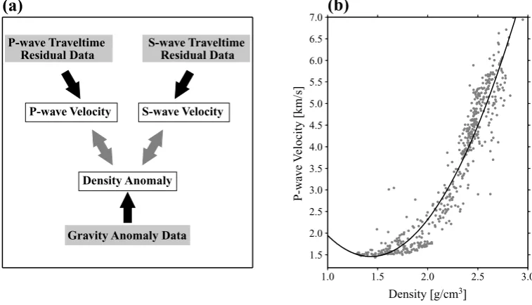
Fig. 1. (a) Basic idea of simultaneous velocity and density inversion. Heavy arrows indicate relationships between data and unknown parameters. Gray arrows show constraints between unknown parameters. In actual analysis, hypocenter locations and origin times are also determined using P- and S-wave traveltime data. In this figure, these are omitted in order to emphasize the relationships between both P- and S-wave velocities and density. (b) The relationship between P-wave velocity and density from laboratory measurements on sediments and sedimentary rocks summarized by Nafe and Drake (1963). The solid curve is the constraint between P-wave velocity and density used in the inversion.
ond purpose is to investigate the subsurface structure beneath Izu-Oshima volcano at a higher spatial resolution than was possible in previous studies. In order to obtain a high spatial resolution, we adopt the following two approaches: 1) appli-cation of a simultaneous velocity and density inversion and 2) use of traveltime data from a denser seismic network than was available to previous studies. The number of seismic stations has been increased at Izu-Oshima volcano since the latest eruption in order to better monitor the volcanic activity and to investigate subsurface structures. Currently, a seismic network composed of over 40 stations is operating and seis-mic records have been accumulated (Sakashitaet al., 1996). Densely spaced gravity measurements have also been made on the island (Andoet al., 1994).
In this paper we formulate a simultaneous velocity and density inversion using traveltime and gravity data. We then apply the method to investigate the subsurface velocity struc-ture of Izu-Oshima volcano. Finally, we discuss the impli-cations of the method and the resulting subsurface structure beneath Izu-Oshima volcano.
2.
Method
The simultaneous velocity and density inversion devel-oped in this paper obtains not only P- and S-wave veloc-ity models, but also a densveloc-ity model by using gravveloc-ity data as well as P- and S-wave traveltime data. In our inversion method the gravity data affect P- and S-wave velocities by imposing constraints between both P- and S-wave velocities and density, as shown in Fig. 1(a). The constraints between these parameters are not fixed because the relationships must have some variability. Thus, these are all unknown parame-ters.
In this study, the density structure is obtained only for the first layer because, whereas the shallower part can be well
re-solved by gravity data, it is difficult to determine the density distributions uniquely at greater depths since the distribution of gravity data is restricted to the horizontal ground surface. The constraints for the unknown parameters are also imposed at this layer. Only P- and S-wave velocities are investigated in the deeper part. In the following, the observation equa-tions and constraints required for the inversion are described and a target function is formulated.
2.1 Observation equation 1
The first observation equation is that used for the usual velocity inversion. Since traveltime data for local earth-quakes are used, hypocenter parameters and velocity param-eters must both be treated as unknowns. These paramparam-eters are determined simultaneously by
τi j= K
k=1
∂τcal i j
∂vk v
k
+ 3
l=1
∂τcal i j
∂xl
xl j+t or g
j +O(
2), (1)
where
τi j =τi jobs−τ cal i j
for P- and S-waves. τobs,τcal andτ denote the observed traveltime, the calculated traveltime and the traveltime resid-ual, respectively. v is a velocity perturbation. x and tor g are perturbations of hypocenter location and origin time, respectively. The last terms of the right-hand side in-dicate higher-orders of unknown parameters. A suffixi rep-resents a station number (i =1, . . . ,I), j an event number (j = 1, . . . ,J) andk a grid number (k = 1, . . . ,K). xl
Partial derivatives for velocity perturbations in Eq. (1) (mod-ified from Thurber (1983)) are described as
∂τcal
of m-th discrete ray segment, respectively. amk denotes a
coefficient representing weight according to distance of the
m-th discrete ray segment from thek-th velocity grid. For hypocenter locations (Lee and Stewart, 1981),
∂τcal
ds are a velocity andl-th component of ray direction
at a hypocenter, respectively.
2.2 Observation equation 2
The gravity anomalygat a point(x,y,z)due to density anomaliesρin a regionV is
g(x,y,z)= of the density anomaly inside the region V. Since in the formulation of the observation equation 1 a grid model is adopted for discrete parameterization of the unknown veloc-ity structure, the densities must also be represented at grid points. However, it is difficult to calculate the volume inte-gral in Eq. (2) analytically if the density varies continuously inside the volume. Thus, density at a grid point is represented by summation of interpolated densities of rectangular prisms smaller than the grid interval, since the gravity anomaly as-sociated with a rectangular prism having a constant density anomaly can be calculated analytically (e.g., Nagy, 1966; Talwani, 1973). The gravity anomaly at the n-th observed point due to the density anomaly of p-th rectangular prism ρpr i sm
p is
gnp=guni tnp ρ pr i sm
p .
gnpuni t indicates the gravity anomaly at the n-th observed point due to the p-th rectangular prism having unit density anomaly. This is determined by the geometric setting of the observed point and the rectangular prism. The gravity anomaly at an observation pointgn is the superposition of
density anomalies included in the regionV, thus
gn =
P
p=1
guni tnp ρpr i smp .
The density anomaly of the p-th rectangular prism is ex-pressed by a linear interpolation of density anomalies at sur-rounding gridsρkby
ρpr i sm
p =
k
bpkρk,
wherebpk is a coefficient determined by distance between
thep-th prism and thek-th grid. The right-hand side includes
eight terms relating grids surrounding thep-th prism. Hence, then-th gravity anomaly due to density anomalies at the grid points is described as
gn =
2.3 Constraints between unknown parameters
To perform the simultaneous inversion, constraints be-tween P-wave velocity and density and bebe-tween S-wave ve-locity and density are required. Empirical relations between P-wave velocity and density have been proposed based on laboratory measurements of rock samples. Birch (1961) showed, for igneous rocks, the empirical linear equation relating P-wave velocity to density, known as Birch’s law. However, this relationship is applicable to dense rocks com-monly found in deeper regions. In our inversion a relation-ship affected by porosity and appropriate for shallow struc-tures is required. Nafe and Drake (1963) plotted P-wave velocities against densities for samples of marine sediments and sedimentary rocks. Gardneret al.(1974) proposed a re-lationship for rocks from sedimentary basins. Although both studies are for porous rocks, only the former contains sam-ples having density lower than 2 g/cm3. Since the density at
depths shallower than 450 m below sea level in Izu-Oshima volcano can be lower than 2 g/cm3 (Watanabe, unpublished
data), the former relationship is more suitable. The relation-ship between P-wave velocity and density was determined by fitting a curve to the data of Nafe and Drake (1963) (see Fig. 1(b)). A polynomial expression
v(P)=a+bρ+cρ2 (4)
was selected to fit the non-linear trend and to avoid mathe-matical complexities. v(P)andρ represent P-wave velocity
and density, respectively. Constantsa,b andcwere deter-mined by least-squares resulting in a = 6.86,b = −7.55 andc=2.64.
S-wave velocity versus density of rock samples is shown by Ludwiget al.(1970). However, the number of samples is too small to determine a curve similar to that for P-wave velocity and density. Instead, the constraint between S-wave velocity and density was made through the predefined P-wave velocity and density constraint and P-P-wave velocity and S-wave velocity relationship
v(P)=αv(S), (5)
wherev(S)is S-wave velocity andαis defined for each depth.
Forα, we usedv(P)/v(S)derived from the one-dimensional
velocity inversion described later. The relationship between S-wave velocity and density can be represented as
αv(S)=a+bρ+cρ2. (6)
2.4 Target function
The observation equations and unknown parameter con-straints are combined and a target function is derived in vec-tor form. In non-linear inverse problems the following target function has been widely used to obtain unknown parame-ters:
T(m)= ||Dd(d−f(m))||2+ ||Dm(m0−m)||2, (7)
whered, m andf(m)are the data vector, model param-eter vector and a non-linear function relatingdandm, re-spectively. m0is an initial guess of model parameters. The
first term of the right-hand side is made from the observation equations and the second term is to constrain the model pa-rameters from diverging from the initial guess. Dd andDm
are diagonal matrices expressed as
Dd =
whereσd is the observational error and σm determines the
relative weight between first and second terms in Eq. (7) and corresponds to ana priorierror estimate of model parameters in the Bayesian approach (Jackson and Matsu’ura, 1985). Linear inverse problems can be regarded as special cases of the former equation and can be expressed as
f(m)=Am,
whereAis a coefficient matrix relatingdandmlinearly. In the specific case of the velocity inversion using trav-eltime data of local earthquakes, the target functionTvelcan
be constructed by replacing data vectordby observed travel-time dataτobs, model parameter vectormby P- and S-wave
velocitiesv(P),v(S), hypocenter locationxand origin time
tor g, and the non-linear functionf(m)by calculated
travel-timeτcal(v(P),v(S),x,tor g)in Eq. (7) as tively. For the density inversion, we can similarly used =
g and m = ρ = ρ−ρ0, whereg,ρ, ρ andρ0
are gravity anomaly data, density anomaly, unknown den-sity and initial denden-sity, respectively. Because the relation-ship between the gravity anomaly data and unknown density anomaly is linear, then,
Am=G(ρ−ρ0),
whereGis the coefficient matrix composed of components representing the gravity anomaly due to the unit density anomaly. The target function is
Tdens(ρ)=||Dgr ad v(g−G(ρ−ρ0))||2
+ ||Ddensm (ρ−ρ0)||2. (9)
In the simultaneous velocity and density inversion, we must combine Eqs. (8) and (9) by introducing further constraints relating the unknown parameters:
Tconst(v(P),v(S),ρ)= ||Dvcpdcvpd(v(P),ρ)||2
whereσc−1determine the weight of the constraint term.cvpd
andcvsd are constraints expressed by Eqs. (4) and (6), re-spectively. Finally, the target functionTtotal is constructed
from Eqs. (8), (9) and (10), and the unknown parameters are determined by minimizing the following function:
Ttotal(v(P),v(S),x,tor g,ρ)=Tvel(v(P),v(S),x,tor g)
+Tdens(ρ)
+Tconst(v(P),v(S),ρ). (11)
Sinceτcal,cvpd andcvsd are non-linear functions, we must
solve the problem iteratively.
3.
Application
Izu-Oshima is a volcanic island located at about 120 km SSW of Tokyo (Fig. 2(a)). It is one of the most active volca-noes in Japan, and throughout its history most eruptive ma-terials have been basaltic. Figure 2(b) shows the topography and surface features of the island. A caldera located in the center of the island is about 3 km in diameter. A central cone, Mt. Mihara, is located on the southern caldera floor. The highest elevation is 764 m above sea level. The regional stress field around the volcano is inferred as compression in the NW-SE direction and tension in the NE-SW direction from the arrangement of flank volcanoes, fissures and dikes, and from seismic focal mechanisms. The stress field is con-trolled by the collision of the Philippine Sea plate moving in a NW direction and by the bending of the plate due to sub-duction at the Sagami trough passing NE of Izu-Oshima vol-cano (Nakamuraet al., 1984). The latest eruption occurred in 1986–1987. In 1986, lava flow and pyroclastic eruptions occurred at Mt. Mihara and two newly opened fissures inside and outside the caldera. The directions of these fissures are consistent with the regional stress field.
139˚ 140˚ 34˚
35˚ 36˚
Izu-Oshima
Izu Peninsula
Tokyo
Sagami Trough
Suruga Trough
Philippine Sea Plate
(a)
Pacific Ocean Sea of Japan
139˚ 20' 139˚ 22' 139˚ 24' 139˚ 26' 139˚ 28' 34˚ 40'
34˚ 42' 34˚ 44' 34˚ 46' 34˚ 48'
139˚ 20' 139˚ 22' 139˚ 24' 139˚ 26' 139˚ 28' 34˚ 40'
34˚ 42' 34˚ 44' 34˚ 46' 34˚ 48'
Mt. Mihara
139˚ 20' 139˚ 22' 139˚ 24' 139˚ 26' 139˚ 28' 34˚ 40'
34˚ 42' 34˚ 44' 34˚ 46' 34˚ 48'
5 km
(b)
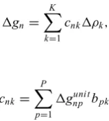
Fig. 2. (a) Index map of Izu-Oshima volcano and surroundings. The arrow indicates the direction of Philippine Sea plate motion. The enclosed area is shown in (b). (b) Topographic map of Izu-Oshima volcano showing surface volcanic features. The topographic contour interval is 50 m. The curve with tick marks indicates the caldera rim. A central cone, Mt. Mihara, rests on the southern caldera floor. Two gray lines inside and outside the caldera show locations of fissure eruption in 1986. Arrows indicate directions of principal axis of the regional stress field (Nakamuraet al., 1984). Open inverse triangles: stations equipped with a vertical component seismometer. Solid inverse triangles: stations equipped with a three-component seismometer. The numbers of stations used for the analysis were 56 for P-waves and 24 for S-waves. Crosses: locations of gravity measurement on the island. The number of gravity measurements is 447.
Makinoet al.(1988) detected an intensely magnetized body which crosses the island in a NW-SE direction, and inter-preted this body as due to solidified intrusive magma bodies.
3.1 Data
3.1.1 Arrival time data Arrival time data of local earthquakes recorded at seismic stations deployed on the volcano by Izu-Oshima Volcano Observatory, University of Tokyo (OVO) and Japan Meteorological Agency (JMA) were used for this study. In April 1986, OVO established a seismic network consisting of seven three-component seis-mometers to monitor volcanic activity. Since the 1986 erup-tion, the seismic network has been greatly expanded by OVO not only for monitoring volcanic activity, but also for inves-tigating subsurface structure. Currently, a dense seismic net-work composed of over 40 permanent stations is in operation (Sakashitaet al., 1996).
Events observed during two periods were used in our anal-ysis. These are (a) from April, 1986 through March, 1987 and (b) from August, 1995 through July, 1999. Period (a) in-cludes events that occurred during the 1986 eruption, while period (b) was non-eruptive. In period (b), hypocenters were better constrained, especially beneath the island, because of the dense seismic network. Location errors were estimated as an order of 10 m and 100–300 m for events occurred at depths less and greater than 3 km respectively at a confi-dence level of one standard deviation. Selected events for this period required that arrival times were available from many stations. However, since earthquakes occurred in re-stricted regions during the non-eruptive period, seismic rays did not sufficiently illuminate the target region. In period (a) fewer seismic stations were available than in period (b), but
hypocenters were distributed across the whole island, espe-cially for the events accompanying the eruption. For period (a), events that occurred in regions where seismicity was low in the non-eruptive period were selected.
The following conditions were imposed on the selection of seismic events. (1) Both P- and S-phases were picked. (2) For the period (a), at least seven phases were available. (3) For the period (b), at least 20 phases were available. (4) The weighted root-mean-square (WRMS) of traveltime residuals was less than 0.2 s after the initial hypocenter determina-tion. All arrival times were picked from records of 1 Hz seis-mometers. S-phases were always picked on horizontal com-ponents of seismograms from stations equipped with three-component seismometers. The number of events selected for the analysis was 504, and the numbers of stations used for P-and S-waves were 56 P-and 24 (Fig. 2(b)), respectively. The total numbers of P- and S-wave arrival times were 9675 and 2890, respectively. All of the arrival times were consistently picked for this study.
3.1.2 Bouguer anomaly data Gravity data have been obtained on the island by Andoet al.(1994) and surround-ing sea area by Katoet al.(1987). Using these data, Ando
et al. (1994) constructed a Bouguer anomaly map of the
Izu-Oshima region by assuming a Bouguer density of 2.27 g/cm3. The value was inferred from the G-H
(gravity-height) method. However, we reconstructed it by adopting the Bouguer density of 1.96 g/cm3, which was an average
Seismic Pre-Processing
Arrival Time Data
Hypocenter Location
Station Correction
Hypocenter Relocation
1-D Velocity Inversion
Gravitational Pre-Processing
Bouguer Anomaly Data
Filtering
Subtracting an Average
3-D Simultaneous Inversion
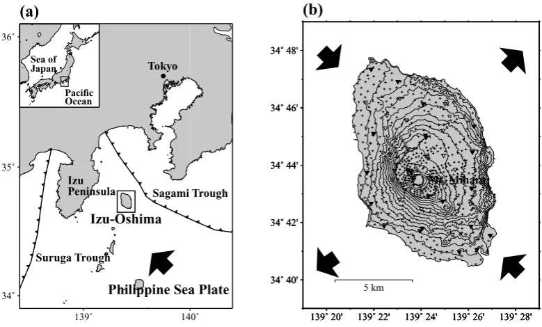
Fig. 3. Flowchart of the whole analysis. See text for explanation.
3.2 Analysis
In the simultaneous velocity and density inversion, travel-time residuals and gravity anomaly data are used. These data are constructed from arrival time and Bouguer anomaly data through the following pre-processing procedures. A flow chart of these procedures is shown in Fig. 3. Hereafter, all depths are measured from sea level.
3.2.1 Seismic pre-processing The processing of the seismic data involves (1) determining initial hypocenters, (2) determining station corrections, (3) relocating hypocenters and (4) performing a one-dimensional velocity inversion.
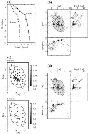
First, hypocenters for an initial one-dimensional velocity structures were determined. The one-dimensional velocity structures are shown in Fig. 4(a). Squares and circles indi-cate the depths of the grids where velocities are defined. Be-tween grids, velocities are given by linear interpolation. A grid at a depth of−1 km is set above the surface. The initial P-wave velocity structure to a depth of 2 km is based on the result of the seismic refraction experiment on Izu-Oshima is-land (Hasegawaet al., 1987). In the result of Hasegawaet al.
(1987), velocities are greater than 5.5 km/s at depths greater than 2 km. However, the WRMS of traveltime residuals af-ter the initial hypocenaf-ter deaf-terminations indicates velocities lower than 5.5 km/s are better suited for a depth of 2.5 km. After trial and error calculations, a velocity of 5.2 km/s was adopted for this depth. Velocities in regions deeper than 2.5 km are uncertain. Therefore, a profile of seismic velocity in the Izu-Bonin arc by Suyehiroet al.(1996) was referred to as representative of oceanic arc structure. Initial velocities of S-wavev(0S)were determined from initial P-wave veloci-tiesv0(P)through the relationship for a Poissonian solid, i.e., v(P)
0 /v(
S)
0 = √
3.
The locations of initial hypocenters are shown in Fig. 4(b). The occurrence of earthquakes is not uniform around Izu-Oshima volcano. Seismicity in the northwestern part is rel-atively high and events deeper than 2 km frequently occur. Depths of events inside and to the east of the caldera are almost all less than 2 km. In the southern part, fewer earth-quakes have occurred. Events located in the southeastern
part are those of seismic activity after the fissure eruption. Well-located hypocenters are preferred for the inversion. Although velocity variation exists three-dimensionally, ini-tial hypocenters were determined using the one-dimensional velocity structure. In order to remove the three-dimensional effect in shallower parts, hypocenters were relocated us-ing traveltime residuals with the station dependent correc-tions subtracted. These correccorrec-tions were made by averag-ing the traveltime residuals for each station after the initial hypocenter locations were determined. The corrected travel-time residual data were used only in the hypocenter reloca-tion step. In the steps of subsequent one-dimensional veloc-ity inversion and three-dimensional simultaneous inversion, traveltime residuals without the correction were used again because the station corrections may have included structural information, which we wanted to obtain. Figure 4(c) shows the station corrections. In general, stations with early arrivals are observed in the central part of the volcano for both P- and S-waves. This feature is consistent with the high velocity beneath the caldera revealed by former studies (Hasegawaet al., 1987; Mikada, 1994). Relocated hypocenters are much less scattered (Fig. 4(d)). This implies three-dimensional heterogeneity at shallow depths strongly affects traveltime data observed at seismic stations.
In order to obtain a better initial structure for the three-dimensional simultaneous inversion, a one-three-dimensional ve-locity inversion was performed by using traveltime residual data after the initial hypocenter determination and the relo-cated hypocenters. In this step velocities at depths from 0.25 to 6 km were treated as unknowns. Hypocenter parameters and velocities at the depths of−1 km, 8 km and deeper where rays were not sufficient were fixed to initial values. No other constraints such as damping were imposed. The result of the one-dimensional inversion is shown in Fig. 4(a).
3.2.2 Gravitational pre-processing In this study, density anomalies are investigated at only the first layer, 0.25 km. The background density at this depth was determined as 2.16 g/cm3through the P-wave velocity and density
0
Fig. 4. (a) One-dimensional velocity structure. Solid and broken lines indicate one-dimensional P- and S-wave velocity structures, respectively. Gray lines are the initial structures and heavy lines are the structures after the one-dimensional velocity inversion. Circles and squares show the depths of the grids. (b) Initial hypocentral map. Dots: initial hypocenters. 504 events were used for the analysis. (c) Station corrections for P- and S-waves. Early and delayed arrival stations are shown by darker circles with minus-symbol and lighter circles with plus-symbol, respectively. (d) Hypocenters relocated after the station corrections.
was determined fromv(P)/v(S)after the one-dimensional
ve-locity inversion.
The Bouguer anomaly data include the effect due to the density anomaly in a region from the ground surface to an unknown depth. Since in this analysis density anomalies were obtained only at the first layer, wavelengths longer than 4 km were removed from data resampled in even-space in order to remove the effect due to the density anomalies as-sociated with deeper structures. Wavelengths shorter than 1 km were also removed because the spatial interval of grav-ity measurements is approximately 500 m and components shorter than 1 km can be regarded as noise. Consequently, velocity structures whose wavelengths longer than 4 km and shorter than 1 km tend to be suppressed at the 0.25 km depth
in the resultant model.
-5
0
5
-5
0
5
-1
-1 0
0 1
2
[km]
[km]
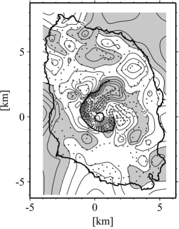
Fig. 5. Observed gravity anomaly data. Contour interval is 0.5 mgal. Shaded and white areas correspond to positive and negative anomalies, respectively.
3.2.3 Three-dimensional simultaneous velocity and density inversion After the pre-processing procedures, three-dimensional simultaneous velocity and density inver-sion was performed. Grid points in the vertical direction are the same as those in the one-dimensional velocity inversion (Fig. 4(a)). In the horizontal direction, in order to make ef-fective use of dense gravity data, we set grids at depths of −1 and 0.25 km to be finer than those in the deeper region, by modifying a method for uneven grid spacing by Yakiwara and Shimizu (1997). The intervals are 1.25 km at depths of −1 and 0.25 km, and 2.5 km at depths of 1.25 km and deeper. Grids at the depth of−1 km are set above the surface. These are for defining velocities from the surface to the depth of 0.25 km. Since rays do not penetrate at the−1 km depth, velocities are fixed to an initial value. Thus, velocities in the region shallower than 0.25 km are reflected in the result for the first layer, 0.25 km depth. Seismic rays are calcu-lated by taking into account the elevation of a seismic station. The pseudo-bending method of Um and Thurber (1987) was used to trace seismic rays in the three-dimensional inhomo-geneous medium. The local topography may affect the cal-culation of ray paths. We think, however, that the effect is not severe at Izu-Oshima volcano because the topographic vari-ation on the island is from sea level to 764 m at the summit and this range is smaller than the grid interval of the inver-sion. Thus, the topography between seismic stations is not considered. For the matrix calculation, the conjugate gradi-ent method (e.g., Scales, 1987) was used. The advantages of this method are that it requires less memory and has a quicker computation time, and the method is suitable for a large sparse matrix calculation.
In the simultaneous inversion, parameters which deter-mine the relative weight of each term in the target function (Eq. (11)) must be given. These are errors of dataσds for
P- and S-wave traveltime residuals and gravity anomalies,
parameters for terms to suppress divergence of unknowns σms for P- and S-wave velocities, hypocenter location, origin
time and density, and parameters for the constraint termσcs
between P-wave velocity and density and between S-wave velocity and density. Since the results of the inversion de-pend on these parameters, it is important to choose appro-priate values. To examine the dependencies of the inversion results on these parameters, we performed inversions using various combinations of values of parameters and compared the results. In general, these parameters affect each other. However, since the number of parameters is large in the si-multaneous inversion and it is difficult to examine all pos-sible combinations of these parameters, we performed test inversions by fixing the parameters, except for the target pa-rameter, as follows.
For σds of P- and S-wave traveltime residual data, the
picking errors of each arrival time were used. It is difficult to determine the error of each gravity anomaly data individu-ally. Therefore, based on a description by Andoet al.(1994) for errors of gravity measurements and elevation determina-tions, we adopted 0.1 mgal for error of all gravity anomaly data.
Then, we consideredσms. In general, asσms are set larger,
the data residuals are reduced, but unknown parameters tend to become divergent and may have unacceptable values. In contrast, smallerσms lead to smaller unknown perturbations
and smaller data residual reductions. Therefore, we must choose values which sufficiently reduce the data residuals and do not allow the unknowns to become divergent. Ac-cording to the result of the refraction survey (Hasegawa et al., 1987), P-wave velocities vary about 2 km/s at same depths. Thus we guess P-wave velocities can deviate about 1 km/s from the reference one-dimensional structure. In or-der to chooseσms for P-wave and S-wave velocities and
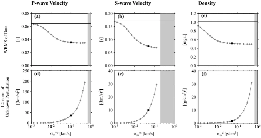
den-sity, we constructed trade-off curves of the WRMS of data versusσm(Figs. 6(a)–(c)) and of the L2-norm of model
pa-rameter perturbations from the initial value ||m0 −m||2
versus σm (Figs. 6(d)–(f)). In this step, all unknowns
ex-cept for a target parameter were fixed to initial values, and only the target parameter was dealt with as unknown. Con-straints between unknown parameters were also not consid-ered. For example, to make trade-off curves for P-wave ve-locity, we performed the velocity inversions for which the only unknown was the P-wave velocity and for which the S-wave velocity and hypocenter parameters were fixed. For the density anomaly, the test was performed by density inver-sions. It is difficult to determine the parameterσmuniquely
from the trade-off curves. We, therefore, tried several com-binations ofσms for the final inversion. Although all results
are not shown, basically similar results were obtained. The values of parameterσms selected for the simultaneous
inver-sion of which we show the results later were 0.1 km/s, 0.05 km/s and 0.05 g/cm3for P-wave, S-wave velocities and
den-sity, respectively (solid squares in Fig. 6). Then,σms for the
hypocenter locations and origin times were examined by us-ing the velocity inversion in which velocities and hypocenter parameters were unknowns. In this inversion,σms for
veloc-ities adopted in the former step were used, and 0.05 km and 0.02 s were derived.
parame-P-wave Velocity
0.00 0.02 0.04 0.06 0.08
WRMS of Data
(a)
[s]
0 50 100 150 200 250
10-3 1010-2-2 10-1 100
L2-norm of
Unkno
wn Perturbation
σmvp [km/s]
(d)
[(km/s)
2]
S-wave Velocity
0.00 0.05 0.10 0.15 0.20
(b)
[s]
0 10 20 30 40
10-3 1010-2-2 10-1 100 σmvs [km/s]
(e)
[(km/s)
2]
Density
0.0 0.2 0.4 0.6 0.8 1.0 1.2 (c)
[mg
al]
0 10 20 30 40
10-3 1010-2-2 10-1 100 σmd [g/cm3]
(f)
[(g/cm
3) 2]
Fig. 6. Trade-off curves for selecting the parameterσms. Solid squares indicate parameters selected for the inversion. Use of parameterσms within ranges
shown by hatched area leads to divergent results so large that the unknown parameters have negative value, which is physically impossible. (a)–(c): WRMS of data residuals versusσm. Solid horizontal lines indicate initial values of WRMS before the inversion. (d)–(f): L2-norm of model parameter
perturbations from the initial value||m0−m||2versusσm.
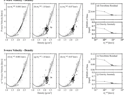
ters govern how the gravity data affect the velocity mod-els. Smaller σcs result in velocities and density for each
grid after the inversion strongly fitting the constraint curves (Figs. 7(a) and (f)), though WRMS reductions become smaller (Figs. 7(d), (e), (i) and (j)). As σcs increase,
ve-locities and density deviate from the constraint curves. Ex-tremely largeσcs lead to results similar to those of the
veloc-ity inversion and densveloc-ity inversion performed independently (Figs. 7(b) and (g) for the constraint and (d), (e), (i) and (j) for the WRMS). Our criteria for selecting appropriate val-ues were based on 1) the deviation of the samples by Nafe and Drake (1963) and 2) the WRMS of traveltime residual and gravity anomaly data. We adoptedσcs whose deviations
from the relationship after the simultaneous inversion were similar to the deviations of the samples. For the P-wave ve-locity and density constraint, we performed simultaneous in-versions where only P-wave velocity and density were un-knowns. The values ofσms determined in the previous step
were used for these unknowns. As for the S-wave velocity and density relationship, the same procedure was performed by multiplyingα, determined by the one-dimensional veloc-ity inversion, with the S-wave velocveloc-ity. Finally, 0.07 km/s was adopted for σcs of both the P-wave velocity—density
and S-wave velocity—density relationships (Figs. 7(c) and (h)). For the value ofσcs, the WRMS became as small as
those of the non-constrained case (Figs. 7(d), (e), (i) and (j)). Thus, we think the inversion result for these parameters sat-isfies both the data and the constraints.
Checkerboard tests were performed to estimate the reso-lution of the obtained structures. ±0.5 km/s anomalies were added to the reference one-dimensional velocity model for P-waves as a synthetic velocity structure. The synthetic S-wave velocity structure was constructed from the synthetic P-wave velocity through v(P)/v(S) for each grid depth determined
by the one-dimensional velocity inversion. The synthetic density anomaly structure was constructed from the P-wave velocity—density relationship and by subtracting the back-ground density from the synthetic density. Synthetic travel-time residual and gravity anomaly data were constructed for these structures. In order to represent the observational er-ror, Gaussian noise was added according to the errors of the original data. Using the synthetic data, the simultaneous in-version was performed to assess its ability to reconstruct the checkerboard velocity anomalies.
3.3 Results
The simultaneous inversion was performed using the pa-rameters determined previously, and stably converged after five iterations. Table 1 shows comparisons of values of the target functions and WRMS of data residuals before and af-ter the inversion. Reduction of the target function afaf-ter the inversion, compared to the initial value, was 72%. As for the WRMS of P- and S-wave traveltime data residuals and gravity anomaly residuals, these were 52%, 60% and 46%, respectively.
P-wave Velocity - Density
2 3 4 5 6 7
1.0 1.5 2.0 2.5 (a)σcvpd: 0.001 km/s
P-w
av
e V
elocity
[km/s]
1.0 1.5 2.0 2.5 (b)σcvpd: 1.0 km/s
Density [g/cm3]
1.0 1.5 2.0 2.5 (c)σcvpd: 0.07 km/s
0.03 0.04 0.05
[s]
(d) Traveltime Residual
0.4 0.5 0.6 0.7 0.8
10-3 1010-2-2 10-1 100
0.4 0.5 0.6 0.7 0.8
10-3 1010-2-2 10-1 100
WRMS of Data
[mgal]
σcvpd [km/s]
(e) Gravity Anomaly
S-wave Velocity - Density
2 3 4 5 6 7
1.0 1.5 2.0 2.5 (f)σcvsd: 0.001 km/s
α
* S-w
av
e
V
elocity [km/s]
1.0 1.5 2.0 2.5 (g)σcvsd: 1.0 km/s
Density [g/cm3]
1.0 1.5 2.0 2.5 (h)σcvsd: 0.07 km/s
0.06 0.08 0.10 0.12
[s]
(i) Traveltime Residual
0.4 0.5 0.6 0.7 0.8
10-3 1010-2-2 10-1 100
WRMS of Data
[mgal]
σcvsd [km/s]
(j) Gravity Anomaly
Fig. 7. (a)–(c), (f)–(h) Velocities and density after the test inversion for selectingσcs. (a) and (f) for strong constraint case. (b) and (g) for weak constraint
case. (c) and (h) for the case of parameter adopted for the inversion. Solid curve: the constraint curve used for the inversion. Gray dots: the samples by Nafe and Drake (1963). Solid circles: velocity and density values obtained after the test inversion. For the S-wave velocity—density constraint,α was multiplied with S-wave velocity to compare the samples. (d), (e), (i), (j) WRMS of traveltime residuals and gravity anomalies versusσc. Solid
horizontal lines: WRMS for the non-constrained case. Solid squares: parameters selected for the inversion.
Table 1. Target function, WRMS of data before and after the simultaneous inversion.
Target Function WRMS
P-wave [s] S-wave [s] Gra v. [mgal]
Initial 2.839×10⁵ 0.065 0.171 1.022
Final 7.341×10⁴ 0.031 0.068 0.550
(Reduction) (74 %) (52 %) (60 %) (46 %)
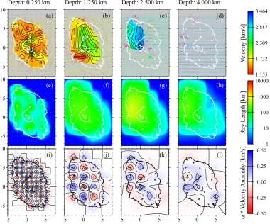
1.25 km, a high velocity belt striking in the NW-SE direction is detected. A high velocity anomaly beneath the caldera is observed at a depth of 2.5 km. At depths of 4 km and deeper, the reconstruction of the synthetic velocity structure in the checkerboard test is poor.
The synthetic S-wave model (Figs. 9(i)–(l)) is well recon-structed at 0.25 km depth, where the gravity constraint is im-posed. The pattern is still well reconstructed at 1.25 km, al-though slightly poorer than that constructed from the P-wave synthetics. At these depths, the velocity pattern is similar to the P-wave velocity model (Figs. 9(a) and (b)). At 0.25 km a high velocity region well correlated with the caldera rim is observed and coincides with the P-wave velocity model.
Little change in hypocenter locations was observed af-ter the inversion, while hypocenaf-ters obtained afaf-ter the sta-tion correcsta-tions were applied exhibited significant differ-ences from the initial hypocenters. This implies that
shal-low three-dimensional heterogeneity significantly affects the hypocenter locations.
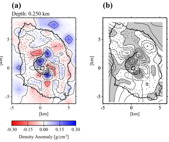
The density anomaly obtained in this inversion is shown in Fig. 10(a). The general pattern was anticipated from the observed gravity anomaly data (Fig. 5). The most prominent feature, the high density anomaly inside the caldera, was observed as expected. As seen in Table 1, the calculated gravity anomaly (Fig. 10(b)) agrees well with the observed anomaly.
4.
Discussion
4.1 Inversion method-5
Fig. 8. P-wave velocity after the simultaneous inversion using traveltime and gravity data. Light blue dots show locations of grid points. (a)–(d): resultant P-wave velocity structure. Purple dots are final hypocenters. (e)–(h): total ray length contributed for determining velocity at each grid. (i)–(l): result of corresponding checkerboard test.
-5 0 5
-5 0 5
-0.1 0 0
0
0
0
Depth: 0.250 km
[km]
[km]
-0.30 -0.15 0.00 0.15 0.30
Density Anomaly [g/cm3]
(a)
-5 0 5
-5 0 5
-5 0 5
-5 0 5
-1
-1 0
1
[km]
[km]
(b)
Fig. 10. (a) Density anomaly after the simultaneous inversion. (b) Calculated gravity anomaly. Contour interval is 0.5 mgal. Shaded and white areas correspond to positive and negative anomalies, respectively.
of 0.25 km, the pattern is almost completely reconstructed in the central part of the model. These results indicate that for P-waves, traveltime data alone are sufficient to determine the velocity structure in this grid configuration even at the first layer. Therefore, for the P-wave model, additional grav-ity data are not necessary and the increase in the amount of traveltime data results in an improved spatial resolution of the velocity structure compared to previous studies.
The synthetic S-wave checkerboard pattern was not well reconstructed at the first layer by the velocity inversion (Fig. 12), while in the simultaneous inversion the synthetic structure was reconstructed better (Fig. 9). This may indicate that the improvement in the simultaneous inversion was due to additional gravity data. However, the improvement could also be due to the contribution of P-wave traveltime data, because, in the test inversion, the synthetic S-wave velocity is consistent with not only density, but also P-wave veloc-ity through the constraint relationships, and P-wave velocveloc-ity had sufficient resolution. Thus, we performed the checker-board test for S-wave velocity and density without P-wave traveltime data in order to assess the effect by gravity data only. As a result, reconstructions very similar to those in Figs. 9(i)–(l) were obtained. Therefore we can conclude that the improvement of S-wave velocity resolution is not due to the inclusion of P-wave traveltime data. This indicates that gravity data can improve the S-wave velocity structure at the first layer where the constraint was imposed.
The area of Izu-Oshima island is about 90 km2, and the numbers of seismic stations used for this study were 56 for P-waves and 24 for S-waves. Average station intervals are about 1.3 km and 1.9 km, respectively. The station interval for P-waves is similar to the horizontal grid interval of the first layer, while for S-waves the station interval is longer. This may be a reason for the difference in the contribu-tion of gravity data to the derived velocity structure. We
also performed test inversions for P-waves which simulate sparse seismic stations and found that the results were also improved by introducing additional gravity data.
The relationship between velocity and density, and the de-viation from this relationship, are essential to this method. If the assumed relation differs from the real, incorrect results may be introduced, and improvement of the velocity struc-ture by the introduction of additional gravity data is not guar-anteed. The deviation from the relationship is also important, as it contributes to the determination of relative weights for constraints in the inversion. In this study, for P-wave velocity and density constraints, we used an empirical curve that fits data of marine sediments and sedimentary rocks (Nafe and Drake, 1963). The relationship between S-wave velocity and density was also based on this empirical curve. We selected theσcs so that the deviation after inversion was similar to that
of the rock samples used to define the curve. Currently, we do not know whether our adopted relationship and its devi-ation are the best choice for applicdevi-ation to Izu-Oshima vol-cano. At Izu-Oshima volcano, core samples were obtained from a borehole drilled in the caldera. However, the physical properties of the samples such as seismic velocities and den-sities have not yet been measured. In order to improve the results further, velocity—density relationships that are ap-propriate for the locality need to be defined. We also need to improve the theoretical framework so that it can represent not only the local relationships, but also the deviation from these relationships at the scales of inversion resolution. We will then be able to apply our method more generally.
4.2 Subsurface structure of Izu-Oshima volcano
-5
Fig. 11. P-wave velocity after the velocity inversion using traveltime data only. Notation is the same as Fig. 8. The results are similar to those shown in Fig. 8.
were obtained. The most impressive improvements are ob-served at depths of 0.25 and 1.25 km, where only a high velocity anomaly beneath the caldera had been detected in previous studies.
At the depth of 0.25 km, a high velocity area enclosed by the caldera rim was detected for P- and S-waves. This cor-relates well with the topography. This result was expected, since Andoet al.(1994) had already observed a high gravity anomaly inside the caldera rim (Fig. 5). This anomaly was interpreted as due to the accumulation of dense lava flows filling the caldera floor. In our analysis, this feature was also detected as a high velocity region.
A high P-wave velocity belt striking NW-SE direction at 1.25 km depth is newly discovered by the study. The high ve-locity region coincides with the extent of an intensely mag-netized body inferred from aeromagnetic data by Makinoet al.(1988) (Fig. 13). This anomaly can be interpreted as due to the repeated intrusion of dikes because flank volcanoes, dikes and eruptive fissures are aligned in the NW-SE direc-tion (Nakamura, 1964), which, in this region, is also the axis of maximum compressional stress into which magma is apt to intrude (Nakamura, 1977). Indeed, at the time of the fis-sure eruption in 1986, the eruptive vents trended in the NW-SE direction. Furthermore, after the beginning of the fissure eruption, hypocenters migrated to the SE and NW from the fissure vents (Yamaoka et al., 1988). From geodetic data, Hashimoto and Tada (1988) inferred that a NW-SE elon-gated tensile crack opened during the eruption. At a depth of 2.5 km, the NW-SE trending high velocity anomaly is
-5 0 5
-5 0 5
3.2 3.4 3.4
3.6
3.8
3.8 4
4.2
Depth: 1.250 km
[km]
[km]
2 3 4 5 6
Velocity [km/s]
Fig. 13. P-wave velocity at depth of 1.25 km. Area sandwiched by white lines: intensely magnetized body (Makinoet al., 1988). Purple dots: hypocenter locations of earthquakes after the fissure eruption in 1986 (Yamaokaet al., 1988). Blue line: tensile crack accompanying the eruption (Hashimoto and Tada, 1988). Red lines: the 1986 eruptive fissures.
not detected and this is perhaps due to a lower velocity con-trast between dikes and host rocks. Some dikes might have continued deeper than 2.5 km because earthquake hypocen-ters following the fissure eruption and the tensile crack in-ferred from the geodetic data extended to greater depths. At the depth of 2.5 km, a high velocity beneath the caldera was observed. In Izu-Oshima volcano, magmas have mainly erupted from the summit rather than from flank fissures, at least since the formation of the caldera about 1500 years ago, though fissure eruptions also occurred in 1986. The high ve-locity beneath the caldera may be caused by intrusive bodies related to a magmatic pathway to the summit. High veloc-ity bodies due to intruded magma have been detected along magma transport regions beneath the summit and rift zones of Hawaiian volcanoes (Okuboet al., 1997). Such intrusive bodies, which indicate magmatic pathways, were also de-tected at Izu-Oshima volcano by this study. Such prominent high velocities imply a higher proportion of intrusive rocks in these regions and that a substantial amount of magma has been emplaced under the volcano without extrusion.
The detection of a magma chamber is one of the most im-portant targets of investigations of the subsurface structure beneath volcanoes. In Izu-Oshima volcano, magma cham-bers have been inferred at depths of 4–5 km and 8–10 km by several researchers (e.g., Aramaki and Fujii, 1988; Ida, 1995;
Idaet al., 1988; Watanabe, 1990; Watanabe, 1998; Mikada
et al., 1997). In this study, however, velocity anomalies
co-inciding with these magma chambers could not be detected because few seismic rays penetrate to these depths. The tar-get region of the inversion depends on the extent of the seis-mogenic zone when we investigate velocity structure using local earthquake data. In volcanic regions, the lower limit of the seismogenic zone tends to become shallower compared to surrounding areas because of the relatively high tempera-ture of magmatic bodies (Ito, 1993). This featempera-ture can be seen in Izu-Oshima volcano (Fig. 4(d)) and prohibits our investi-gating deeper regions. For models deeper than 4 km, which are needed to clarify the magma plumbing system, use of teleseismic or regional earthquake data is required.
5.
Conclusions
We formulated a method for three-dimensional simulta-neous velocity and density inversion using local earthquake traveltime and gravity data. The gravity data contribute to P- and S-wave velocity models by imposing constraints be-tween velocities and density. For the constraints, a non-linear curve derived so as to fit the samples of porous sediments and sedimentary rocks was used. In the formulation, deviations from the constraint curve were permitted. From the results of test inversions using synthetic data, we showed that grav-ity data improves the results of the velocgrav-ity inversions at the first layer where the constraint was imposed.
rim at a depth of 0.25 km is observed, which is probably due to dense lava flows filling the caldera floor and (2) high ve-locity intrusive bodies are detected at depths of 1.25 and 2.5 km. The high velocity anomaly at a depth of 1.25 km strikes in the NW-SE direction and is interpreted as due to repeated intrusion of dikes.
Acknowledgments. We are grateful to S. Okubo, T. Iwasaki and
K. Koketsu for their helpful comments during development of this method. We are indebted to T. Kagiyama for his repeated encour-agement and constructive advice for our study. Helpful and critical comments by two reviewers, T. Ohminato and P. Dawson, greatly improved our manuscript. English usage in the manuscript was im-proved by T. Wright. We would also like to thank J. Ando, whose vigorous field work enabled us to carry out this study. For this study, we used the computer systems of Earthquake Information Center of Earthquake Research Institute, University of Tokyo.
References
Ando, J., H. Watanabe, and S. Sakashita, Study of gravity anomaly on and around Izu-Oshima volcano,Bull. Earthq. Res. Inst., Univ. Tokyo,69, 309–350, 1994 (in Japanese with English abstract).
Aramaki, S. and T. Fujii, Petrological and geological model of the 1986– 1987 eruption of Izu-Oshima volcano,Bull. Volcanol. Soc. Japan,33, S297–S306, 1988 (in Japanese with English abstract).
Birch, F., The velocity of compressional waves in rocks to 10 kilobars, part 2,J. Geophys. Res.,66, 2199–2224, 1961.
Gardner, G. H. F., L. W. Gardner, and A. R. Gregory, Formation velocity and density—The diagnostic basics for stratigraphic traps,Geophysics, 39, 770–780, 1974.
Hasegawa, I., K. Ito, K. Ono, T. Aihara, K. Kusunose, and T. Satoh, Crustal structure of Izu-Oshima island revealed by explosion seismic measurements—A profile across the island,Bull. Geol. Surv. Japan,38, 741–753, 1987 (in Japanese with English abstract).
Hashimoto, M. and T. Tada, Crustal deformations before and after the 1986 eruption of Izu-Oshima volcano,Bull. Volcanol. Soc. Japan,33, S136– S144, 1988 (in Japanese with English abstract).
Ida, Y., Magma chamber and eruptive processes at Izu-Oshima volcano, Japan: buoyancy control of magma migration,J. Volcanol. Geotherm. Res.,66, 53–67, 1995.
Ida, Y., K. Yamaoka, and H. Watanabe, Underground magmatic activities associated with the 1986 eruption of Izu-Oshima volcano,Bull. Volcanol. Soc. Japan,33, S307–S318, 1988 (in Japanese with English abstract). Ito, K., Cutoff depth of seismicity and large earthquakes near active
volca-noes in Japan,Tectonophys.,217, 11–21, 1993.
Jackson, D. D. and M. Matsu’ura, A Bayesian approach to nonlinear inver-sion,J. Geophys. Res.,90, 581–591, 1985.
Kato, S. and Seabottom Survey Group around O-Sima Volcano after 1986 Eruption, Seabottom survey around O-sima island of Izu-Ogasawara arc,
Report of Hydrographic Researches,23, 177–185, 1987 (in Japanese with English abstract).
Lee, W. H. K. and S. W. Stewart, Principles and applications of mi-croearthquake networks,Adv. Geophys. Suppl. 2, 293 pp., 1981. Lees, J. M. and J. C. VanDecar, Seismic tomography constrained by
Bouguer gravity anomalies: Applications in Western Washington, PA-GEOPH,135, 31–52, 1991.
Ludwig, W. J., J. E. Nafe, and C. L. Drake, Seismic refraction, inThe Sea, Vol. 4, edited by A. E. Maxwell, pp. 53–84, Wiley Interscience, New York, 1970.
Makino, M., T. Nakatsuka, S. Okuma, and T. Kaneko, Aeromagnetic anomalies over the Izu-Oshima volcano,Bull. Volcanol. Soc. Japan,33, S217–S223, 1988 (in Japanese with English abstract).
Mikada, H., An Elastic Scattering Theory and Its Application to the Un-derstanding of Subsurface Structure of Izu-Oshima Volcano, PhD thesis, University of Tokyo, 159 pp., 1994.
Mikada, H., H. Watanabe, and S. Sakashita, Evidence for subsurface magma bodies beneath Izu-Oshima volcano inferred from a seismic scattering analysis and possible interpretation of the magma plumbing system of 1986 eruptive activity,Phys. Earth Planet. Int.,104, 257–269, 1997. Nafe, J. E. and C. L. Drake, Physical properties of marine sediments, inThe
Sea, Vol. 3, edited by M. N. Hill, pp. 794–815, Interscience, New York, 1963.
Nagy, D., The gravitational attraction of a right rectangular prism, Geo-physics,31, 362–371, 1966.
Nakamura, K., Volcano-stratigraphic study of Oshima volcano, Izu,Bull. Earthq. Res. Inst., Univ. Tokyo,42, 649–728, 1964.
Nakamura, K., Volcanoes as possible indicators of tectonic stress orientation—Principle and proposal,J. Volcanol. Geotherm. Res.,2, 1– 16, 1977.
Nakamura, K., K. Shimazaki, and N. Yonekura, Subduction, bending and eduction. Present and Quaternary tectonics of the northern border of the Philippine Sea plate,Bull. Soc. Feol. France,26, 221–243, 1984. Okubo, P. G., H. M. Benz, and B. A. Chouet, Imaging the crustal magma
sources beneath Mauna Loa and Kilauea volcanoes, Hawaii,Geology,25, 867–870, 1997.
Sakashita, S., T. Shimomura, H. Mikada, and H. Watanabe, Volcano mon-itoring at Izu-Oshima Volcano Observatory, Earthquake Research Insti-tute, University of Tokyo,Tech. Res. Rep., Earthq. Res. Inst., Univ. of Tokyo, 7–17, 1996 (in Japanese with English abstract).
Scales, J. A., Tomographic inversion via the conjugate gradient method,
Geophysics,52, 179–185, 1987.
Suyehiro, K., N. Takahashi, Y. Ariie, Y. Yokoi, R. Hino, M. Shinohara, T. Kanazawa, N. Hirata, H. Tokuyama, and A. Taira, Continental crust, crustal underplating, and low-Q upper mantle beneath an oceanic island arc,Science,272, 390–392, 1996.
Talwani, M., Computer usage in the computation of gravity anomalies, in
Method in Computational Physics: Advances in Research and Applica-tions; Vol. 13, edited by B. A. Bolt, 473 pp., Academic Press, New York, 1973.
Thurber, C. H., Earthquake locations and three-dimensional crustal structure in the Coyote Lake Area, Central California,J. Geophys. Res.,88, 8226– 8236, 1983.
Um, J. and C. Thurber, A fast algorithm for two-point seismic ray tracing,
Bull. Seismol. Soc. Am.,77, 972–986, 1987.
Watanabe, H., Precursors to eruption and volcano prediction,Bull. Volcanol. Soc. Japan,34, S215–S226, 1990 (in Japanese).
Watanabe, H., Precursors to the 1986 eruption and the magma plumbing system of Izu-Oshima volcano,Bull. Volcanol. Soc. Japan,43, 271–282, 1998 (in Japanese with English abstract).
Watanabe, H., Borehole density data in the caldera of Izu-Oshima volcano, unpublished.
Yakiwara, H. and H. Shimizu, Three dimensional velocity structure of crust and upper mantle under the volcanoes, Kyushu,Prog. Abst. Volcanol. Soc. Japan, 1997 (in Japanese).
Yamamoto, K., Three-Dimensional P-wave Velocity Structure of Izu-Oshima Volcano, Japan by Using Teleseismic Data: for Detection of Magma Reservoir, Master’s thesis, University of Tokyo, 52 pp., 1993. Yamaoka, K., H. Watanabe, and S. Sakashita, Seismicity during the 1986
eruption of Izu-Oshima volcano,Bull. Volcanol. Soc. Japan,33, S91– S101, 1988 (in Japanese with English abstract).