Earth Planets Space,55, 395–404, 2003
A representation function for a distribution of points on the unit sphere—with
applications to analyses of the distribution of virtual geomagnetic poles
Ji-Cheng Shao1, Yozo Hamano1, Michael Bevis2, and Michael Fuller2
1Department of the Earth and Planetary Science, University of Tokyo, Japan 2HIGP/SOEST, University of Hawaii, USA
(Received November 15, 2002; Revised July 14, 2003; Accepted July 22, 2003)
An arbitrary point distribution consisting of a finite number of points on a unit sphere may be completely and uniquely represented by an analytic function in the form of a spherical harmonic expansion. The applications of this representation function are illustrated in an analysis of the symmetries in the virtual geomagnetic pole (VGP) distribution of the polarity reversal records of the past 10 million years. We find that the longitudinal confinements in the VGP distribution are (a) persistent only in the equatorially symmetric part (of the non-zonal symmetries) of the VGP distribution and (b) strong along the east coast of the North American continent and weak along the longitudes of East Asia-Australia. We also find that the equatorially symmetric patterns in the VGP distribution appear to extend preferentially into the Pacific Ocean and are relatively depleted in the longitude band associated with Africa.
Key words:Virtual geomagnetic pole, geomagnetic reversal, representation function.
1.
Introduction
The problem of analyzing the spatial distribution of a set of points on the unit sphere arises in many fields of physi-cal and natural science (Fisheret al., 1987). Frequently the points represent the orientation of vectors (e.g. arrival direc-tions) or of undirected lines (e.g. stress axes). In other cases the points represent the positions of objects or events (e.g. VGPs and earthquake epicenters). While spherical data sets of this kind can be analyzed as point distributionsper se, more typically the analyst assumes that the point set reflects or samples a population or a statistical distribution charac-terized by a continuous probability density function (PDF). In some cases, it is possible to model the point set using a standard statistical distribution, such as the Fisher, Watson or Bingham distribution (Fisheret al., 1987). These distri-butions have few parameters and fairly simple (often highly symmetric) density functions. In cases where the density of points varies in an irregular or complex fashion, and cnot be represented using standard spherical distributions, an-alysts may construct a non-parametric PDF by using numer-ical procedures. In this paper we introduce an alternative analytical function that can completely and uniquely repre-sent a point set with arbitrarily complex spatial structure on the unit sphere. We then demonstrate this function by apply-ing it to depict various symmetries in the VGP distribution and to evaluate biases in the VGP distribution of the polarity reversals of the Earth’s magnetic field for the past 10 million years.
Copy right cThe Society of Geomagnetism and Earth, Planetary and Space Sciences (SGEPSS); The Seismological Society of Japan; The Volcanological Society of Japan; The Geodetic Society of Japan; The Japanese Society for Planetary Sciences.
2.
The Representation Function for a Point
Distri-bution on the Unit Sphere
Our starting point is the Dirac delta function for a pointpˆ0 on the unit sphere,
δ(pˆ0,rˆ)= 1 4π
∞
l=0
l
m=−l
Ylm(pˆ0)Ylm(rˆ), (1)
whereYlm(rˆ)is the fully normalized surface spherical har-monic of degree l and order m, and Ym
l (rˆ) is the
com-plex conjugate ofYm
l (rˆ). The Dirac delta function satisfies δ(pˆ0,rˆ)= ∞, ifrˆ = ˆp0, andδ(pˆ0,rˆ)=0, ifrˆ = ˆp0. Next we define a functionT(L)(rˆ),
T(L)(rˆ)= 1 (L+1)2
L
l=0
l
m=−l Ym
l (pˆ0)Ylm(rˆ). (2)
Using the identity,
L
l=0
l
m=−l
Ylm(pˆ0) 2
=
L
l=0
(2l+1)=(L+1)2,
We obtainT(L)(pˆ0)=1. We then define the function
T(rˆ)= lim
L→∞T
(L)(ˆr). (3)
From (1) and (2), the function T(L)(ˆr) satisfies T(pˆ0) = 1, and T(rˆ) = 0 for every rˆ = ˆp0. T(ˆr) represents the distribution of a single point on the unit sphere. We now generalize this analysis so as to consider a finite set of points on the unit sphere. Let P = [pˆ1,pˆ2, . . . ,pˆi, . . . ,pˆK] be a
set of K distinct points on the unit sphere. We allow for coincident or duplicate points by introducing a set of point counts N = [n1,n2, . . . ,ni, . . . ,nK], where ni represents
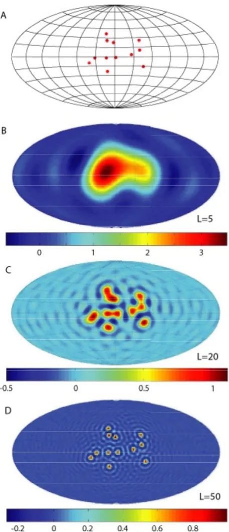
Fig. 1. A set of 12 points are located at centers of the red circles in (a). Truncated representation functions for this point set are shown in (b)–(d). They are (b)D(5)(ˆr), (c)D(20)(ˆr), and (d)D(50)(rˆ). (The colours in all maps given in this paper are linearly scaled.)
the number of points atpˆi,ni ≥ 1 for anyni ∈ N, and the
total number of points is
n=
K
i=1
ni.
We construct a distribution function for the point set P : N
by combining the distribution functions for the individual
points defined in (2). We define
D(L)(rˆ)= K
i=1
niTi(L)(ˆr).
Substituting for T(L)(rˆ)using (2), and defining the coeffi-cients,
dlm= K
i=1
J.-C. SHAOet al.: A REPRESENTATION FUNCTION FOR A DISTRIBUTION OF POINTS 397
Finally we can write the representation function for the point distributionP:N as
D(rˆ)= lim pletely represents the point distribution. The uniqueness of
D(rˆ)is obvious from Eq. (4) since for a given point set there is one and only one set of coefficientsdlm. Each of the
coeffi-cientsdlmis determined independent of the determination of
the other coefficients. Every coefficientdlmis exact, if the
po-sitions of the points are given exactly. If the popo-sitions of the points contain errors, then a mean and a variance may be as-sociated with everydlm. But there is no covariance associated
withdlm (because eachd m
l is determined independently). In
this paper, we always assume that the positions of the points are exact.
In practice, we can only use D(L)ˆrinstead of D(rˆ)to represent the point distribution. D(L)ˆris an image of the point distribution. The spatial resolution ofD(L)ˆris given by 180◦(L+0.5)which is the minimum half spatial wave-length in the spherical harmonic expansion up to degree L
(Backus et al., 1996). D(L)rˆ is, in a sense, “a blurred view (of the point distribution) obtained by a myopic ob-server who has forgotten his or her glasses” (Backuset al., 1996). The selection of a proper truncation levelL is always subjective, and there is not an ideal or even optimalLwhich may be selected in a purely objective context (perhaps, ex-ceptL = ∞). One of the useful parameters for selecting a properL is the power spectrum ofdlmdefined by,
pl =
pl is proportional to the contributions from the symmetries
of degreelto the point distribution.Lshould be chosen such thatD(L)rˆincludes the primary symmetries with largepl.
But in some cases, the analyses may require that the point distribution be approximated at different truncation levels.
Because of the finite spherical harmonic truncation, every point in the point distribution is represented by a “wavelet”
T(L)(rˆ)in (2) to approximate a unit “spike”T(ˆr)in (3). This “wavelet” is symmetrical about that point and is unit at the point. The propagations ofT(L)(rˆ)away from the point are isotropic and oscillatory in all directions with decaying mag-nitudes. Since D(L)(rˆ)is a sum of allT(L)(rˆ)on the unit sphere, it is also oscillatory. The larger positive magnitudes inD(L)(rˆ)(often significantly larger than the others while a reasonableL is chosen) are associated with the areas where the points are relatively densely populated. The magnitudes of the secondary and the high order signals in D(L)(rˆ)are often small, and can be made as small as one pleases by in-creasingL. They are usually associated with the areas where the points are relatively less populated and where no point is
distributed. The secondary and the higher order signals can be either positive or negative, corresponding to the relative magnitudes of the accretions and the depletions of the points respectively. If one wishes to analyze only the accretions of the points in the map ofD(L)(rˆ), one can then justify to sub-stitute D(L)(rˆ) = 0 for the value of D(L)(rˆ)which is less than a chosen small positive number or zero (so as to remove all negatives and some of the undesirable small positives). (Note, the negativity in D(L)rˆis not an unusual situation. For instance, any positive kernel used in geophysics, such as the Dirac delta functionδ(pˆ0,rˆ), may not always be pos-itive everywhere in the numerical computations because of the finite spherical harmonic truncation.)
We illustrate D(L)rˆby using an artificial example con-sisting of 12 points on the unit sphere as shown in Fig. 1(a). This point distribution is progressively approximated by
D(L)rˆwith L = 5, 20, 50 shown in Fig. 1(b), 1(c) and 1(d) respectively.D(50)rˆhas near zero values except at the locations near the points where it rises to nearly unit value, and is recognizably a fuzzy and approximate representation of D(rˆ). All point distributions discussed in this paper are geometrical objects. Their representation functions have no units. The colors associated with each figures are linearly scaled between the maximum and the minimum values of the representation functions respectively. The scales in Fig. 1(b), 1(c) and 1(d) may be roughly (empirically) read as the spatial distribution of the number of points in Fig. 1(a) seen in the images with spatial resolutions defined by L. For instance, when the point distribution in Fig. 1(a) is observed under the spatial resolution defined by L =15, the average num-ber of points found in the area defined by the red patch in Fig. 1(b) is roughly 3. As the spatial resolution increasing to
L =20 (this roughly means that “window size/bandwidth” decreases), average number of points found in the areas de-fined by the red patches in Fig. 1(c) is roughly little over 1. As the spatial resolution continuously increasing to in-finity (as “window size/bandwidth” decreasing to zero), the number of point found at any location equals to the number of points being distributed there—that is the representation function replicates the point distribution (in Fig. 1(a)).
One of the applications of the representation function in (6) is to separate various symmetries in a point distribution. According to (6), any point distribution on the unit sphere consists of an infinite series of geometrical symmetries de-fined by an infinite series of{dlmY
m
l (ˆr)}. These symmetries
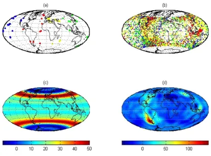
distribu-Fig. 2. Distribution of the sites and the transitional VGP (Z(15)rˆandW(15)ˆr): (a) The site distribution are divided into sectors,L1 (yellow),L2 (green),L3(blue) andL4(red) corresponding to 4 longitudinal sectors, (0, 90), (90,180), (−180,−90) and (−90, 0) respectively. (b) The distributions of the VGPs are plotted in yellow, green, blue, and red corresponding to the VGPs from the sites within the longitudinal sectorL1,L2,L3andL4 respectively (c) The zonal symmetric part of the VGP distribution in (b). (d) The non-zonal symmetric part of the VGP distribution in (b).
tion. In this paper, we first separate D(L)rˆ in terms of the zonal part Z(L)rˆ—a sum of all zonal symmetries and the non-zonal part W(L)ˆr—a sum of all non-zonal sym-metries. We then separate W(L)ˆr in terms of the equa-torial symmetriesEs(L)
ˆ
r—a sum of all terms inW(L)ˆr
satisfying l-m=even number, and the equatorial asymme-triesEa(L)
ˆ
r—a sum of all terms in W(L)rˆsatisfyingl
-m=odd number, so,
D(L)rˆ=Z(L)rˆ+W(L)rˆ
=Z(L)rˆ+Es(L)
ˆ
r+Ea(L)
ˆ
r. (8)
We shall illustrate the separations in the analyses of the VGP distribution in the following sections.
3.
The Symmetries of the VGP Distribution during
Polarity Reversal of the Earth’s Magnetic Field
Two preferential VGP paths in the polarity reversal records along the American continents and East Asia-Australia were suggested over a decade ago (Clement, 1991; Lajet al., 1991). Numerous studies on the VGP distribu-tion have been carried out since then. While the statistical significance of the preferred VGP paths has been debated in some studies (Lajet al., 1992a, b; Valetet al., 1992; McFad-denet al., 1993), the effects on the VGP distribution due to various biases and noises in the paleomagnetic data are dis-cussed in other studies (e.g. Langereiset al., 1992; Weekset al., 1992; Pr´evot and Camps, 1993; Quidelleur and Valet,
1994; Coe and Liddicoat, 1994). These debates and discus-sions continue with almost every discovery of new reversal records (e.g. Channell and Lehman, 1997). The arguments on the two preferred paths originate from various statistical tests on the VGP distribution (in which the PDF of the VGP distribution is often implicit). The tests yielded competing and sometimes conflicting results (Lajet al., 1992a, b; Valet
J.-C. SHAOet al.: A REPRESENTATION FUNCTION FOR A DISTRIBUTION OF POINTS 399
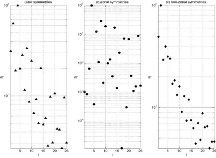
Fig. 3. The normalized power spectra for (a) the VGP distribution in Fig. 2(b), (b) the zonal symmetries in Fig. 2(c) and (c) the non-zonal symmetries in Fig. 2(d).
evaluating biases in the VGP distribution.
3.1 Representation function of the VGP distribution
Following (4), we obtain the coefficientdlm for the VGP distribution in Fig. 2(b) from,
dlm= M
j=1
Nj
i=1
¯
Ylm
ˆ
pij
, (9)
wherepˆij is theith VGP of the jth record in Fig. 2(b). The total number of the VGPs in the jth record is Nj, and the
total number of records used isM. The set of the coefficients
dlm obtained from (9) is unique. Usingdlm, we can obtain the representation function Dˆrfor VGP from (6). Dˆr
exactly replicates the VGP distribution in Fig. 2(b) as such,
Drˆ = 1 at everyrˆ = ˆpij and Drˆ = 0 elsewhere. Of course, in the numerical computations, we can only obtain
D(L)rˆfrom (5) instead of Drˆ.
In all analyses given in this paper, we chose the truncation level ofD(L)rˆatL =15. This truncation level is obtained from the normalized power spectrapl(defined in (7)) shown in Fig. 3(a) up tol =25. Clearly, the primary signals in the power spectra are from pl withl < 15. pl forl >15 tend
to be flat and many of them are less than 10% of the max-imum, implying randomness in the high order symmetries (with spatial wavelength less than 10 degrees) of the VGP distribution. Therefore, using D(15)ˆrto represent primary information in the VGP distribution (Fig. 2(b)) seems ade-quate, if not very sufficient. Truncating at lower harmonic
degrees such as L =15 is also intuitively justified because of the low expectations on the quality of the reversal data set due to, e.g. grossly inadequate site coverage on the earth’s surface and various experimental errors. Nonetheless, in or-der to be sure that the results we present in this paper are not greatly dependent on the truncation level, we actually carry out analyses at several truncation levels up to degreeL =50, and the results are consistent with those we present here.
D(15)rˆ is an image of the VGP distribution in Fig. 2(b) with spatial resolution of 10 degrees minimum half spatial wavelength. This roughly means that the figures (maps) in this paper are particularly sensitive to the signals in the VGP distribution that have a half spatial wavelength longer than 10 degrees.
3.2 Separation of the axial symmetries and the non-axial symmetries in the VGP distribution
(Fig. 2(b)) “seen” at truncation levelL =15. As L → ∞,
D(15)rˆ→ Drˆwhich replicates the VGP distribution in Fig. 2(b). Geometrically, the zonal part represents the pat-terns in the VGP distribution that are independent of the lon-gitudes and the non-zonal part represents the longitudinally dependent patterns in the VGP distribution. Obviously, this type separation facilitates the detailed analysis of a particular class of the symmetries by isolating it from the original VGP distribution (without affecting the other symmetries whatso-ever). The contributions to the VGP distribution (Fig. 2(b)) from the zonal and the non-zonal parts may be compared by using two normalized power spectra forZ(15)rˆ(computed from (7) by usingdlmwithm =0) andW(
15)ˆr(computed from (7) by usingdlm withm = 0) shown in Fig. 3(b) and
3(c) respectively.
The large signals in the zonal part (Fig. 2(c)) are concen-trated at the latitudes+/−55 degrees and are obviously due to our selection of the VGP latitudes. However, this selec-tion of the VGPs latitudes does not significantly affect the non-zonal symmetries in Fig. 2(d) because the longitudinal distribution of the VGPs at the latitudes higher than+/−55 degrees is roughly uniform with strong axial symmetries and very weak non-zonal symmetries (we verified this). Never-theless, because of the artificial restrictions of the VGP lati-tudes, all maps we present in this paper are valid only in the region between 55 and−55 degrees latitudes. The signals in the non-zonal part (Fig. 2(d)) are concentrated strongly along the longitudes of the east coast of the North American conti-nent and relatively weakly along the longitudes of East Asia-Australia. In view of the fact that the zonal part (Fig. 2(c)) is unrelated to the paleomagnetic interests concerning the lon-gitudinally dependent patterns in the VGP distribution, our analyses in this paper are only on the non-zonal part of the VGP distribution in Fig. 2(d).
3.3 Evaluation of biases in the VGP distribution
The patterns in the VGP distribution (Fig. 2(b)) and its non-zonal part (Fig. 2(d)) are contentious because of vari-ous biases in the paleomagnetic data set. For instance, in the present data set the maximum of the VGPs contributed by a reversal record is 274 and minimum is 3, with the mean and the standard deviation being 37 and 47 respectively. The number of the VGPs in a reversal record represents the num-ber of the temporal samplings of the data at the site where the reversal record is recovered. A reversal record consist-ing of large number of the VGPs is called a long reversal record, and a reversal record consisting of small number of the VGPs is called a short reversal record. Apart from a few exceptions, the majority of long reversal records are sedi-mentary records, and the majority of short reversal records are lava records. The VGP distribution (Fig. 2(b)) consists of both long and short reversal records and therefore is al-ways a biased VGP distribution. The effect of the biases is that the patterns in the VGP distribution may be greatly in-fluenced by only long reversal records, and the contributions from short reversal records are relatively reduced. Here, we propose a method using the representation function to evalu-ate biases and to estimevalu-ate the persistent patterns in the VGP distribution. We first outline the general procedures of the method. We then illustrate the method in specific examples.
3.3.1 The representation function of the weighted VGP distribution The notion of bias in a VGP distribution may be generally stated as: a group of VGPs makes far more contribution than other VGPs due entirely to some artificial factors. It follows that the evaluations of biases are to ob-serve variations of the patterns in the VGP distribution as the contributions of these dominant VGPs are reduced (or equiv-alently, the contributions from the less dominant VGPs are increased). Obviously, these evaluations are possible only if the contribution of an individual VGP to the VGP distribu-tion can be arbitrarily adjusted. In order to adjust the contri-bution of a VGP in Fig. 2(b), we modifydlmin (9) as, to the original and the removal of a VGP, pˆij respectively. Usingd˜lm, the corresponding representation function of the weighted VGP distribution denoted as D˜rˆ can then be obtained from (6). D˜rˆsatisfies,D˜ rˆ=kij for everyrˆ=
ˆ
pij, andD˜rˆ=0 elsewhere. The functionD˜rˆrepresents a set of the VGPs having the same geographic locations as those in Fig. 2(b), but a number kij is now attached to
each VGP indicating its significance. The biases in the VGP distribution can then be evaluated in the following steps:
(A) We first define a relationshipkij = F j
i [α] to adjust the
significance of a VGP,pˆijsuch thatkij of a VGP which makes a dominant contribution in the original VGP dis-tribution (e.g. the VGPs from long reversal records) is gradually reduced andkij of a VGP which makes
lit-tle contribution in the original VGP distribution (e.g. the VGPs from short reversal records) is gradually in-creased in progressive steps marked by increasing value ofα.
(B) At each step (at eachα), a set ofd˜lm(a “new VGP dis-tribution”) is obtained from (10). We denote the “new VGP distribution” as D˜(L) ric part and the equatorially asymmetric part (of the non-zonal part) of the “new VGP distribution” respec-tively. The “new VGP distribution” has the exactly the geographic distribution as the original VGP distribu-tion, but the contribution of each VGP is changed.
(C) Askijvaries (asαincreases), the biases in the VGP dis-tribution vary and are reversed (e.g. the biases in the original VGP distribution due to the dominant contribu-tions from long reversal records are gradually reversed to the biases due to the contributions from short reversal records.). The effects of biases in the original VGP dis-tribution can now be evaluated by inspecting the vari-ations in a series of maps, D˜α(L)(.), W˜α(L)(.), E˜s(αL)(.)
andE˜(L)
aα (.). The patterns that are not persistent and
J.-C. SHAOet al.: A REPRESENTATION FUNCTION FOR A DISTRIBUTION OF POINTS 401
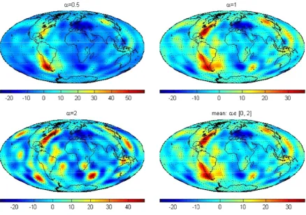
Fig. 4. The effects of biases due to uneven temporal samplings of the dataW˜α(15)rˆand the persistent patternsW¯(15)ˆrin the non-zonal part of the VGP distribution.
(D) The patterns in the maps that persist throughout the evaluations (with relatively small variations in its geo-graphic locations and amplitudes) are unlikely affected by biases. Obviously, it is not practical to display a se-ries of maps in the paper. We find that the average func-tions, denoted asW¯(L)(.), E¯s(L)(.)and E¯a(L)(.), for all maps ofW˜(L)
α (.),E˜s(αL)(.)andE˜( L)
aα (.)adequately
illus-trated (at least in the examples given in this paper) the persistent patterns “seen” during the evaluations. How-everW¯(L)(.), E¯(L)
s (.)andE¯a(L)(.)are not the “optimal
estimates” of the persistent patterns in the VGP distri-bution in any quantitative sense whatsoever.
3.3.2 Evaluating biases due to uneven temporal sam-pling of the data In this section, we evaluate biases in the VGP distribution (Fig. 2(b)) due to uneven temporal sam-pling of the data. Following step (A), we definekij as,
kij =1Njα, for α≥0, (11)
for the VGPs in jth reversal record. The relationship be-tween significance of a VGP and the length of the corre-sponding reversal record in (11) is reciprocal. As α in-creases, the contributions from long reversal records are re-duced more severely relative to those from short reversal records. For example, the significance of each VGP in a re-versal record consisting of 100 VGPs is respectively reduced to 10% forα = 1 and 1% forα = 2 relative to a VGP in a reversal record consisting of 10 VGPs. For the VGPs in the same reversal record (or in the reversal records of same
length), the significances are identical throughout the test. In the test, we useαranging from 0 to 2 in a step of 0.1. Fol-lowing step (B), we compute a set ofd˜lm up tol = 25 for each α(α = 0, 0.1, 0.2, 0.3,. . .,2) by using (10) and (11). We obtain total 21 sets ofd˜lm. We then compute W˜(15)
α
ˆ
r
from each set of d˜lm (we used˜lm withm = 0). Following step (C), we evaluate biases by inspecting a series of maps
˜
W(15)
α
ˆ
r shown in Fig. 4 for α = 0.5, 1, 2. The values in each of these maps represent the geographic variations of the non-zonal symmetric part of VGP distribution (Fig. 2(b)) with each VGP being weighted according to (11). The maps themselves represent the changes in the non-zonal symmetric part of the original VGP distribution (Fig. 2(d)), as the con-tributions from long reversal records are gradually reduced relative to the contributions from short reversal records. The changes in Fig. 4 suggest that the non-zonal part (Fig. 2(d)) of VGP distribution (Fig. 2(b)) is affected by biases due to uneven temporal samplings of the data. Following step (D), the patterns, W¯(15)rˆin Fig. 4, that are persistently seen throughout the mapsW˜α(15)ˆrare along the longitudes of the east coast of the American continents and along the lon-gitudes of East Asia. As we stated in (D),W¯(15)rˆis used only to qualitatively illustrate the persistent patterns and its relative geographic variations that we saw in a set of maps
˜
W(15)
α
ˆ
r.
Fig. 5. The persistent patterns in the VGP distribution (a)W¯(15)rˆ, (b)E¯(15)
(Fig. 2(a)). We first divide the site distribution in to four lon-gitudinal sectors. The sites within each lonlon-gitudinal sector and the VGPs contributed by the reversal records obtained at these sites are designated by the same colour as shown in Fig. 2(a) and 2(b) respectively. The total number of the VGPs contributed by the reversal records obtained within each longitudinal sector of the sites are Nv(L1) = 3092,
Nv(L2)=878, Nv(L3)=520 andNv(L4)=481 respec-tively. The differences in Nv(Li)roughly reflect both the
uneven spatial distribution of the sites and the uneven con-tributions to the VGP distribution from the reversal records obtained within different longitudinal sectors. Using the ex-actly same procedures (and the same range ofα = 0, 0.1, 0.2,. . .,2) discussed in Section 3.3.2, we first evaluate bi-ases in a VGP distribution contributed by the reversal records obtained at the sites within each of the four longitudinal sectors (the VGPs are plotted by same colour in Fig. 2(b)) due to uneven temporal samplings of the data. For each VGP distribution, we obtain 21 sets of the coefficients d˜lm
and three sets of maps W˜α(15)rˆ∈Li corresponding Nv[Li] and then summarize the functions to
obtainW˜α(15)rˆ,E˜s(α15)rˆandE˜a(15α)rˆas,
ative contributions from the longitudinal sectors containing large number of the sites and contributing large number of the VGPs. Following step (C), by inspecting a series of maps
˜
Wα(15)rˆ, E˜s(15α)rˆ and E˜a(15α)rˆ (which we do not show here), we observed that the variations in these maps are dif-ferent from those in Fig. 4. This suggests that the non-zonal part (and its equatorially symmetric and asymmetric parts) of the VGP distribution are affected by biases not only due to uneven temporal samplings of the data (discussed in Sec-tion 3.3.3) but also due to uneven spatial distribuSec-tion of the sites and the associated uneven contributions of the VGPs (the differences in Nv[Li]). Following step (D), we
illus-trate the persistent patterns seen in the maps of W˜(15)
α
in Fig. 5(a), 5(b) and 5(c) respectively.
3.4 The persistent features in the VGP distribution
One of the purposes of evaluating biases in the VGP dis-tribution is to qualitatively estimate the persistent patterns in the VGP distribution such as those shown in Fig. 5(a), 5(b) and 5(c), because these patterns likely constitute phys-ical signals of the earth’s magnetic field. In order to il-lustrate the persistent patterns in the VGP distribution con-tributed by the reversal records obtained within each of 4 longitudinal sectors respectively, we obtain persistent pat-ternsW¯(15)ˆr∈ L
for each Li obtained in Section 3.3.3. We then plot the
patches ofW¯(15)rˆ∈Li
the patches correspond to those used in Fig. 2(a) for the sites. The patches show only positive parts (the accre-tions of the VGPs) of W¯(15)ˆr∈
J.-C. SHAOet al.: A REPRESENTATION FUNCTION FOR A DISTRIBUTION OF POINTS 403
Fig. 6. The persistent patterns in the VGP distribution (a) normal to reverse polarity,E¯s(15)rˆ, (b) reverse to normal polarity,E¯(s15)rˆ, (c) the patches of
¯
Es(15)([Li])for normal to reverse polarity and (d) the patches ofE¯s(15)([Li])for reverse to normal polarity.
We also evaluated biases in the VGP distributions for the reversals from normal to reversed (N-R) polarity and from reversed to normal (R-N) polarity due to uneven spatial and temporal samplings of the data by using the same method de-scribed in Section 3.3.3, and obtained the persistent patterns in the VGP distributions for two opposite reversals. For sim-plicity, we only illustrate the persistent patterns in E¯(15)
s
ˆ
r
for N-R and for R-N in Fig. 6(a) and Fig. 6(b) respectively. The patches ofE¯s(15)rˆ∈Li
are shown in Fig. 6(c) and 6(d) respectively.
We find that the signals of large-scale concentrations per-sist in the equatorially symmetric part (of the non-zonal part) of the VGP distributions (Fig. 5(b), Fig. 6(a) and Fig. 6(b)). The strong signals broadly concentrate within two longitu-dinal confinements: one along the longitudes of the east coast of the North American continent and another (sig-nals are relatively weak and vague) along the longitudes of East Asia-Australia. The patches (Fig. 5(e), Fig. 6(c) and Fig. 6(d)) show the broadly similar longitudinal con-finements (but there are discrepancies between N-R and R-N reversals shown in Fig. 6(c) and Fig. 6(d) respectively). This suggests that the two longitudinal confinements in the VGP distributions are likely the global signals of the earth’s magnetic field during the polarity reversals. The patches in Fig. 5(e), Fig. 6(c) and 6(d) also show preferential extensions in the Pacific Ocean, but the signals in the area of preferential extensions are weaker than those in the area of the longitudi-nal confinements. Whether or not these patterns are the true signals is an interesting point to be tested by future
paleo-magnetic data. We also found that there are no large-scale systematic patterns in the equatorial asymmetries of the non-zonal part of the VGP distribution (Fig. 5(c), we do not show maps of the equatorial asymmetries for N-R and R-N rever-sals, the situations are similar to those in Fig. 5(c)). This may suggest that the equatorial asymmetries in the VGP distribu-tions are not well defined by the present data set. Whether or not there are systematic patterns in the equatorially asym-metric part of the VGP distribution should be reassessed as more data become available.
3.5 Discussion on the methods of evaluating biases in the VGP distribution
not persist, then the patterns may be artifacts. The removal of the “problematic” reversal records would of course remove biases, but at the same time it would also reduce the site cov-erage on the earth’s surface (unless of course the deleted data are nothing but noise). Therefore, if the number of the rever-sal records in the subset is far fewer than that in the original data set, then the selected subset of the data set is in fact more biased due to the inadequate and perhaps more biased distribution of the sites. Furthermore, reducing the original data set to a small subset would probably enhance other bi-ases in the subset. The removal of any data is not required in the method we discussed, but is also accommodated as an extreme case by setting the significance of a VGP to zero.
Defining the weighting factorkij in (11) is however not
unique (the weighting factors may be defined by other recip-rocal relationships). This non-uniqueness is because of the fact that we can only qualitatively define biases in the VGP distribution. If we can quantitatively define and evaluate bi-ases (of any type), it would logically mean that we could extract an “idea” or estimate an “optimal” VGP distribution (with the associated error estimates) from a biased VGP dis-tribution. We did not see how such undertakings for the pa-leomagnetic data set are logically possible. Nonetheless, in so long askij is defined following the basic requirement that
biases in the original VGP distribution are progressively re-duced (e.g. the weights of long reversal records are progres-sively reduced relative to short reversal records), we think that, logically, the outcome of these evaluations should be at least qualitatively consistent.
4.
Conclusion
The primary objective in this paper is to introduce a rep-resentation function Drˆin (6) that uniquely, completely and quantitatively represents a geometrical object—a point distribution on the unit sphere. This representation function facilitates both evaluation and manipulation of a complex point distribution analytically. There is a wealth of theorems, formulas and operators associated with spherical harmonics, and by examining spherical point distributions in terms of the infinite series of spherical harmonics, this extensive ma-chinery can be used to analyze spherical point sets. Two el-ementary applications of the representation function that we illustrate in this paper, via the analyses of the VGP distribu-tion, are (a) separating various symmetries and (b) evaluating biases in the VGP distribution.
We find that there are two persistent longitudinal confine-ments in the equatorial symmetries of the non-zonal part of the transitional VGP distribution of the polarity reversals for the past 10 million years which are similar to the two pre-ferred VGP paths suggested by other studies (Clement, 1991; Lajet al., 1991). We also find that this equatorially symmet-ric part appears to have preferential extensions in the Pacific Ocean. This implies a difference between the geometric con-figurations of the earth’s magnetic field in the Pacific
hemi-sphere and those in the hemihemi-sphere of the Prime meridian during polarity reversal. However, the signals in the areas of the extensions are weak and need to be tested by new data.
Of course, in order to systematically analyze the physical signals in the VGP distribution more relevant to the causes of paleomagntism, a better data set and a more sophisticated analytic framework is needed to deal with the issues that we have not addressed. The advanced analytic framework should include more advanced applications of the represen-tation function, the existing statistical methods and more in-put from our physical understanding of the earth’s magnetic field. We think that the representation function of a point distribution discussed in this paper is essential to the devel-opment of such a framework.
Acknowledgments. Ji-Cheng Shao wish to acknowledge a JSPS Post-doctoral fellowship from the government of Japan. We also wish to thank the editor Dr. H. Tanaka, Dr. S. Bogue and an anony-mous reviewer for their careful reviews on the manuscript and their constructive comments.
References
Backus, G., R. Parker, and C. Constable,Foundation of Geomagnetism,
Cambridge University Press, Cambridge, 158 pp., 1996.
Channell, J. E. T. and B. Lehman, The last two geomagnetic polarity rever-sals recorded in high-deposition-rate sediment drifts,Nature,389, 712– 715, 1997.
Clement, B. M., Geographical distribution of transitional VGPs: Evidence for non-zonal equatorial symmetry during the Matuyama-Brunhes geo-magnetic reversal,Earth planet. Sci. Lett.,104, 48–58, 1991.
Coe, R. S. and J. C. Liddicoat, Overprinting of natural magnetic remanence in lake sediments by a subsequent high-intensity field,Nature,367, 57– 59, 1994.
Fisher, N. I., T. Lewis, and B. J. J. Embleton,Statistical Analysis of Spheri-cal Data,Cambridge University Press, Cambridge, 329 pp., 1987. Laj, C., A. Mazaud, R. Weeks, M. Fuller, and E. Herrero-Bervera,
Geomag-netic reversal paths,Nature,351, 447, 1991.
Laj, C., A. Mazaud, R. Weeks, M. Fuller, and E. Herrero-Bervera, Geomag-netic reversal paths,Nature,359, 111–112, 1992a.
Laj, C., A. Mazaud, R. Weeks, M. Fuller, and E. Herrero-Bervera, Statistical assessment of the preferred longitudinal bands for recent geomagnetic reversal records,Geophys. Res. Lett.,19, 2003–2006, 1992b.
Langereis, C. G., A. A. M. van Hoof, and P. Rochette, Longitudinal confine-ment of geomagnetic reversal paths as a possible sediconfine-mentary artefact,
Nature,358, 226–230, 1992.
McFadden, P. L., C. E. Barton, and R. T. Merrill, Do virtual geomagnetic poles follow preferred paths during geomagnetic reversals?,Nature,361, 342–344, 1993.
Pr´evot, M. and P. Camps, Absence of preferred longitude sectors for poles from volcanic records of geomagnetic reversals,Nature,366, 53–57, 1993.
Quidelleur, X. and J.-P. Valet, Paleomagnetic records of excursions and reversals: Possible biases caused by magnetization artefacts,Phys. Earth planet. Inter.,82, 27–48, 1994.
Valet, J.-P., P. Tucholka, V. Courtillot, and L. Meynadier, Palaeomagnetic constraints on the geometry of the geomagnetic field during reversals,
Nature,356, 400–407, 1992.
![Fig. 5.The persistent patterns in the VGP distribution (a) W¯ (15) �rˆ�, (b) E¯(15s)�rˆ�, (c) E¯(15a)�rˆ�, (d) the patches of W¯ (15) ([Li]), (e) the patches ofE¯(15s)([Li]) and (f) the patches of E¯(15a)([Li]).](https://thumb-us.123doks.com/thumbv2/123dok_us/905512.1109338/8.595.85.519.73.308/fig-persistent-patterns-vgp-distribution-patches-patches-patches.webp)
![Fig. 6. The persistent patterns in the VGP distribution (a) normal to reverse polarity, E¯(15s)�rˆ�, (b) reverse to normal polarity, E¯(15s)�rˆ�, (c) the patches ofE¯(15s)([Li]) for normal to reverse polarity and (d) the patches of E¯(15s)([Li]) for reverse to normal polarity.](https://thumb-us.123doks.com/thumbv2/123dok_us/905512.1109338/9.595.75.530.74.382/persistent-patterns-distribution-polarity-polarity-polarity-reverse-polarity.webp)