Quickest Detection of a Random Signal in Background
Noise Using a Sensor Array
Taragay Oskiper
Zargis Medical Corp., Princeton, NJ 08540, USA Email:[email protected]
H. Vincent Poor
Department of Electrical Engineering, Princeton University, Princeton, NJ 08544, USA Email:[email protected]
Received 2 December 2003; Revised 21 June 2004
The problem of detecting the onset of a signal impinging at an unknown angle on a sensor array is considered. An algorithm based on parallel CUSUM tests matched to each of a set of discrete beamforming angles is proposed. Analytical approximations are developed for the mean time between false alarms, and for the detection delay of this algorithm. Simulations are included to verify the results of this analysis.
Keywords and phrases:sensor array, quickest detection, angle-of-arrival estimation.
1. INTRODUCTION
In this paper, we consider the problem of detecting, as soon as possible, a target that appears abruptly and at an unknown angle in a sensor array. This is a problem that arises in a number of applications including radar, sonar, and commu-nications. For a fixed angle of incidence and known signal and noise distributions, this is a classical problem in statis-tical change detection, and can be solved, for example, by the Page’s CUSUM algorithm. However, here we consider the situation in which the angle of incidence and the sig-nal and noise statistics are unknown. In this case, alterna-tives to the classic CUSUM must be considered, and a num-ber of such methods have been developed for such problems [1,2,3,4,5].
Here, we use an approach motivated by Nikiforov [4] in which we discretize the set of incidence angles and run parallel change-detection algorithms, each one matched to a beamformer pointed at a particular angle. The presence of a signal is announced the first time the test statistic associ-ated with any of these parallel algorithms crosses a threshold. The angle of incidence is then estimated as the pointing angle corresponding to the first test to detect. This test can be ana-lyzed by adapting the methodology of Lorden [6], and we do so by deriving expressions for the mean time between false alarms and the asymptotic mean detection delay for our test. We include a number of simulation results to verify these ex-pressions and to illustrate further properties of the proposed
algorithm, including the effects on the performance of in-creasing the number of array elements.
This paper is organized as follows. InSection 2, we de-scribe a model for the problem of interest, including rel-evant performance criteria. In Section 3, we review briefly the action and properties of the classic Page’s CUSUM test to provide a framework for our algorithm. Section 4 de-velops our parallel beamformer-based CUSUM algorithm, whileSection 5contains an analysis of the algorithm under the assumption of Gaussian noise. We also measure the per-formance of the proposed method against the optimal al-gorithm that has perfect knowledge of the signal and noise distributions together with the direction of arrival, for the case when both the signal and noise are Gaussian distributed.
Section 6discusses simulation results that illustrate the algo-rithm’s properties. And, finally,Section 7contains some con-cluding remarks.
2. STATEMENT OF THE PROBLEM
We assume a uniform linear sensor array withLelements and consider the following signal model:
yi=
ni, i=1, 2,. . .,ν−1,
a(φ)Xi+ni, i=ν,ν+ 1,. . .,
(1)
d
φ
Figure1: Linear sensor array with 5 elements with a narrowband source in the far-field impinging on the array from a directionφ.
complex-valued random signal source, is incident on the ar-ray (seeFigure 1) at an unknown angleφ∈[−π/2,π/2), and
a(φ) is theL×1 array response vector (also called the steering vector) associated with it. The array response has the follow-ing form:
a(φ)=1 e−j2π(d/λ) sin(φ) · · · e−j(L−1)2π(d/λ) sin(φ)T, (2)
whereλis the wavelength anddis the sensor spacing, typi-cally chosen as half the wavelength. Finally,{ni}is the ambi-ent noise independambi-ent of the source signal, and white in both space and time, with covariance matrixσ2
nIL.
According to the above model, before an unknown time instant ν(the change point), there is only noise in the sys-tem, and after the change point, a random signal appears at an angleφin addition to the noise. We wish to detect the ap-pearance of this random signal as soon as possible and also to estimate the angle of arrival of this source. In particular, we would like to design a detection algorithm that does not rely on the knowledge of the distribution of the random pro-cess {Xi}and the noise process{ni}, except that the noise variance is assumed to be known. In the following, we pose this problem formally as a quickest change detection prob-lem [1,6], and define the criteria involved in designing an algorithm for this purpose.
LetP(ν) denote the distribution of the sequence of
ob-servations y1,y2,. . .,yν−1,yν,yν+1,. . ., whereνis the change
point, and letE(ν)denote expectation underP(ν). We assume
that, underP(ν), the random variables{yi}are independent with a marginal probability density function (pdf) p0 for
i < νandp1 = p0fori ≥ν. LetP0correspond to the case
whereν= ∞, that is,{yi} ∼ p0for alli≥1 (the no-change
situation), and let expectation underP0 be denoted byE0.
Also, we useP1andE1 instead ofP(1)andE(1)for the case
whenν= 1, that is,{yi} ∼ p1for alli ≥ 1. The goal is to
minimize, over all possible stopping timesN, the worst-case mean delay for detection,
¯
τ(N)=sup ν≥1
ess supE(ν)
N−ν+ 1|N≥ν,y1,. . .,yν−1
,
(3)
such that the mean time before a false alarm satisfies
E0{N} ≥γ (4)
for a givenγ >0. So, the idea is to detect the presence of a change as soon as possible while keeping the false alarm rate below a desired level.
3. PAGE’S CUSUM TEST
Before moving on to the more complex case of composite hy-potheses, in the following, we review the basic case in which both the pre- and postchange hypotheses are simple. Later on, we will discretize the parameter space of the angle of ar-rival, reduce the composite alternative to a set of simple hy-potheses in that parameter, and apply parallel simple-change detection tests.
When the likelihood ratio of the observations under the two hypotheses can be written explicitly, the following algo-rithm, called Page’s CUSUM test [7], is known to be opti-mal in the minimax sense described above [6,8]. Page’s test declares the detection of a change point the first time the CUSUM statistic
max
1≤n≤iG i
n, (5)
or the equivalent and computationally efficient recursive form
Qi=
Qi−1+g
yi
+
Q0=0 (6)
exceeds a threshold h > 0, whereGi n =
i
m=ng(ym) and g(yi) = logp1(yi)/ p0(yi) is the log-likelihood function (or score function) which should satisfy 0 < ρ E1{g(yi)} <
∞. Recall that ρ = E1{g(yi)} is the Kullback-Leibler dis-tance between the two densities and is always positive, while
E0{g(yi)}is always negative.
Thus, the stopping timeNof the CUSUM algorithm is given by
N=infi≥1 : max
1≤n≤iG i n≥h
(7)
or, equivalently,
N=infi≥1 :Qi≥h
, (8)
where the equivalence is true under the condition that we use h >0. For this algorithm, we have the following well-known result of Lorden [6]:
E0{N} ≥eh, τ¯(N)=E1{N} ∼ h
ρ ash−→ ∞. (9)
Note that for the CUSUM stopping rule, the worst-case mean detection delay corresponds to the change pointν=1, since this is when the CUSUM statistic Qi ≥ 0, for alli, is at its minimum (Q0=0) and hence is the farthest from the
thresh-oldh >0.
The idea behind the CUSUM algorithm is that it stops at the first time instant i such that for some n ≤ i, the log-likelihood ratio test to decide between the hypotheses H0[i] :yn,. . .,yi∼i.i.d.p0andH(n)[i] :yn,. . .,yi∼i.i.d.p1
the recursive form (6) is that, before the change,E0{g(yi)}< 0, so thatQiremains close to zero; whereas after the change, Qistarts drifting upward with a positive meanρ=E1{g(yi)} until it ultimately crosses the thresholdh.
In general, when the likelihood ratio is not known ex-plicitly, which we assume to be so in our situation, the score functiong(·) can be replaced by any other function with neg-ative mean before the change, and positive mean after the change; that is, satisfying the conditionsE0{g(yi)} <0 and
E1{g(yi)} > 0. In this case, the stopping time is no longer guaranteed to be optimal but still a very good candidate once an appropriate function is chosen [1,9,10] satisfies
E0{N} ≥es0h, τ¯(N)=E1{N} ∼ h where s0 > 0 is the (nontrivial) root of the equation E0{esg(yi)} =1, which exists and is unique under certain
reg-ularity conditions.
4. PARALLEL BEAMFORMER-BASED CUSUM ALGORITHM
Since the angle of arrival φ after the change point is un-known, we have a composite alternative hypothesis in that parameter. Motivated by Nikiforov’s approach [4] for detect-ing a change under such a condition, we propose a simple scheme in which we run simultaneouslyKparallel CUSUM algorithms, each using a conventional beamformer. Since we assume no knowledge of the probability distributions of the target signal and noise, this suboptimal method acts as an energy detection scheme with each CUSUM “tuned” for the detection of signal energy from a particular direction of ar-rival.
The array weight vector, w(θ), for the conventional beamformer [11] (also called the fixed-phased array beam-former) is given by w(θ) = a(θ)/L, where a(θ), defined in (2), is the array response or the steering vector associ-ated with a source incident at angleθ. Hence, the output of the conventional beamformer is unity in the look direction
w(θ)Ha(θ)=(1/L)a(θ)Ha(θ)=1, wherew(θ)H is the con-jugate transpose ofw(θ). Note that the beamformer response is maximal in the look directionθ, that is,
1 weight vectorw(θ), the function
z(θ,φ)=w(θ)Ha(φ) (12)
for fixedθ, and as a function ofφ, is called thebeampattern corresponding to the beamformer pointing in the direction θ, and it is the collection of that beamformer’s responses as the angle of incidence varies overφ. On the other hand, for fixedφ,z(θ,φ), as a function ofθ, is called thesteered response corresponding to the angle of incidenceφ, and it is the collec-tion of beamformer’s responses as the look direccollec-tion varies overθ.
To devise a test for (1), we discretize the parameter space [−π/2,π/2) intoK angles{θ1,θ2,. . .,θK}such that−π/2≤ θ1<· · ·< θK < π/2. We can then design a CUSUM test for the detection of a target incident from each of such angles, operate them in parallel to provide the coverage for the whole space, and then combine them into a single change-detection algorithm. Ford=λ/2, the fixed-phased array beamformer pointing in the directionθkis defined as
wk=
The stopping time,N, of our parallel beamformer-based CUSUM test is then given by
N=infi≥1 : ¯Qi≥h
, (14)
with ¯Qidefined as follows:
¯
where we use the following equation:
gi(k)=wHkyi2−σ
2
n
L −c. (17)
Defining the functiongi(k) in the above fashion makes each CUSUM test act as an energy accumulator “tuned” to the direction θk, which will make the alarm go off in the presence of a target once it starts drifting upward collect-ing signal energy comcollect-ing from the look direction. In order to see this, first, we examine the behavior under the prechange (noise only) case. Notice that, since yi = nifori < ν, we haveE(ν){yiyiH} =σn2IL, and using the fact thatwkHwk=1/L, we obtainE(ν){gi(k)} =wkHE(ν){yiyiH}wk−σn2/L−c= −c. Here, the bias term cmust be chosen to satisfy the condi-tion c > 0, so that the expected value ofgi(k) is negative when there is no target present, that is,E(ν){gi(k)} < 0 for i < ν. This negative drift is needed to keep the CUSUM statistic Qik, 1 ≤ k ≤ K, (16) close to zero before the tar-get presence. Next, looking at the postchange behavior (sig-nal plus noise), it is easy to see that, sinceyi =a(φ)Xi+ni for i ≥ ν, and {Xi} and {ni} are independent, we have
90 60
30
0
330
300
270 0.2
0.4 0.6 0.8 1
(a)
90 60
30
0
330
300
270 0.2
0.4 0.6 0.8 1
(b)
90 60
30
0
330
300
270 0.2
0.4 0.6 0.8 1
(c)
Figure2: Beampattern samples for a two-sensor array (L=2) for look directions (a)θ=0◦, (b)θ=45◦, and (c)θ=90◦.
90 60
30
0
330
300
270 0.2
0.4 0.6 0.8 1
(a)
90 60
30
0
330
300
270 0.2
0.4 0.6 0.8 1
(b)
90 60
30
0
330
300
270 0.2
0.4 0.6 0.8 1
(c)
Figure3: Beampattern samples for a six-sensor array (L=6) for look directions (a)θ=0◦, (b)θ=45◦, and (c)θ=90◦.
is proportional to the target signal energyσ2
s, and the beam-former response for that direction |wH
ka(φ)|2, enabling the detection of the target as soon as it exceeds a certain thresh-old valueh. In particular, let the angle of arrival of the in-coming signalφ∗be such that for some ,θ =φ∗, namely, we assume that the incoming angle of arrival matches exactly one of the look directions in our set of beamformers. Then, the th CUSUM test based on that beamformer is expected to be responsible for the detection of the target since that beam-former will have the unity (and maximal) response
com-pared to the others, that is,|wHa(φ∗)| =1, forφ∗=θ. Now,
not very small compared to the difference between the beam-former look directions. Namely, for largeL, we have better resolution and, accordingly,Kmust also be chosen propor-tionately large so that we have close-to-unit response for all angles of arrivalφ. Thus, each beamformer will have an in-terval of responsibility for detection, and the union of these intervals will cover the whole region.
We can now proceed to find the mean time to a false alarm for the parallel CUSUM algorithm whose stopping time is given in (14). First, we define the followingK stop-ping times corresponding to each CUSUM rule (16):
Nkinfi≥1 :Qki ≥h
, (18)
and the final stopping time, which is equivalent to (14), is then given by
N= min
1≤k≤KN
k. (19)
Now, using the equivalent representation (7), the stopping timeNk(18) can be expressed as
Nk=minTk(n) :n=1, 2,. . ., (20)
where
Tk(n)=infi≥n:Gi n(k)≥h
(21)
withGi n(k)=
i
m=ngm(k). Hence, the stopping time (19) is given by
N= min
1≤k≤Kminn≥1T
k(n)
=min n≥1 1min≤k≤KT
k(n). (22)
For any finiten,Tk(n) is the stopping time of a sequential hypothesis test acting on observationsyn,yn+1,. . .for which
we have [1,10]
P0
Tk(n)<∞ ≤e−s0(k)h (23)
which implies
P0
min
1≤k≤KT
k(n)<∞
≤
K
k=1
e−s0(k)h, (24)
wheres0(k) is the nonzero root of the following equation:
E0
esgi(k)=1. (25)
Now, using Lorden’s theorem [6] which states that, for a stopping timeTwith respect to a sequence of random vari-ablesyi,i=1, 2,. . ., such thatP0(T < ∞)≤α, the extended
stopping timeN min{T(n)|n=1, 2,. . .}, whereT(n) is
obtained by applyingTtoyn,yn+1,. . ., satisfiesE0{N} ≥1/α,
we get from (20)–(24),
E0
Nk≥es0(k)h, (26)
and most importantly,
E0{N} ≥
1
K
k=1e−s0(k)h
. (27)
Next, based on the definition (19), the asymptotic detec-tion delay can be derived using the upper bound
E1{N} ≤ min 1≤k≤KE1
Nk (28)
together with (10), which leads to
E1{N} ∼ h
max1≤k≤KE1
gi(k)
ash−→ ∞. (29)
Finally, at the alarm timeN, as a byproduct of this al-gorithm, we can obtain an estimate of the angle of arrival, which follows from the idea that the CUSUM rule corre-sponding to the beamformer with the largest response (the one whose look direction is the closest to the angle of inci-dence) will have the sharpest increase and reach the thresh-old more quickly. Hence the estimate ˆφis obtained via
ˆ
φ=θk∗, k∗=arg max k Q
k
N. (30)
In the next section, we analyze the properties of our al-gorithm in the case where the noise in our model (1) is i.i.d. zero-mean Gaussian,ni∼N(0,σn2IL).
5. ANALYSIS UNDER GAUSSIAN NOISE
We first recall the parallel beamformer-based CUSUM test, presented in (14) with ¯QiandQki defined as before, and
gi(k)=
LwHkyi
2
σ2
n
−1−c, (31)
where it is easy to see that the thresholdhand biascvalues above are related to the ones in (14), (15), (16), and (17), by a scale factorσ2
n/L. From now on, we will use the above equiv-alent form of the CUSUM test, which makes the following analysis and interpretation of the results simpler.
Now, we look at the mean time to a false alarm for each CUSUM test in the parallel algorithm. UnderH0, that is,yi=
nifori≥1, we have
gi(k)= LwH
kni2 σ2
n
and the solution to (25) is the nonzero root of the equation
E0
es(L|wHkni|2/σn2)e−s(1+c)=1. (33) If we also assume that the real and imaginary components of the zero-mean complex Gaussian noise vectorni = ni+ jni are independent and have equal covariance, that is,
E{ninTi} =E{ninTi} = (σn2/2)IL, andE{ninTi} =
Under the assumptions made above, YR andYI are zero-mean jointly Gaussian random variables with zero covari-ance, and hence are independent, that is,
CovYR,YI =E Thus, Y is a chi-square random variable with two degrees of freedom, which is equivalent to an exponential random variable. The moment generating function ofYis then given by
EesY= 1
1−s (36)
and the solution to (25) is the nonzero root of the equation
e−s(1+c)=1−s (37)
which can be solved numerically. The solution is a function ofcand does not depend onk, so we will denote the root as
InFigure 4, we plot the nonzero roots0of the above equation
as a function of the bias termc >0. Notice that,s0approaches
1 rapidly as the biascincreases from value 0.
Next, we will look at the mean detection delay perfor-mance. Under the assumption that the incoming signal al-ways coincides with one of the look directions, that is,φ =
θ , 1≤ ≤K, the stopping time corresponding to the beam-former that is perfectly tuned to the incoming signal (the one with unit response) will beN . UnderH1, that is, when
s/σn2. Since the th beamformer’s look direction is the closest to the target, clearly we have max1≤k≤KE1{gi(k)|φ=
Now, in the case when the incoming signal is not constrained to belong to the discrete set of look directions, we will get
E1{N} ∼ h
will be close to unity, according to the preceding discussion inSection 4, provided that a sufficient number of beamform-ers K is used according to the given array sizeLsuch that for every angle of arrivalφ, the beamformer with the closest look direction has approximately unity response. Of course, this happens when the main lobes of our set of beamformers considerably overlap with each other.
Next, for the case where both the signal and noise are Gaussian, we will compare the performance of the proposed method to that of the optimal detector that has perfect knowledge of the signal and noise distributions and the an-gle of incidence. Then, as described inSection 3, the optimal CUSUM test takes the following form:
N∗=infi≥1 :Q∗i ≥h
thatρis independent of direction of arrivalφ. Hence, from (9), the mean detection delay for the optimal detector is
E1
and the lower bound on the mean time to a false alarm is given by
E0
N∗≥eh. (47)
And for the proposed parallel CUSUM method, we have
E0{N} ≥e
Now, we can investigate under what circumstances the proposed method’s performance is close to that of the opti-mal one. First, we know fromFigure 4that, as the bias term cincreases, the exponents0(c) will get closer to 1, and hence
the false alarm performance of the parallel CUSUM method
11
Figure5: Bias values for optimal mean detection delay versusσ2
s/σn2
(SNR) (cf. (50)).
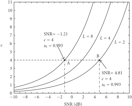
will get closer to the optimal algorithm, assuming the perfor-mance is measured with respect to the exponent term in the lower bound expression for the mean time to a false alarm. On the other hand, the detection delay performance is also related to the choice ofc, and given the antenna array size Land desired target SNR to be detected, we can determine the bias valuecin our proposed method that is needed in or-der to get the same asymptotic detection delay performance obtained from the optimal algorithm, assuming that the per-formance is measured with respect to the slope term in the asymptotic expression for the mean detection delay. So, from (41) and (46), withβ=1, we can write
from which we get
c=1 different numbers of antenna elementsL. Now, we can make the following interpretation. GivenLand SNR values, we can find the value of the bias termcthat is needed to give us mean detection delay performance equivalent to that of the opti-mal algorithm, and fromFigure 4, we can find the value of the exponents0corresponding to that bias valuec, which in
turn specifies the achievable performance on the false alarm rate given by (38). Or, givenLand the requirement on the false alarm rate determined by the value of the exponents0,
we can obtain from (37)c=(1/s) log(1/(1−s))−1, the value of the bias termcthat is needed to satisfy this requirement; and corresponding to that bias value, we can retrieve from
Given the number of sensor elementsL, we can see that the parallel CUSUM method, with c chosen according to (50), can achieve optimal detection delay performance, while its false alarm performance gets closer to the optimal as the SNR increases. For instance, looking at point B inFigure 5, we see that withL=2 and for values of SNR≥4.81 dB, we can find a bias valuec≥4, for which we get optimal detec-tion delay with false alarm performance measured in terms of the exponents0 ≥0.993, wheres0 =1 is the optimal
expo-nent. Also, looking at point A, we see that with a larger array sizeL=8, we can use the same bias valuec≥4, and achieve the optimal detection delay performance with the same false alarm performance (s0≥0.993) under lower SNR conditions
(SNR≥ −1.21 dB). So by increasing the number of antenna elementsL, we can achieve the same performance levels un-der lower SNR conditions.
Next, we will present some simulation results in order to make the ideas developed in this paper more concrete.
6. SIMULATION RESULTS
For the simulations, we will take both the noise and the in-coming signal to be i.i.d. zero-mean complex Gaussian with noise covarianceσ2
nIand signal covarianceσs2I. We choose a value of SNR =σ2
s/σn2 =5 dB, and for different array sizes L, the bias term is chosen according to (50). Overall, we per-form 10 000 Monte Carlo simulations for each data point in detection delay measurements, and 1000 Monte Carlo simu-lations for each data point in false alarm measurements. The reason why we used fewer simulations for false alarm mea-surements is that even for threshold valueshthat are much smaller than the ones we used for detection delay measure-ments, the false alarm times were much longer which made each Monte Carlo simulation take that much longer to com-plete.
In Figures2athrough3c, some sample beampatterns for a conventional beamformer with two and six sensors are plotted. We see that as the number of sensors increases, the width of the main lobe decreases and the resolution of our detector improves, which is expected to result in a better per-formance in terms of angle-of-arrival estimation. For sim-plicity, we divide the interval [−π/2,π/2) equally into 180 points and employ 180 beamformers such that each beam-formerwkpoints in the direction−π/2+((k−1)/180)π,k= 1,. . ., 180. We also note that even for 10 sensors (L = 10), where the main lobe width is very small, a separation of one degree provides the essential overlap of the main lobes of the collection of beampatterns to cover the whole region. That is to say, according to this configuration withK =180, asL ranges from 2 to 10, we getβ=0.9999 throughβ=0.9969, where we have definedβas in (42).
Now looking at Figures2athrough3c, we notice the fol-lowing. As the look direction moves away from 0◦in either direction, another sidelobe starts to appear, the beampattern starts to have asymmetry, and the peak of the second lobe increases in the opposite direction. For 90◦, there is perfect symmetry and the beamformer aimed at−90◦will have unity response for a signal coming from 90◦. For smallL, this
phe-180 160 140 120 100 80 60 40 20
20 60 100 140 180 220 260 300 340 380
E1
{
N
}
h L=2
L=4
L=8
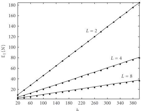
Figure6: Mean detection delay versushforL=2, 4, and 8. Solid lines: simulation; asterisks: theoretical.
nomenon is more dramatic; when we compare Figures 2b
and3b, we see that the second lobe forL=2 is much larger than it is forL=6.
We estimate the angle of arrival (30) using the idea that the beamformer whose look direction corresponds to (or is the closest to) the angle of arrival will be the one responsi-ble for the detection, since it will have the largest response among all beamformers. Ideally, we would like to have a col-lection of beampatterns in the shape of a daisy in which each petal corresponds to a specific beamformer so that we have the large responses from those beamformers that are looking in the direction of arrival, and not from those beamformers looking in the opposite direction. Now, for smallL, and for a signal coming from, say−70◦, the beamformer looking in the +70◦direction will have a significant response due to its large second lobe. Because of this, we may get large estima-tion errors coupled with a sign ambiguity. For this reason, in our simulations, we restrict the target’s angle of arrival to the interval [−50◦, 50◦] so that even forL =2, the response of the second lobe remains at a comfortably low level and we can get reliable estimates.
In the following, we investigate the properties of the al-gorithm under the case of a minimal configuration with two sensors (L=2), and we also vary the number of sensor ele-ments to observe the performance improvement achieved by increasing the array size.
200 180 160 140 120 100 80 60 40 20 0
2 3 4 5 6 7 8 9 10
L
E1
{
N
}
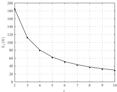
Figure7: Mean detection delay versusLforh =400. Solid line: simulation; asterisks: theoretical.
1200 1000 800 600 400 200 0
50 100 150 200 250 300 350 400 450
Co
u
n
ts
N, detection time underH1
Figure8: Histogram of detection times forh=400 andL=2.
Figure 7, where we plot the mean detection delay as a func-tion ofL, for thresholdh = 400. InFigure 8, we show the histogram of detection delays forh=400 andL=2, based on which we can make the observation that it has a gamma-like density.
InFigure 9, we plot the mean time to a false alarm for L=2, ashvaries from 1 to 6 in steps of 0.5. We see that the mean time to a false alarm increases exponentially withh. For this value ofL, we usedc=4.16 obtained from (50), and cor-responding to that, we haves0(c)=0.99. Based on this, we
can conclude that the theoretical lower bound (38) is rather loose since we gete6403, which is much smaller than the
simulation results. In Figure 10, we show the histogram of false alarm times forh= 6 andL =2, based on which we
11 10 9 8 7 6 5 4 3 2 1
1 1.5 2 2.5 3 3.5 4 4.5 5 5.5 6 h
×103
E0
{
N
}
Figure9: Simulation results for mean time to a false alarm versush
forL=2.
500 450 400 350 300 250 200 150 100 50 0
0 1 2 3 4 5 6 7 8
×104
N, false alarm time underH0
Co
u
n
ts
Figure10: Histogram of false alarm times forh=6 andL=2.
can make the observation that it has an exponential-like dis-tribution.
In Figures11and12, we look at the mean detection de-lay and the mean false-alarm time properties of the optimal detector we have defined in Section 5. ComparingFigure 6
180 160 140 120 100 80 60 40 20
20 60 100 140 180 220 260 300 340 380 h
L=2
L=4
L=8
E1
{
N
∗}
Figure11: Mean detection delay versushforL=2, 4, and 8 with the optimal algorithm. Solid lines: simulation; asterisks: theoretical.
13 12 11 10 9 8 7 6 5 4 3 2 1
1 1.5 2 2.5 3 3.5
h
×103
E0
{
N
∗}
Figure12: Simulation results for mean time to a false alarm versus
hforL=2, with the optimal algorithm.
detection delay as a function of thresholdhfor different array sizesL=2, 4, and 8. We see the standard deviation increases withhand the gap between the optimal and the proposed method is smaller for largerL.
In Figure 14, we consider the mean-squared angle-of-arrival estimation error as a function of thresholdh, while keeping the number of sensors fixed (L=2). As we increase h(causing more delay in detection), initially we see consid-erable improvement which diminishes slowly as we further increase the threshold size. InFigure 15, we again look at the mean-squared estimation error; this time with a larger ar-ray size (L = 6), and see that the estimation errors are sig-nificantly lower. In Figure 16, we vary the number of sen-sors in the array for a fixed detection threshold h = 20,
45 40 35 30 25 20 15 10 5
20 60 100 140 180 220 260 300 340 380 h
L=2
L=4 L=2
L=8
L=4 L=8
Standar
d
de
vi
ation
o
f
d
et
ection
dela
y
Figure13: Simulation results for the standard deviation of the de-tection delay times versushforL=2, 4, and 8. Solid lines: parallel CUSUM method; dashed lines: optimal algorithm.
26 24 22 20 18 16 14 12 10 8 6 4 2
20 60 100 140 180 220 260 300 340 380 h
E1
{
(
ˆφ−
φ
)
2}
Figure14: Mean-squared angle-of-arrival estimation error versus
hforL=2.
and observe that the mean-squared error exhibits a sharp decrease initially asLincreases from 2, and then tapers off. Note that while comparing the estimation errors as a func-tion ofLfor a fixed thresholdh, we should keep in mind that we not only get a reduction in the mean-squared estimation error with a larger array size, but also we detect the target sooner as evident from Figures 6 and7. Finally, Figure 17
shows the histogram of squared estimation error forh=100 andL=6.
7. CONCLUSION
1.6 1.4 1.2 1 0.8 0.6 0.4 0.2
20 60 100 140 180 220 260 300 340 380 h
E1
{
(
ˆφ−
φ
)
2}
Figure15: Mean-squared angle-of-arrival estimation error versus
hforL=6.
28 26 24 22 20 18 16 14 12 10 8 6 4 2 0
2 3 4 5 6 7 8 9 10
L
E1
{
(
ˆφ−
φ
)
2}
Figure16: Mean-squared angle-of-arrival estimation error versus
Lforh=20.
we have applied a sensor array and devised a parallel CUSUM algorithm based on beamforming. The algorithm not only detects quickly the existence of the target, but it also provides an estimate on the target’s angular direc-tion. We have developed analytical bounds on the algo-rithm performance and verified these bounds through sim-ulation, and also demonstrated the algorithm’s eff ective-ness by varying different parameters in the system. We have also compared, under the Gaussian signal and noise case, the proposed algorithm’s performance against the op-timal algorithm that has perfect knowledge of the sig-nal and noise distributions, together with the direction of arrival.
6 5 4 3 2 1 0
×103
0 1 2 3 4 5 6 7
Co
u
n
ts
Angle-of-arrival estimation error|φˆ−φ|
Figure17: Histogram of angle-of-arrival estimation error forL=6 andh=100.
ACKNOWLEDGMENT
This research was supported by the US Office of Naval Re-search under Grant no. N00014-03-1-0102.
REFERENCES
[1] M. Basseville and I. V. Nikiforov,Detection of Abrupt Changes: Theory and Application, Prentice Hall, Englewood Cliffs, NJ, USA, 1993.
[2] G. Lorden, “Nearly-optimal sequential tests for finitely many parameter values,” Annals of Statistics, vol. 5, no. 1, pp. 1–21, 1977.
[3] I. V. Nikiforov, “A generalized change detection problem,”
IEEE Transactions on Information Theory, vol. 41, no. 1, pp. 171–187, 1995.
[4] I. V. Nikiforov, “A suboptimal quadratic change detection scheme,” IEEE Transactions on Information Theory, vol. 46, no. 6, pp. 2095–2107, 2000.
[5] T. Oskiper and H. V. Poor, “Online activity detection in a multiuser environment using the matrix CUSUM algorithm,”
IEEE Transactions on Information Theory, vol. 48, no. 2, pp. 477–493, 2002.
[6] G. Lorden, “Procedures for reacting to a change in distri-bution,” Annals of Mathematical Statistics, vol. 42, no. 6, pp. 1897–1908, 1971.
[7] E. S. Page, “Continuous inspection schemes,”Biometrika, vol. 41, no. 2, pp. 100–115, 1954.
[8] G. Moustakides, “Optimal procedures for detecting changes in distributions,” Annals of Statistics, vol. 14, pp. 1379–1387, 1986.
[9] B. Broder, Quickest detection procedures and transient signal detection, Ph.D. dissertation, Department of Electrical Engi-neering, Princeton University, Princeton, NJ, USA, 1990. [10] B. K. Ghosh, Sequential Tests of Statistical Hypotheses,
Addison-Wesley, Reading, Mass, USA, 1970.
Taragay Oskiper was born in Ankara, Turkey, in 1974. He received the B.S. de-gree in electrical engineering from Bilkent University, Ankara, Turkey, in 1996, and the M.S. and Ph.D. degrees in electrical engi-neering from Princeton University, Prince-ton, NJ, in 1998 and 2001, respectively. His research interests are in the areas of statis-tical signal processing, theory of detection and estimation, and wireless
communica-tions. Since 2001, Dr. Oskiper’s employment has been with Zargis Medical Corp., where he is developing advanced signal processing algorithms for computer-aided analysis of heart sounds.
H. Vincent Poorreceived the Ph.D. degree in electrical engineering and computer sci-ence from Princeton University in 1977. From 1977 till 1990, he was on the fac-ulty of the University of Illinois at Urbana-Champaign. Since 1990, he has been on the faculty at Princeton University, where he is the George Van Ness Lothrop Professor in engineering. Dr. Poor’s research interests are in the areas of wireless networks,