Polar motion prediction using the combination of SSA and Copula based analysis

FULL PAPER

Polar motion prediction using

the combination of SSA and Copula-based

analysis

Sadegh Modiri

_{, Santiago Belda}

_{, Robert Heinkelmann}

_{, Mostafa Hoseini}

_{, José M. Ferrándiz}

and Harald Schuh

Abstract

The real-time estimation of polar motion (PM) is needed for the navigation of Earth satellite and interplanetary space-craft. However, it is impossible to have real-time information due to the complexity of the measurement model and data processing. Various prediction methods have been developed. However, the accuracy of PM prediction is still not satisfactory even for a few days in the future. Therefore, new techniques or a combination of the existing methods need to be investigated for improving the accuracy of the predicted PM. There is a well-introduced method called Copula, and we want to combine it with singular spectrum analysis (SSA) method for PM prediction. In this study, first, we model the predominant trend of PM time series using SSA. Then, the difference between PM time series and its SSA estimation is modeled using Copula-based analysis. Multiple sets of PM predictions which range between 1 and 365 days have been performed based on an IERS 08 C04 time series to assess the capability of our hybrid model. Our results illustrate that the proposed method can efficiently predict PM. The improvement in PM prediction accuracy up to 365 days in the future is found to be around 40% on average and up to 65 and 46% in terms of success rate for the PMx and PMy , respectively.

Keywords: Copula, SSA, Polar motion, EOP, Prediction

© The Author(s) 2018. This article is distributed under the terms of the Creative Commons Attribution 4.0 International License (http://creat iveco mmons .org/licen ses/by/4.0/), which permits unrestricted use, distribution, and reproduction in any medium, provided you give appropriate credit to the original author(s) and the source, provide a link to the Creative Commons license, and indicate if changes were made.

Introduction

Polar motion (PM) describes the movement of the Earth’s rotation axis w.r.t the Earth surface. The study of PM pro-vides valuable information for studying many geophysical and meteorological phenomena (Barnes et al. 1983; Wahr

1982, 1983; Mathews et al. 1991; Gross et al. 2003; Chen and Wilson 2005; Gross 2015; Seitz and Schuh 2010; Schuh and Böhm 2011).

Since the 1960s, highly accurate PM coordinates can be obtained by different space geodesy techniques. These techniques include: Satellite Laser Ranging (SLR) (Cou-lot et al. 2010), Lunar Laser Ranging (LLR) (Dickey et al.

1985), Doppler Orbitography and Radiopositioning Inte-grated by Satellite (DORIS) (Angermann et  al. 2010), Global Navigation Satellite Systems (GNSS) (Dow et  al.

2009; Byram and Hackman 2012), and very-long-baseline interferometry (VLBI) (Schuh and Schmitz-Hübsch 2000; Nilsson et al. 2010, 2011, 2014).

Accurate real-time PM is needed for high-precision satellite navigation and positioning and spacecraft track-ing (Kalarus et al. 2010; Stamatakos 2017). However, the PM is not provided in real time due to the complexity of the measurement model and data processing; PM coordi-nates are available with a delay of hours to days (Bizouard and Gambis 2009; Schuh and Behrend 2012). Therefore, it is essential to predict the PM parameters precisely.

Different methods and means have been investigated and applied for PM prediction such as least squares (LS) colloca-tion (Włodzimierz 1990), spectral analysis and LS extrapo-lation method (Akulenko et al. 2002), LS extrapolation of a harmonic model and autoregressive (AR) prediction (Kosek et al. 1998, 2007; Xu et al. 2012), wavelets and fuzzy infer-ence systems (Akyilmaz and Kutterer 2004; Akyilmaz et  al. 2011) modeling and forecasting excitation functions

Open Access

*Correspondence: [email protected]

1 _{GFZ German Research Centre for Geosciences, Potsdam, Germany}

(Chin et al. 2004), Kalman filter with atmospheric angular momentum forecasts (Freedman et  al. 1994), and artifi-cial neural network (ANN) (Schuh et al. 2002; Kalarus and Kosek 2004). The Earth orientation parameters prediction comparison campaign (EOP PCC) took place within (2005– 2009), and the results demonstrate that there is no particular method superior to other for all prediction intervals (Kala-rus et  al. 2010). Among these methods, the combination of LS and AR process is considered to be one of the most effective for PM prediction (Kalarus et al. 2010). The men-tioned combination method achieved reasonable results for short-term forecasting. However, due to the complexity of the PM excitation model, it is not able to reproduce the time variation of the periodic terms that influence the long-term predictive accuracy of PM. Consequently, a new prediction method is required that could bring us significantly closer to meeting the accuracy goals pursued by the Global Geo-detic Observing System (GGOS) of the International Asso-ciation of Geodesy (IAG), i.e., 1 mm accuracy and 0.1 mm/ year stability on global scales in terms of the ITRF defining parameters (Plag and Pearlman 2009). Therefore new tech-niques or a combination of the existing methods need to be investigated for improving the efficiency of the predicted PM considering the time variation of the periodic terms and the trend. In this study, we examined the combination of singular spectrum analysis (SSA) and Copula-based analy-sis to predict PM. SSA is not constrained by the assump-tions of using predetermined funcassump-tions such as sine wave as the base; it rather exploits data-driven base functions for extracting fundamental components of the time series and applies a classification method to explore the relationship between the derived elements (Broomhead and King 1986; Vautard et al. 1992; Zotov 2005). The Copula method oper-ates linear and nonlinear dependency between variables, and it is a potent and efficient tool for dealing with multi-dimensional data and modeling the relationship between parameters (Joe 1997). The combination of SSA and Cop-ula-based methods will be applied for the first time as a novel stochastic tool for PM determination.

PM is the sum of two statistically independent parts: trend and undulation. This hybrid model consists of a deterministic annual and the Chandler component as well as long-term lower-frequency parts which are estimated by SSA. The difference between the deterministic solution and the PM data is then used in a Copula-based model to pre-dict stochastic processes. Then, the final PM prepre-diction is a combination of the deterministic prediction (derived from the SSA solution) and the stochastic prediction (obtained from the Copula solution). To this end, first, the time series of PM from EOP 08 C04 were analyzed, and the trend is modeled and separated by SSA. Then, a Copula prediction model is made based on the SSA-separated time series.

Finally, the accuracy of the proposed combined method is verified through different sets of PM prediction tests.

Methodology

In this study, we developed and explored the integration of Copula-based analysis and SSA for precisely predicting PM.

Singular spectrum analysis

To maximize the prediction performance, we need a mathematical tool to retrieve all time-correlated infor-mation from the time series. As a matter of fact, the existence of excitations of PM can profoundly affect the forecasting procedure, particularly in longer intervals. Therefore, the exploitation of efficient techniques is cru-cial to minimize the risk of having gross errors.

SSA is a nonparametric spectral estimation method which can be used for decomposing a time series into the sum of interpretable components, e.g., trend, periodic components, and noise, without a priori assumption about the constituent components (Golyandina et al. 2001).

SSA is able to remove redundancies and groups uncor-related information into informative empirical functions which can reveal main aspects of the time series. The mentioned functions are used as bases of a subspace in which the time series is a member of and can be exploited for modeling the time series in a desired level of details. Therefore, the model can simulate the future entries of the time series using these base functions.

The SSA method for trend extraction can be succinctly expressed as two stages:

Decomposition First the time series is embedded in an L-dimensional vector space. The outcome of this stage will be a trajectory matrix ( X ) which consists of L rows.

being 1<L<K and K =N−L+1.

Having the trajectory matrix formed, singular value decomposition (SVD) is applied to factorize X in the

form of UVT in order to retrieve its principal

compo-nents (PC).

where U and V are the left and right singular vectors,

respectively, and is a diagonal matrix consisting of

sin-gular values of X which reflect the importance of each

corresponding pair of left–right singular vectors. The decomposition step can be performed using calculation of eigenvalues and eigenvectors of the matrix S=XXT.

Let ₁≥₂≥ · · · ≥_L≥0 denote diagonal entries of

(the eigenvalues of S ) and _U1,U2,. . .,UL indicate the

cor-responding eigenvectors of S which are also called empir-ical orthogonal functions (EOF) of X . The right singular

vectors of X are eigenvectors of XTX calculated by:

Now, the trajectory matrix can be written as:

Reconstruction This stage aims to rebuild the time series using the reconstructed version of trajectory matrix. So, a subset of A= {X_{1, X2,}. . ., Xd} can be chosen for recon-struction of the trajectory matrix. The choice of PCs of X

defines how smooth would be the reconstructed version of the time series and how much detail of the original time series would be captured. Having a proper selection of PCs, a representative trend is extracted by applying diagonal averaging to the reconstructed trajectory matrix ( Xˆ) . Let L<K , and then, the trend of the time series

There is a well-introduced method called Copula that can be applied for polar motion modeling, estimation, and prediction. The word of Copula is a Latin noun that means a link or tie. The Copula method exploits linear and non-linear dependency between variables. It is a potent and efficient tool for dealing with multi-dimensional data and modeling the relation between parameters based on the marginal distribution functions of the variables (Embre-chts et al. 2002). Copula appeared in the context for the first time by Sklar (1959). Sklar’s theorem indicates that a Copula function C connects a given multivariate distribu-tion funcdistribu-tion with its univariate marginal. For bivariate distribution, there is a bivariate Copula C which models the joint cumulative probability distribution function of two variables X and Y based on the marginal cumulative distribution functions FX(x) and FY(y).

where C describes the joint distribution function FX,Y(x,y).u and v are transformed of X and Y to uniform

distribution, respectively. Then, Joe (1997) and Nelsen (2007) developed the idea of the Copula. For many years, the Copula method has been used for modeling the dependence structure between random variables in different types of studies, e.g., economics (Rachev and Mittnik 2000; Patton 2006, 2009), biomedicine (Wang and Wells 2000; Escarela and Carriere 2003), hydrology (Bárdossy and Li 2008; Bárdossy and Pegram 2009; Ver-hoest et  al. 2015), meteorology (Laux et  al. 2011; Vogl et al. 2012), hydro-geodesy (Modiri et al. 2015). A brief introduction to the concept of copula function is given in the next subsections.

Characteristic of Copulas

In the bivariate case, a Copula is represented as a func-tion C from [0, 1]2 _{to [0, 1] so that ∀u,v∈ [0, 1] (Genest}

and Rivest 1993; Jaworski et al. 2010):

Copula is a continuous function:

The Copula density is computed by differentiating Cop-ula cumCop-ulative distribution function.

Empirical Copula

The empirical Copula is an estimator for the unknown theoretical Copula distribution, and it is defined in the rank space as follows (Genest and Rivest 1993; Genest and Favre 2007; Laux et al. 2011):

n is the length of the data vector,

1_{(...) is the indicator function. If the condition is}

true, the indicator function is equal to 1. Otherwise, the indicator function is equal to 0.

Archimedean Copula

A number of Copulas can be estimated directly with the simple form. They are named Archimedean Copulas. An Archimedean Copula can be presented in the following form:

where θ is the Copula parameter and the function φ is the generator of the Copula with the following characteristics (Nelsen 2007):

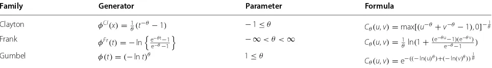
There are three commonly used Archimedean Copula which are explained as follows and will be investigated in this study (see Table 1).

(1) Clayton Copulas

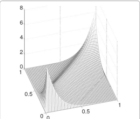
The generator of the Clayton Copula (see Fig. 1) is given by

Therefore, the cumulative distribution function (CDF) for Clayton Copula is defined as (Clayton 1978):

an asymmetric Archimedean Copula; it shows greater dependence in the lower tail than in the upper tail

Table 1 Three ordinary families of  Archimedean Copulas (Clayton, Frank, and  Gumbel Copula) and  their generator, parameter space, and their formula

θ is the parameter of the Copula called the dependence parameter, which measures the dependence between the marginal

where θ is restricted on the interval [−1,∞) . If

θ =0 , it shows the independence case and when

θ → ∞ , indicate high dependency in the lower

rank space.

(2) Frank Copula

The generator of the Frank Copula (see Fig. 2) is given by

The parameter θ is defined over ∈(−∞,∞)− {0} . The CDF for Frank Copula is given by (Joe 1997; Lee and Long 2009)

Frank Copula allows to model data with positive and negative dependency. The large positive and negative θ indicate high dependency, and θ =1 implies total independence. The Frank Copula is a suitable method for two data sets with the same dynamic characteristics (Rodriguez 2007).

(3) Gumbel Copulas

Gumbel Copula (see Fig. 3) is famous for its ability to capture strong upper tail dependence and weak lower tail dependence. Gumbel Copula is used to model asymmetric relationship in the data

(Jawor-(18)

φFr(t)= −ln

e−θt−1 e−θ₋₁

(19) Cθ(u,v)=

1

θ ln

1+ (e

−θu_−1)(e−θv₎

e−θ₋₁

ski et  al. 2010). The Gumbel Copula generator is written as:

The CDF for Gumbel Copula is given by (Nelsen 2007)

The Copula parameter θ is on the interval [1,+∞) . If θ is equal 1, Copula shows independence. When θ → ∞ , the Gumbel Copula indicates high depend-ence between the random variables.

Copula parameter estimation

The widely used estimation method for the Copula parameter is the maximum likelihood (ML) estima-tion methodology (Joe 1997). The Copula parameters in this study are derived from ML estimation. The canoni-cal maximum likelihood estimation (CLME) and infer-ence for margins estimation (IFME) are two methods for estimation of the Copula parameter (Joe and Xu 1996). For both methods, the first step is marginal distribution estimation. Then, a pseudo-sample of the transformed observation is used to estimate the Copula parameter. In the IFME method, the theoretical marginal distribution parameters are estimated, and in the CMLE the univari-ate marginals are the empirical distribution functions (Giacomini et al. 2009). It is assumed that the sample data (X1,X2,X3,. . .,Xn) are n independent and identically

(20)

φ (t)Gu=(−lnt)θ

(21) Cθ(u,v)=e−((−ln(u)

θ_)+(−ln(v)θ₎₎1θ

Fig. 2 Frank Copula with parameter θ=8 . The Frank Copula is a

symmetric Archimedean Copula

Fig. 3 Gumbel Copula with parameter θ=3 . Gumbel Copula

distributed (iid) random variables. These data are trans-formed into uniform variates (r1,r2,r3,. . .,rn).

Let c(r1,r2,r3,. . .,rn) be the density function of Copula

C(r1,r2,r3,. . .,rn;θ ) , and let θ be the Copula parameter which is estimated by maximizing the ML equation:

Computation of conditional CDF for Archimedean Copula In this subsection, the conditional CDF of Clayton, Frank, and Gumbel Copula are computed (Yue 1999; Zhang and Singh 2007; Trivedi et al. 2007). The conditional CDF for Clayton Copula is given by (Joe 1997):

and for Frank Copula:

The conditional CDF of Gumbel Copula is:

Simulating from Copula‑based conditional random data This subsection provides the essential steps for data sim-ulation using Copula-based conditional random data. The following steps are taken to fit the suitable theo-retical Copula function and simulation data (Laux et al.

2011; Vogl et al. 2012).

(1) Independent identical distribution (iid)-transfor-mation of input time series.

(2) Compute the marginal distribution FX(x) and FY(y) of the input data x and y.

(3) Transform data to rank space using the estimated marginal distributions of data with ui and vi in rank space.

(4) Compute the empirical Copula to the dependence structure of random variables using the rank-trans-formed data.

(5) Fit a theoretical Copula function Cθ(u,v). (6) Compute the conditional Copula function.

(7) Sample random data from the conditional Copula CDF.

(8) Transfer the sample back to the data space using the inverse marginal.

Error analysis

The mean absolute error (MAE) standard is used in order to evaluate the prediction accuracy. It can be shown as follows:

where Pi is the predicted value of the i-th prediction, Oi is the corresponding observation value, Ei is the error, and n is the total prediction number (Willmott and Matsuura

2005).

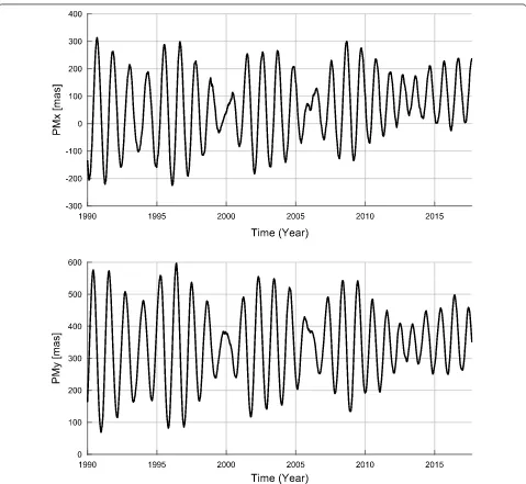
Calculation and analysis Data description

In this paper, the PMx and PMy time series (see Fig. 4) are from the International Earth Rotation and Reference Sys-tems Service (IERS) combined earth orientation param-eter (EOP) solutions 08 C04 (available at http://hpier s.obspm .fr/eop-pc/analy sis/excit activ e.html). The EOP 08 C04 series is derived from different geodetic tech-niques, and it is consistent with ITRF 2008. The EOP 08 C04 time series cover the period 1962 to the present. The sampling interval is one day.

Data processing and analysis

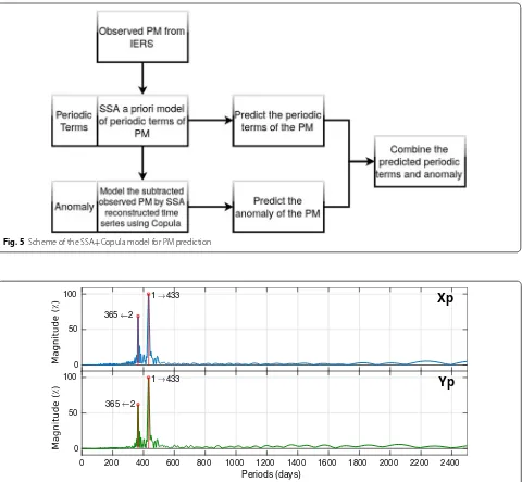
In this study, we defined an algorithm for PM prediction which is shown in Fig. 5. The observed PM time series can be split up into two parts. The first part is dealing with peri-odic effects such as Chandler wobble, annual variation, and influences of solid Earth tides and ocean tides on PM. The SSA is used to model the periodic terms of the PM. Then, the difference between the observed PM and SSA estimated data is modeled by using the Copula-based analysis method. After that, the periodic terms of PM are extrapolated using the SSA a priori model. Also, the anomaly part is predicted using the Copula-based model. Finally, the anomaly solution is added to the SSA-forecasted time series.

Therefore, the analysis of the data is divided into two main steps:

(1) SSA Periodic Terms Estimation

• Selecting window parameter (L) considering the

• Singular value decomposition of X,

• Selecting a proper group of singular values and

corresponding singular vectors,

• Reconstruction of X,

• Calculation of the trend by applying diagonal

averaging to X.

(2) Copula Anomaly Modeling

• Subtract the observed PM time series by

SSA-reconstructed time series,

• Forming the trajectory matrix of residual time

series using window length L and time delay of 1 day,

• Compute the marginal distribution of each

col-umn of the matrix,

• Transform data to the rank space,

• Compute the empirical Copula between the

col-umn i and i+1,

• Fit the theoretical Copula model by applying

appropriate goodness-of-fit tests,

• Compute the conditional Copula,

• Sample random data from the conditional

Cop-ula CDF and transfer the sample back to the data space using the inverse marginal,

• For each value of one input time series, one

obtains an ensemble of possible values for other time series.

Therefore, the final PM predicted data is the sum of the results of predicted periodic terms using SSA and pre-dicted anomaly using the Copula-based model.

SSA periodic terms estimation

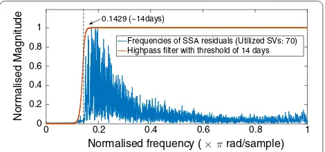
Window length selection is a crucial step in SSA which has a significant impact on the decomposition of the time series. The appropriate choice for L in a periodic time series with a period T is a window length proportional to the period, meaning that the L / T is an integer. Figure 6

depicts the main periods of PM time series (Golyandina and Zhigljavsky 2013). So, the Chandler period as the main period of both time series would be a reasonable

choice. Making the closest choice to the half of the length of the time series (if possible, least common multiple of the Chandler and annual periods) is recommended by Golyandina and Zhigljavsky (2013), but is avoided due to the processing time.

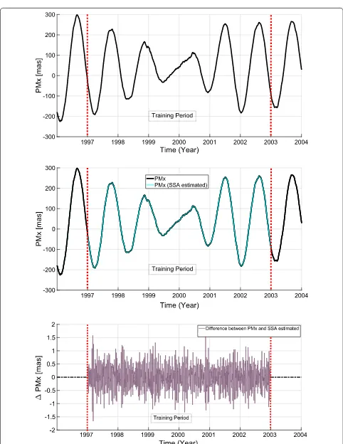
After selection of the window length, the number of singular vectors or empirical functions for reconstruction of the time series should be determined. The goal of this procedure is to find and apply a proper set of construc-tive components. Most significant periodicities as well as excitation mechanisms are rather low-frequency com-ponents and reveal their impact in the first few singular vectors while high-frequency components fall in later

Fig. 5 Scheme of the SSA+Copula model for PM prediction

200 400 600 800 1000 1200 1400 1600 1800 2000 2200 2400

0 50

100 1 433

_Xp

365 2

0 200 400 600 800 1000 1200 1400 1600 1800 2000 2200 2400

Periods (days)

0 50

100 1 433

_Yp

365 2

singular vectors. The singular value spectrum reflects the importance of each singular vector. Figure 7 suggests that in order to achieve an accuracy of about 1 mas in polar motion modeling, we need to utilize at least first 70 sin-gular vectors which correspond to using all components with periods more than or equal to 14 days.

Having the window length and the number of singular values determined, we construct the trajectory matrix. As it can be seen in Fig. 8 the data between the year of 1997 and 2003 is used as the training period. The cyan curve is the SSA-reconstructed PMx time series. Predic-tion of the future entries starts by adding initial guess of future entries to the end of the time series. Then, itera-tion of the SSA process is done until the result of two successive iterations has a difference less than a certain threshold. This will map the initial values to the estimated periodic terms of the time series. The residual part of the difference between original PMx time series and SSA esti-mated time series is named anomaly of PMx which has a stochastic behavior. Therefore, the anomaly part will be investigated by Copula-based technique.

Copula anomaly modeling

The anomaly part which is shown in Fig. 8 (lower panel) with dark violet is formed into a matrix with the same window length L. Then, the dependency structure between the rmcolumni and rmcolumni+1 is investigated

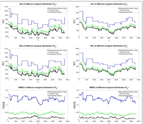
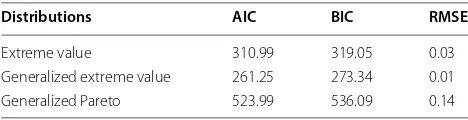
for the whole dataset. Modeling the joint dependence structure with Copulas requires fitting marginal distri-bution to data. In this study, three univariate distribu-tion funcdistribu-tions are considered: extreme value, generalized extreme value, and generalized Pareto distribution (see Table 2). To identify which univariate distribution is the best suitable for both PMx and PMy , the root-mean-square error is estimated and the goodness of fit is examined with the Akaike and the Bayesian information criteria (AIC and BIC).

and

(28) AIC=2k−ln(B)

where k denotes the number of the free parameters in the model. n is the sample size, and B is the maximized value of the likelihood function of the estimated model. The smallest amount of AIC or BIC, respectively, suggests the best fitting model or distribution. After estimation of the parameters by maximum likelihood approach, the AIC, BIC, and RMSE values are calculated for both PMx and PMy distribution. As it can be seen in Fig. 9, the general-ized extreme value (black) provides the best fit in com-parison with the generalized Pareto distribution function (blue) and extreme value distribution function (green). Furthermore, according to Tables  3 and 4, the result of the AIC, BIC, and RMSE confirmed that the generalized extreme value provides the best fit in both PMx and PMy distribution. Therefore, generalized extreme value distri-bution was selected in this study.

Estimating empirical Copula

Once the univariate marginal distribution is fitted, the dependence structure between the time series has to be investigated. The first step is to calculate the empirical Copula using Eq. (14). As it can be seen in Fig. 10, there is a scatter plot of two adjacent columns, and it shows a scatter linear dependency structure with the heavy tail. This kind of dependency structure can be correctly mod-eled using the Archimedean Copula.

Fitting a theoretical Copula function

The next step is fitting a theoretical bivariate Archime-dean Copula function with its parameters estimated by maximum likelihood approach. In this study, three dif-ferent theoretical Copula functions are tested (Fig. 11): Clayton, Frank, and Gumbel Copula. For the three dif-ferent Copula functions, the goodness-of-fit test, which is based on the Cramer–von Mises statistics, is applied. To evaluate the performance of the Copulas, 1000 values of the test statistics are sampled, and the proportion of values larger than Sn is estimated by calculating the cor-responding p values. The results based on Sn show that the performance of Frank Copula is slightly better than Gumbel and Clayton Copula with less error (Table 5).

365‑day‑ahead prediction

We utilized 6 years of observed PM time series, from Jan-uary 1997 to December 2002, for the 365-day-ahead pre-diction. To verify the reliability of this method, the results were compared with the IERS Bulletin A predictions (https ://datac enter .iers.org/web/guest /bulle tins/-/somos /5Rgv/versi on/6). The IERS Bulletin A contains the PM parameters and the predicted PM for one year into the future, and they are released every seven days by IERS (29)

BIC=k ln(n)−2 ln(B)

0 0.2 0.4 0.6 0.8 1

Normalised frequency ( rad/sample) 0

Frequencies of SSA residuals (Utilized SVs: 70) Highpass filter with threshold of 14 days 0.1429 (~14days)

Rapid Service/Prediction Center (RS/PC), hosted by the U.S. Naval Observatory (USNO) (Petit and Luzum 2010; Gambis and Luzum 2011). The predictions of PM from

the IERS Bulletin A were produced by LS + AR method. In the current prediction method, the PM prediction was the sum of the LS extrapolation model (including

Fig. 9 Marginal distribution’s goodness-of-fit test for PMx (left) and PMy (right). Generalized extreme value distribution is the black curve, green shows the extreme value distribution, and the blue curve is generalized Pareto distribution

Table 2 Marginal distributions

Distribution Formula Parameters

Extreme value (Kotz and Nadarajah 2000) f(x;µ,σ )=σ−1_exp(x−µ σ )exp

−expx−µ_σ Location µ scale σ

Generalized extreme value (Hosking et al. 1985)

f(x;µ,σ,ξ )= 1+ξ(

x−µ σ )

−1/ξ ifξ�=0 e−(x−µ)/σ ifξ=0

Location µ scale σ shape ξ

Generalized Pareto (Hosking and Wallis 1987)

f(x;σ,ξ )=f(ξ,µ,σ )(x)= σ1

1+ξ(x−_σµ)

−1 ξ−1

the Chandler period, annual, semiannual, terannual, and quarter annual terms), and the AR predictions of the LS extrapolation residuals (Kosek et al. 2007).

Discussion of results

In this study, we demonstrated the PM prediction by combination of SSA and Copula-based analysis method. Our method is tested based on the hindcast experiments using data from the past. Hence, we have calculated the results of our methods yearly for seven years of the test

Fig. 10 Scatter plot (left) two adjacent columns in the residual matrix. The empirical Copula (right) is estimated based on the dependency structure of two columns

Fig. 11 Theoretical Copula is fitted to the empirical Copula. The Copula parameter is 3.82, 15, and 3.61 for the Clayton, Frank, and Gumbel Copula, respectively

Table 3 Goodness-of-fit test for  marginal distribution of PMx

Distributions AIC BIC RMSE

Extreme value 574.60 582.66 0.04 Generalized extreme value 511.14 523.23 0.01 Generalized Pareto 758.22 770.31 0.13

Table 4 Goodness-of-fit test for  marginal distribution of PMy

Distributions AIC BIC RMSE

Extreme value 310.99 319.05 0.03 Generalized extreme value 261.25 273.34 0.01 Generalized Pareto 523.99 536.09 0.14

Table 5 Goodness-of-fit test for Copula model

Copula name Clayton Frank Gumbel

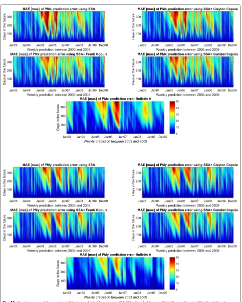
period 2003–2009 in comparison with Bulletin A PM prediction. As the prediction solutions of Bulletin A are available weekly, we would have approximately 52 time series of prediction for each year. So, Fig. 12 shows the mean value of MAE for each year. In Fig. 12, the Bulle-tin A solution is shown in black and the SSA predicted data in red. Also, the results of SSA+Copula are dis-played by green, blue, and pink for Clayton, Frank, and Gumbel Copula, respectively. Compared to the results from the IERS Bulletin A, the MAE of the predictions produced by the proposed method was smaller in dif-ferent short-, mid-, and long-term intervals for difdif-ferent cases (e.g., between 1 and 5 mas progression of PMx pre-diction for different time intervals in 2003). The better prediction performance of the SSA + Copula prediction may have been due to the modeling of the linear change of the Chandler and the annual oscillation amplitudes. Besides, the combination of SSA+Copula improves the SSA solution because of its ability to model the stochas-tic behavior of the anomaly part of the PM time series. However, the proposed method did not always perform better, especially in cases of long-term prediction where the quality of the results was not as good as we expected (see Fig. 12). This may have been caused by changes of the amplitudes of the periodic terms in this six-year time span where the SSA was not able to capture all features in order to predict more precisely we would have to increase the interval of training time. Figure 13 presents the abso-lute error of 365-day-ahead prediction between 2003 and 2009. Different patterns and features can be seen in our solution and Bulletin A solution. For instance, Bulletin A predicted PMx from January to March 2003 displays errors of more than 30  mas which cannot be found in our results, and there is a clear feature in PMx Bulletin A mean absolute error plot from August to December 2008 which does not appear in our prediction. How-ever, our predicted PM results indicate a periodic error in mid- and long-term predictions although the results of the combination SSA + Copula show smoother errors in comparison with the SSA results. To better understand this particular periodic error of our method, we plot Fig. 14 that demonstrates the improvement in the SSA + Copula predicted solution compared to Bulletin A. For each prediction epoch, if the difference between errors of Bulletin A prediction and errors of SSA/SSA+Copula is positive, it is considered as an improvement in predic-tion. Yellow color shows the progress in prediction in heat maps (see Fig. 14). The red color indicates where our method shows higher errors than Bulletin A in the pre-diction process. Also, the orange shows where both PM prediction techniques display the same amount of error. The results illustrate that SSA+Copula can improve the

accuracy of PM prediction in the different time intervals of prediction (short, mid, and long). Tables 6 and 7 indi-cate the success rate of PM prediction when using the SSA + Copula algorithm. The success rate of PM predic-tion is illustrated by the number of improvement in PM prediction (yellow) over the total number of PM predic-tion (yellow+ orange+ red).

The improvement in the prediction is approximately 40% on average. According to Malkin and Miller (2010), there is Candler Wobble phase variation in 1850, 1925, and 2005. So, probably it is the reason why the proposed prediction method losses accuracy around the year 2005. Also, as it can be seen in Tables 6 and 7 the success rate of PMx and PMy can be reached up to 64.99 and 46.66%, respectively.

Conclusions

The improvement in the Earth rotation prediction is a rel-evant, timely problem, as confirmed by the fact that the International Astronomical Union (IAU) Commission A2, the International Association of Geodesy (IAG), and the IERS have at present two Joint Working Groups on Prediction (JWG-P) and on Theory of Earth rotation and validation (JWG-ThER). According to the United Nations (UN) resolution in 2015, the primary objective of these JWGs is to assess and ensure the level of consistency of earth orientation parameter (EOP) predictions derived from theories with the corresponding EOP determined from analyses of the observational data provided by the various geodetic techniques. Therefore, accurate EOP predictions are essential to avoid any systematic drifts and/or biases between the international celestial and ter-restrial reference frames (ICRF and ITRF). The results illustrate that the proposed method could efficiently and precisely predict the PM parameters. As clearly demon-strated, the SSA + Copula algorithm shows better per-formance for PMx prediction in comparison with the SSA prediction. The Copula-based analysis is fully successful in its aim to increase the accuracy of PM prediction by modeling the stochastic part of the PM and subtract-ing PM by SSA-reconstructed time series. We suspect the main error contributions come from SSA extrapola-tion part. So, further investigaextrapola-tions about the SSA train-ing time will be required to clarify this issue. Also, SSA + Copula prediction method shows periodic errors, and these errors have a significant impact on the mean

(30)

Success rate of PM prediction

Fig. 14 Improvement of PMx and PMy prediction using SSA + Copula-based model compared with Bulletin A product for 2003, 2006, and 2009. The

improvement in prediction is shown by yellow color

Table 6 Success rate of PMx prediction [%]

Method\year 2003 2004 2005 2006 2007 2008 2009 Average

SSA 55.29 33.31 26.52 40.16 22.90 45.94 64.70 41.26 SSA + Clayton 61.71 33.88 31.91 40.17 22.91 45.96 64.95 43.07 SSA + Frank 58.31 34.31 33.61 42.50 22.91 45.97 64.99 43.22 SSA + Gumbel 55.90 33.81 28.31 41.00 22.90 45.94 64.97 41.83

Table 7 Success rate of PMy prediction [%]

Method\year 2003 2004 2005 2006 2007 2008 2009 Average

absolute error. Therefore, these occasional errors should be further investigated to have a noticeable progression in the PM prediction accuracy.

Abbreviations

ANN: artificial neural network; AR: autoregressive; CDF: cumulative distribution function; CLME: canonical maximum likelihood estimation; DORIS: Doppler Orbitography and Radiopositioning Integrated by Satellite; EOP: Earth orienta-tion parameters; EOP PCC: Earth orientaorienta-tion parameters predicorienta-tion compari-son campaign; GFZ: German Research Centre for Geosciences; GGOS: Global Geodetic Observing System; GNSS: Global Navigation Satellite Systems; IAG: International Association of Geodesy; ICRF: international celestial reference frame; IERS: International Earth Rotation and Reference Systems Service; IFME: Inference for Margins Estimation; LLR: Lunar Laser Ranging; LS: least squares; MAE: mean absolute error; RMS: root-mean-square; PM: polar motion; TRF: ter-restrial reference frame; VLBI: Very-long-baseline interferometry; SLR: Satellite Laser Ranging; SSA: singular spectrum analysis.

Authors’ contributions

SM did most of the data analysis and writing of the manuscript. MH carried out the SSA studies and wrote a part of the manuscript. SB conceived and designed the study. RH, JMF, and HS participated in the design of the study and helped to improve the manuscript. All authors read and approved the final manuscript.

Author details

1 _{GFZ German Research Centre for Geosciences, Potsdam, Germany.} 2 _Institute

for Geodesy and Geoinformation Science, Technische Universität Berlin, Berlin, Germany. 3 _{EPS, Applied Mathematics Department, University of Alicante,}

Campus de San Vicente, Alicante, Spain. 4 _{Department of Civil and}

Envi-ronmental Engineering, Norwegian University of Science and Technology, Trondheim, Norway.

Acknowledgements

We are grateful to the International Earth Rotation and Reference Systems Service (IERS) for providing the Polar motion data. We like to thank the two anonymous reviewers for their comments which helped to improve the paper.

Competing interests

The authors declare that they have no competing interests.

Funding

The corresponding author is supported by an offer of financial assistance by GFZ German Research Centre for Geosciences, Potsdam, Germany. SB and JF works were partially supported by Projects AYA2016-79775-P (AEI/FEDER, UE). Also, SB was supported by the European Research Council (ERC) under the ERC-2017-STG SENTIFLEX project (Grant Agreement 755617).

Publisher’s Note

Springer Nature remains neutral with regard to jurisdictional claims in pub-lished maps and institutional affiliations.

Received: 24 April 2018 Accepted: 27 June 2018

References

Akulenko L, Kumakshev S, Markov YG, Rykhlova L (2002) Forecasting the polar motions of the deformable earth. Astron Rep 46(10):858–865

Akyilmaz O, Kutterer H (2004) Prediction of earth rotation parameters by fuzzy inference systems. J Geodesy 78(1–2):82–93

Akyilmaz O, Kutterer H, Shum C, Ayan T (2011) Fuzzy-wavelet based prediction of earth rotation parameters. Appl Soft Comput 11(1):837–841

Angermann D, Seitz M, Drewes H (2010) Analysis of the DORIS contributions to IRTF2008. Adv Space Res 46(12):1633–1647

Bárdossy A, Li J (2008) Geostatistical interpolation using copulas. Water Resour Res 44(7):1–15

Bárdossy A, Pegram G (2009) Copula based multisite model for daily precipita-tion simulaprecipita-tion. Hydrol Earth Syst Sci 13(12):22–99

Barnes R, White A, Wilson C (1983) Atmospheric angular momentum fluctua-tions, length-of-day changes and polar motion. Proc R Soc Lond A 387(1792):31–73

Bizouard C, Gambis D, (2009) The combined solution c04 for earth orientation parameters consistent with international terrestrial reference frame 2005. In: Geodetic reference frames, Springer, pp. 265–270

Broomhead DS, King GP (1986) Extracting qualitative dynamics from experi-mental data. Phys D 20(2–3):217–236

Byram S, Hackman C (2012) High-precision GNSS orbit, clock and EOP estima-tion at the United States Naval Observatory. In: Posiestima-tion locaestima-tion and navigation symposium (PLANS), 2012 IEEE/ION, IEEE, pp. 659–663 Chen J, Wilson C (2005) Hydrological excitations of polar motion, 1993–2002.

Geophys J Int 160(3):833–839

Chin TM, Gross RS, Dickey JO (2004) Modeling and forecast of the polar motion excitation functions for short-term polar motion prediction. J Geodesy 78(6):343–353

Clayton DG (1978) A model for association in bivariate life tables and its appli-cation in epidemiological studies of familial tendency in chronic disease incidence. Biometrika 65(1):141–151

Coulot D, Pollet A, Collilieux X, Berio P (2010) Global optimization of core station networks for space geodesy: application to the referencing of the STR EOP with respect to ITRF. J Geod 84(1):31

Dickey J, Newhall X, Williams J (1985) Earth orientation from Lunar Laser Rang-ing and an error analysis of polar motion services. J Geophys Res Solid Earth 90(B11):9353–9362

Dow JM, Neilan RE, Rizos C (2009) The international GNSS service in a changing landscape of Global Navigation Satellite Systems. J Geod 83(3–4):191–198

Embrechts P, McNeil A, Straumann D (2002) Correlation and dependence in risk management: properties and pitfalls. In: Dempster MAH (ed) Risk management: value at risk and beyond, vol 1. Cambridge University Press, Cambridge, pp 176–223

Escarela G, Carriere JF (2003) Fitting competing risks with an assumed Copula. Stat Methods Med Res 12(4):333–349

Freedman A, Steppe J, Dickey J, Eubanks T, Sung L-Y (1994) The short-term prediction of universal time and length of day using atmospheric angular momentum. J Geophys Res Solid Earth 99(B4):6981–6996

Gambis D, Luzum B (2011) Earth rotation monitoring, UT1 determination and prediction. Metrologia 48(4):S165

Genest C, Favre A-C (2007) Everything you always wanted to know about Copula modeling but were afraid to ask. J Hydrol Eng 12(4):347–368 Genest C, Rivest L-P (1993) Statistical inference procedures for bivariate

Archi-medean Copulas. J Am Stat Assoc 88(423):1034–1043

Giacomini E, Härdle W, Spokoiny V (2009) Inhomogeneous dependence mod-eling with time-varying Copula. J Bus Econ Stat 27(2):224–234 Golyandina N, Zhigljavsky A (2013) Singular Spectrum Analysis for time series.

Springer-Verlag, Berlin

Golyandina N, Nekrutkin V, Zhigljavsky AA (2001) Analysis of time series struc-ture: SSA and related techniques. Chapman and Hall, New York Gross RS (2015) Earth rotation variations—long period. Phys Geod 11:215–261 Gross RS, Fukumori I, Menemenlis D (2003) Atmospheric and oceanic

excita-tion of the earth’s wobbles during 1980–2000. J Geophys Res Solid Earth 108(B8):2370

Hosking JR, Wallis JR (1987) Parameter and quantile estimation for the general-ized Pareto distribution. Technometrics 29(3):339–349

Hosking JR, Wallis JR, Wood EF (1985) Estimation of the generalized extreme-value distribution by the method of probability-weighted moments. Technometrics 27(3):251–261

Jaworski P, Durante F, Härdle WK, Rychlik T (2010) Copula theory and its applications. In: proceedings of the workshop held in Warsaw, 25–26 September 2009, Vol. 198, Springer Science & Business Media

Joe H (1997) Multivariate models and multivariate dependence concepts. CRC Press, Boca Raton

Joe H, Xu JJ (1996) The estimation method of inference functions for margins for multivariate models, Technical report, Department of Statistics, Uni-versity of British Columbia

Kalarus M, Schuh H, Kosek W, Akyilmaz O, Bizouard C, Gambis D, Gross R, Jovanović B, Kumakshev S, Kutterer H et al (2010) Achievements of the earth orientation parameters prediction comparison campaign. J Geod 84(10):587–596

Kosek W, McCarthy D, Luzum B (1998) Possible improvement of earth ori-entation forecast using autocovariance prediction procedures. J Geod 72(4):189–199

Kosek WI, Kalarus M, Niedzielski T, Capitaine N (2007) Forecasting of the Earth orientation parameters: comparison of different algorithms. Observatoire de Paris, Paris

Kotz S, Nadarajah S (2000) Extreme value distributions: theory and applica-tions. World Scientific, Singapore

Laux P, Vogl S, Qiu W, Knoche H, Kunstmann H (2011) Copula-based statistical refinement of precipitation in RCM simulations over complex terrain. Hydrol Earth Syst Sci 15(7):2401–2419

Lee T-H, Long X (2009) Copula-based multivariate GARCH model with uncor-related dependent errors. J Econom 150(2):207–218

Malkin Z, Miller N (2010) Chandler wobble: two more large phase jumps revealed. Earth Planets Space 62(12):943–947

Mathews P, Buffett BA, Herring TA, Shapiro II (1991) Forced nutations of the earth: influence of inner core dynamics: 1. Theory. J Geophys Res Solid Earth 96(B5):8219–8242

Modiri S, Lorenz C, Sneeuw N, Kunstmann H, (2015) Copula-based estima-tion of large-scale water storage changes: exploiting the dependence structure between hydrological and grace data. In: EGU general assembly conference abstracts, Vol. 17

Nelsen RB (2007) An introduction to copulas. Springer Science & Business Media, Berlin

Nilsson T, Böhm J, Schuh H (2010) Sub-diurnal earth rotation variations observed by VLBI. Artif Satell 45(2):49–55

Nilsson T, Böhm J, Schuh H (2011) Universal time from VLBI single-baseline observations during CONT08. J Geod 85(7):415–423

Nilsson T, Heinkelmann R, Karbon M, Raposo-Pulido V, Soja B, Schuh H (2014) Earth orientation parameters estimated from VLBI during the CONT11 campaign. J Geod 88(5):491–502

Patton AJ (2006) Modelling asymmetric exchange rate dependence. Int Econ Rev 47(2):527–556

Patton AJ (2009) Copula-based models for financial time series. In: Mikosch T, Kreiß J-P, Davis RA, Andersen TG (eds) Handbook of financial time series. Springer, Berlin, pp 767–785

Petit G, Luzum B (2010) IERS conventions (2010), Technical report, Bureau International des poids et mesures sevres (France)

Plag H-P, Pearlman M (2009) Global geodetic observing system: meeting the requirements of a global society on a changing planet in 2020. Springer, Berlin

Rachev S, Mittnik S (2000) Stable Paretian models in finance. Willey, New York Rodriguez JC (2007) Measuring financial contagion: a copula approach. J

Empir Finance 14(3):401–423

Schuh H, Behrend D (2012) VLBI: a fascinating technique for geodesy and astrometry. J Geodyn 61:68–80

Schuh H, Böhm S (2011) Earth rotation. In: Gupta HK (ed) Encyclopedia of solid earth geophysics. Springer, Dordrecht, pp 123–129

Schuh H, Schmitz-Hübsch H (2000) Short period variations in earth rotation as seen by VLBI. Surv Geophys 21(5–6):499–520

Schuh H, Ulrich M, Egger D, Müller J, Schwegmann W (2002) Prediction of earth orientation parameters by artificial neural networks. J Geod 76(5):247–258

Seitz F, Schuh H (2010) Earth rotation. In: Xu G (ed) Sciences of geodesy-I. Springer, Berlin, pp 185–227

Sklar M (1959) Fonctions de repartition an dimensions et leurs marges. Publ. Inst. Statist. Univ. Paris 8:229–231

Stamatakos N (2017) IERS rapid service prediction center products and ser-vices: improvement, changes, and challenges, 2012 to 2017. In: Proceed-ings of the Journées Systèmes de référence spatio-temporels’ Trivedi PK, Zimmer DM et al (2007) Copula modeling: an introduction for

practitioners. FoundTrends® Economet 1(1):1–111

Vautard R, Yiou P, Ghil M (1992) Singular-Spectrum Analysis: a toolkit for short, noisy chaotic signals. Phys D 58(1–4):95–126

Verhoest NE, van den Berg MJ, Martens B, Lievens H, Wood EF, Pan M, Kerr YH, Al Bitar A, Tomer SK, Drusch M et al (2015) Copula-based downscaling of coarse-scale soil moisture observations with implicit bias correction. IEEE Trans Geosci Remote Sens 53(6):3507–3521

Vogl S, Laux P, Qiu W, Mao G, Kunstmann H (2012) Copula-based assimilation of radar and gauge information to derive bias-corrected precipitation fields. Hydrol Earth Syst Sci 16(7):2311–2328

Wahr JM (1982) The effects of the atmosphere and oceans on the earth’s wobble—I. Theory. Geophys J Int 70(2):349–372

Wahr JM (1983) The effects of the atmosphere and oceans on the earth’s wobble and on the seasonal variations in the length of day—II. results. Geophys J Int 74(2):451–487

Wang W, Wells MT (2000) Model selection and semiparametric inference for bivariate failure-time data. J Am Stat Assoc 95(449):62–72

Willmott CJ, Matsuura K (2005) Advantages of the mean absolute error (MAE) over the root mean square error (RMSE) in assessing average model performance. Clim Res 30(1):79–82

Włodzimierz H (1990) Polar motion prediction by the least-squares collocation method. In: Boucher C, Wilkins GA (eds) Earth rotation and coordinate reference frames. Springer, US, pp 50–57

Xu X, Zhou Y, Liao X (2012) Short-term earth orientation parameters predic-tions by combination of the least-squares, AR model and Kalman filter. J Geodyn 62:83–86

Yue S (1999) Applying bivariate normal distribution to flood frequency analy-sis. Water Int 24(3):248–254

Zhang L, Singh VP (2007) Bivariate rainfall frequency distributions using Archi-medean Copulas. J Hydrol 332(1–2):93–109