Geomagnetic depth sounding in the Northern Apennines (Italy)
E. Armadillo1, E. Bozzo1, V. Cerv3, A. De Santis2, D. Di Mauro2, M. Gambetta1, A. Meloni2, J. Pek3, and F. Speranza2
1Dipartimento per lo studio del terrirorio e delle sue risorse, Viale Benedetto XV, 5-16132 Genova, Italy 2Istituto Nazionale di Geofisica e Vulcanologia, Via di Vigna Murata, 605-00143 Rome, Italy
3GFU CSAV, 141 31 Praha 4, Czech Republic
(Received January 11, 2000; Revised January 11, 2001; Accepted February 6, 2001)
A Geomagnetic Depth Sounding (GDS) survey covering the Northern Apennines of Italy has been carried out in the period 1992–94. Induction arrows maps and hypothetical event Fourier maps were constructed to obtain an electromagnetic imaging of this area. Since the two dimensional (2-D) character comes out from those maps for periods greater than 32 minutes, a 2-D inverse modeling was carried out. The model responses show that a deep conductive layer (>5000 S) underlies the Apennine chain at about 20 km depth. The transition between the Adriatic and the Tyrrhenian domains is marked by a rather sharp vertical offset in this conducting layer. In the northwest sector of the studied area an anomalous high conductivity behavior is superimposed on the regional trend, which corresponds to the geothermal field of Larderello-Travale.
1.
Introduction
In the northern Apennines, the surface of the upper crust down to a few km is well known by drill hole data (Anelliet al., 1994). Good quality information is also available for the mantle structure, down to about 500 km depth. Here seis-mic tomography revealed the unravel pattern of descend-ing slabs and asthenosphere upwelldescend-ings (e.g. Mele et al., 1997; Lucenteet al., 1999). On the other hand, few con-straints are available for the intermediate depth structure, at the lower crust/upper mantle interval. Seismic reflec-tion/refraction data obtained so far are susceptible of con-trasting interpretations and their quality progressively re-duces along depth, approaching the Moho (e.g. Pialliet al., 1998). In order to obtain independent results to constrain the crustal/lithospheric structure underneath central Italy, the Geomagnetic Depth Sounding (GDS) technique was applied since it is a valid tool to access geoelectrical information at depths of investigations not reachable with other geophysi-cal methods.
GDS provides useful information on the distribution of the electrical conductivity in the lower crust and upper man-tle by means of magnetovariational (MV) observations at the Earth’s surface. The electrically conducting Earth modifies magnetic variations originating from natural sources in the magnetosphere and the ionosphere via electromagnetic in-duction. As known, in a uniform halfspace the skin depth δ = 30.2(T/σ)1/2is the characteristic penetration depth in km of a signal with periodT (in hours) in a subsoil with con-ductivityσ(in S/m). Models of vertical and lateral conduc-tivity profiles can lead to mapping fluid electrolytes, highly conductive minerals and anomalous temperature gradients, and may aid in improving the understanding of regional
geo-Copy right c The Society of Geomagnetism and Earth, Planetary and Space Sciences (SGEPSS); The Seismological Society of Japan; The Volcanological Society of Japan; The Geodetic Society of Japan; The Japanese Society for Planetary Sciences.
dynamic and tectonic features (Gough, 1989, 1992; Hjelth and Korja, 1993).
A visual comparison of the morphology of MV field from different sites yields preliminary information of the spatial distribution of electrical conductivity over the investigated area (Gough, 1989). In this paper we present the first pro-posal for 2-D electrical resistivity structure over the North-ern Apennines by means of GDS method based on an array of 14 three-component geomagnetic stations. The paper is organised as follows. After this introduction we start with a description of the geologic and tectonic setting of the inves-tigated area. We then describe how measurements and data analysis have been carried out, showing results in the form of induction arrows maps and Fourier maps in the hypothet-ical event technique, followed by a 2-D inversion modelling. We finally conclude with some considerations and specula-tions.
2.
Tectonics of the Northern Apennines
In the frame of the central Mediterranean geodynamic evolution, the tectonic setting of the Northern Apennines is thought to result from the complex interplay of the Africa-Europe collision, roll-back of isolated slab fragments, as-thenospheric upwelling and collapse of thickened belts (e.g. Jolivetet al., 1998).
From late Cretaceous, the convergence between Eurasian and African margins caused the closure of Western Tethys and the consumption of the Adriatic promontory margins. From late Miocene, shortening was confined in the external zones of the Apennine chain. Conversely the more internal (western) sectors were characterized by an extensional tec-tonics and a significant magmatic activity (e.g. Serriet al., 1993).
The structural setting of the central Mediterranean region has been investigated by means of various geophysical
10°
Moho Isobaths (km) Overthrusting Front of the Moho
subducting plate overriding plate
50 m
Fig. 1. Main structural and geographical features of Italy.
methods. Deep seismic soundings have been extensively carried out, in particular, reflection and refraction profiles were obtained in the seventies (Lavecchia, 1988 and refer-ences therein). These preliminary interpretations were lately confirmed and improved by studies based on surface wave scattering (Sneider, 1988) and tomography (Babuska and Plomerov`a, 1990; Amato et al., 1993; Spakman et al., 1993). Gravimetric, magnetic, heat flow, petrologic and geo-chemical models (e.g. Cassinis et al., 1991; Serri et al., 1993; Molinaet al., 1994; Mongelliet al., 1998) aided in re-fining the geophysical features of the Central Mediterranean zone.
In the Apennines, middle Miocene to Pleistocene east-ward frontal accretion was simultaneous to back-arc exten-sion and related foundering of the Tyrrhenian Sea. In the Northern Apennines, extensional tectonics progressively fragmented the internal compressive fronts, and produced several syn-rift basins in Tuscany and in the axial belt filled by “neoautochthonous” Neogene sediments. A normal thickness (35–40 km) crust characterizes the Adriatic fore-land and the external Northern Apennines, whereas the Northern Tyrrhenian Sea and Tuscany are formed by thinned (20–25 km) continental crust (Pialliet al., 1998). The
down-ward prosecution of the Adriatic lithosphere below the Northern Apennines is traceable by seismic tomography as a steep slab reaching at least 500 km depth (Lucenteet al., 1999). West of the steep slab, asthenospheric material is inferred to raise beneath the Northern Tyrrhenian Sea up to 30 km depth and to laterally migrate eastward beneath the central-eastern belt itself (Mele et al., 1997). This asthenospheric upwelling accounts both for the Miocene-Pleistocene magmatism in the Northern Tyrrhenian Sea and Tuscany (Serriet al., 1993) and the high thermal flow (100– 200 on average and locally up to 1000 mW/m2) observed nowadays in the same area (Mongelliet al., 1989) (see Fig. 1 for the main structural and geographical features of Italy).
3.
Measurements
An array of 14 MV stations, from the Tyrrhenian to the Adriatic coast, covering an area of about 40000 km2 was
A
A'
B
B'
30 km
N
Adriatic Sea
Tyrrhenian Sea
Fig. 2. Investigated area in Central Italy with locations of magnetometer stations (with station codes) and profiles used in the 2-D model.
variations were sampled at 5 Hz with a 10 s anti-aliasing fil-ter of seven 0.1 normalized Bessel functions and stored at the rate of 1 value per minute. Since the time of the sur-vey almost coincided with a minimum of solar activity, the magnetometers operated for at least 4 months at each site to obtain a satisfactory number of geomagnetic events to ana-lyze.
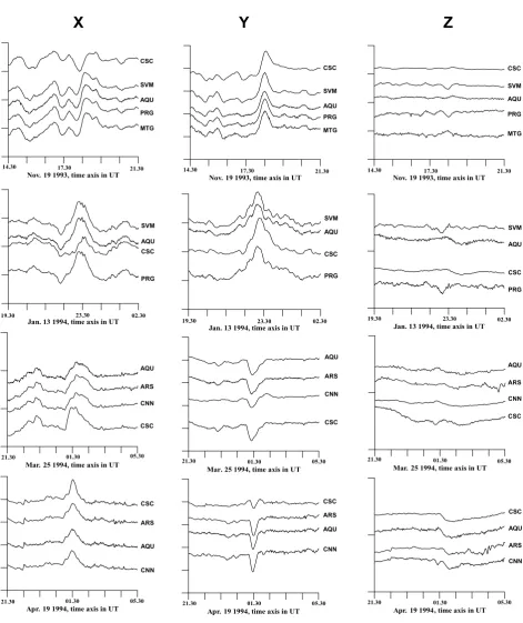
Figure 3 shows some selected samples of stacked mag-netograms from various magnetic disturbance events. Such events are grouped according to the simultaneously working stations at the indicated site. The horizontal magnetic com-ponents are almost uniform over the array, but some phase shifts are visible and can be indicative of 3-D conductivity distribution at shallow depths (Fig. 3). The vertical compo-nent amplitudes at SVM, AQU, and PRG show larger signals as compared to other sites (e.g. CSC, ARS, CNN). These suggest a large lateral conductivity contrast within the study area. The station CSC shows large phase shift as well as amplitude variation with respect to the neighboring stations in all three components.
4.
Data Analysis
4.1 Induction arrows
From each site, various 512-minute records of X,Y, Z Earth’s magnetic components, characterizing magnetically disturbed intervals, were extracted. After Fast-Fourier trans-forming all components into the frequency domain, the sin-gle station transfer functions A(f)and B(f)between the vertical and horizontal Cartesian Fourier components were estimated for each frequency f:
Z(f)= A(f)X(f)+B(f)Y(f)+δZ(f). (1)
In order to minimize the residualδZ(f), a standard least squares method (Everett and Hyndman, 1967) and a robust estimation approach (Egbert and Booker, 1986) were
de-rived.
Figure 4 shows the transfer functions at the short-medium term period (T = 16 and 32 minutes) and medium-long period (T =64 and 85.3 minutes) in the form of real and imaginary reversed induction arrows (or Parkinson arrows; e.g. Parkinson, 1989), so as to point towards zones of high conductivity (Lilley and Arora, 1982). A multivariate anal-ysis (Egbert and Booker, 1989) on 46 simultaneous events recorded at the four northernmost sites has suggested that estimates of the induction arrows are not biased by the pos-sible presence of anomalous field in horizontal components of the inducing field (Armadilloet al., 1995).
The local pattern of the real induction arrows (Fig. 4) is consistent with a “coast effect” (Parkinson and Jones, 1979). These arrows point away from the central axis of the Italian peninsula, towards the Adriatic and the Tyrrhenian Sea re-spectively, while at the central stations the magnitudes are generally low. Nevertheless, peculiar features in this overall pattern indicate that the inductive response of the regional 2-D structure of the area is superimposed on the coast effect and well detectable.
Induction vector magnitudes near the NE coast are larger than those near the SW coast. This behavior is rather un-expected for a coast effect, at least on two counts: first the coast effect is in general of the same intensity at opposite coast lines, second, the observed difference is also in con-trast with the depth of the two adjacent seas (the depth of the Adriatic Sea in the NE of Italy ranges 50–100 m while the depth of the Northern Tyrrhenian Sea in the SW ranges 500–1000 m). Moreover, the induction vectors in the eastern sector decrease in magnitude and then invert their direction on a relatively short distance.
From the point of period dependence of induction arrows the four stations close to the Adriatic Sea (PNB, PRG, SVM, TRM) show a similar behavior: the magnitude of the induc-tion arrows increases with the decrease of the period while in their directions they constantly point perpendicularly to the coast line. On the contrary, the induction arrows on the Tyrrhenian side show a scattered trend. In fact, their magni-tude values do not increase regularly with the frequency (or decrease with period) and, moreover, the arrow’s azimuths at nearby stations point toward different directions. There are many rapid changes in the direction of the induction arrows for both real and imaginary parts across very short distances, especially at short to intermediate periods (stations PNB and PRG, PTG, and CNN). This is evidence for a 3-D character of the shallower geoelectrical configuration.
Among the central stations, CSC and AQU show consis-tent behavior. At higher frequency, they both turn from S to E-SE and magnitude increases only at the shortest periods. The RTI arrow has a direction similar to ARS while MTG points toward E at the shorter periods. CDC turns from W to N at the higher frequency (Fig. 4).
For what concerns longer periods (last two boxes in Fig. 4) the behavior of induction arrows evidences a 2-D structure, taking standard errors into account.
4.2 Hypothetical event technique
Nov. 19 1993, time axis in UT
14.30 17.30 21.30
AQU
PRG
MTG SVM CSC
Nov. 19 1993, time axis in UT
14.30 17.30 21.30
AQU PRG
MTG SVM CSC
Nov. 19 1993, time axis in UT
14.30 17.30 21.30
AQU
PRG
MTG SVM CSC
Jan. 13 1994, time axis in UT
19.30 23.30 02.30
AQU SVM
PRG CSC
Jan. 13 1994, time axis in UT
19.30 23.30 02.30
AQU SVM
PRG CSC
Jan. 13 1994, time axis in UT
19.30 23.30 02.30
AQU SVM
PRG CSC
Mar. 25 1994, time axis in UT
21.30 01.30 05.30
AQU
ARS
CNN
CSC
Mar. 25 1994, time axis in UT
21.30 01.30 05.30
AQU
ARS
CNN
CSC
Mar. 25 1994, time axis in UT
21.30 01.30 05.30
AQU
ARS
CNN
CSC
Apr. 19 1994, time axis in UT
21.30 01.30 05.30
AQU
CNN ARS CSC
Apr. 19 1994, time axis in UT
21.30 01.30 05.30
AQU
CNN ARS CSC
Apr. 19 1994, time axis in UT
21.30 01.30 05.30
AQU
CNN ARS CSC
X
Y
Z
Fig. 3. Four samples of time variations of the north (X), east (Y), and vertical (Z) magnetic field components recorded simultaneously at various sites (in the ordinates, each interval unit between two scale marks is 50 nT).
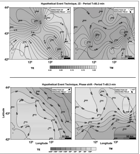
(1) with a unitary horizontal magnetic field constrained to be linearly polarized over the array. We attempt two directions of polarization nearly parallel and orthogonal to the strike of the most evident tectonic formation, i.e. the Apennine chain (57◦and 147◦clockwise from north), respectively. The re-sulting contour maps, for both amplitude and phase shift values for periods of 85.3 and 16 minutes, are presented in Figs. 5 and 6. They allow a preliminary pattern recognition in spatial conductivity distribution. Since EM induction in
an elongated conductor is maximized by a source magnetic field directed at right angles to the strike of structure, the maps may be used to confirm the existence of a body (or any geological structure) with elongated dimensions in the direction orthogonal to the imposed field. The induced per-pendicular field (Figs. 5 and 6, left hand side) enhances the coast effect to 57◦. The effect is visible both in the amplitude and in the phase shift map.
distin-Fig. 4. Real and imaginary induction arrows (with error ellipses) for periods of 16, 32, 64, 85.3 minutes.
guish between local induction and channeling. Perturbation (channeling) of the regional current flow in a thin sheet of laterally variable conductance produces an anomalous verti-cal field in phase (or with a phase shift of 180◦) with the re-gional current and hence uniform over the array, while only its amplitude will vary (Banks and Beamish, 1984). On the contrary, strong differences in the phase values may indicate the dominance of local induction effects (e.g. Aroraet al., 1998).
The induced field perpendicular to 57◦N (Figs. 5 and 6; left hand side) enhances both the regional 2-D structure of the area and the effect of the sea, since both have the same strike. An attempt to distinguish between the two sources has been performed by the 2-D inversion as discussed in the next section, where the coast effect has been modeled. The phase values, especially at the coastal stations, are quite uniform, approaching−180◦ in the Adriatic sector and 0◦
val-42º 43º 44º
12º 13º
RDC
PTG
CNN
RTI
ARS RDD
MTG
CSC
AQU PNB
CDC
PRG
SVM
TRM
12º 13º
RDC
PTG
CNN
RTI
ARS RDD
MTG
CSC
AQU PNB
CDC
PRG
SVM
TRM
12º Longitude 13º
RDC
PTG
CNN
RTI
ARS RDD
MTG
CSC
AQU PNB
CDC
PRG
SVM
TRM
42º 43º 44º
L
a
tit
ude
12º Longitude 13º
RDC
PTG
CNN
RTI
ARS RDD
MTG
CSC
AQU PNB
CDC
PRG
SVM
TRM
0.00 0.05 0.10 0.15 0.20
Hypothetical Event Technique, |Z| - Period T=85.3 min
Hypothetical Event Technique, Phase shift - Period T=85.3 min 50 km
DIRECTION OF
INDUCING FIELD 57º
50 km DIRECTION OF
INDUCING FIELD 57º
50 km DIRECTION OF INDUCING FIELD
147º
50 km DIRECTION OF INDUCING FIELD
147º
TE TM
-220º -180º -140º -100º -60º -20º 20º 60º 100º
TE TM
Fig. 5. Fourier maps of magnitude values (top) and phase (down) of the vertical componentZfor the periodT=85.3 minutes in the hypothetical event technique polarized at 57◦(left) and 147◦(right).
ues are smaller than the other coastal ones. This causes a clearly visible interruption of the SE-NW trend of amplitude isolines.
When the 147◦N horizontal polarization is chosen (Fig. 5, right hand side), for the 85.3 minutes period the phase shift values at ARS, RTI, CSC, AQU, TRM, SVM sites are neg-ative while they are positive at the other stations. This con-figuration highlights a belt of high gradient between the two site groups. At the shorter period, (Fig. 6, right) phase shift values increase towards south and north while they are strongly negative at MTG and CSC.
5.
2-D Inversion
In order to estimate the regional electrical conductivity distribution beneath the investigated area, a 2-D modelling technique was applied to two profiles (A–A’ and B–B’ in Fig. 2) perpendicular to the Apenninic trend. The experi-mental data show the following features:
42º 43º 44º
12º 13º
RDC
PTG
CNN
RTI
ARS RDD
MTG
CSC
AQU PNB
CDC
PRG
SVM
TRM
12º 13º
RDC
PTG
CNN
RTI
ARS RDD
MTG
CSC
AQU PNB
CDC
PRG
SVM
TRM
42º 43º 44º
Lat
it
u
de
12º Longitude 13º
RDC
PTG
CNN
RTI
ARS RDD
MTG
CSC
AQU PNB
CDC
PRG
SVM
TRM
0.00 0.05 0.10 0.15 0.20 0.25 0.30 0.35
Hypothetical Event Technique, Phase shift - Period T=16 min Hypothetical Event Technique, |Z| - Period T=16 min
50 km
DIRECTION OF
INDUCING FIELD 57º
50 km
DIRECTION OF
INDUCING FIELD 57º
50 km
DIRECTION OF INDUCING FIELD
147º
12º Longitude 13º
RDC
PTG
CNN
RTI
ARS RDD
MTG
CSC
AQU PNB
CDC
PRG
SVM
TRM
50 km
DIRECTION OF INDUCING FIELD
147º
-220º -180º -140º -100º -60º -20º 20º 60º 100º
TE TM
TE TM
Fig. 6. Fourier maps of magnitude values (top) and phase (down) of the vertical componentZfor the periodT=16 minutes in the hypothetical event technique polarized at 57◦(left) and 147◦(right).
2. Induction arrows indicate partly three-dimensional dis-tribution. In several stations the component of the in-duction arrows parallel to the profiles is quite compa-rable with the perpendicular one.
3. For all four studied periods the imaginary part of the induction vectors is comparable with the real compo-nent.
For the inversion process, only the component of the in-duction arrows parallel to the profiles was considered and
only the projections of the arrows of the closest sites to each profile were used for computation. Moreover, we inverted the same four periods (16, 32, 64, 83.5 minutes) considered for the transfer function analysis.
Fig. 7. 2-D resistivity models for the two profiles across Central Italy. Resistivity scaled inm (see the gray scale). Locations of the sites (indicated by their acronyms) and their distances in km from the West coast (origin) are plotted on the upper horizontal axis. The vertical lower case axis indicates depth in km. Small black boxes, numbered from 1 to 5 are referred to the same imposed conditions, listed in Section 4, as initial features for the modelling. Blocks forming the lower crust conductor are marked with number 6; blocks number 7 in the Eastern sector are not part of this layer (see the discussion in the text). Block numbered 8 indicates a conductive structure under the Adriatic sea.
geomagnetic induction problem (Cerv and Pek, 1981; Pek, 1987). No smoothing was applied since the relatively small number of involved parameters implicitly regularized the problem.
The procedure requires an initial electrical and geometri-cal model from which it evolves to a final one. The common features imposed on all 2-D starting models can be summa-rized as follows (Fig. 7):
1) two marine expanses of low resistivity (0.25m) with mean depth of 1 km (Tyrrhenian Sea) and 0.2 km (Adri-atic Sea);
2) a high resistivity layer (1000–3000 m) beneath the Italian peninsula with maximum depth of 5 km rep-resented by Meso-Cenozoic carbonates (e.g. Consiglio Nazionale delle Ricerche, 1991);
3) a conductive (sedimentary) layer (1–3m) beneath the Adriatic foreland, some kilometers thick due to clayey-terrigenous sediments (e.g. Ballyet al., 1986);
4) a layer of rather resistive crustal material (1000–2000 m) beneath the belt which, reaching the maximum depth of 35–40 km, follows approximately the Moho profile thinning toward the west (e.g. Lavecchia, 1988);
5) a deeper conductive layer (∼10m) which likely rep-resents the asthenophere (e.g. Meleet al., 1997).
Only the first feature has been maintained constant during the inversion, while all the others (2–5) have been consid-ered as electrical and geometrical free parameters.
Figure 7 shows the resulting models of the inversion for the two profiles. In Fig. 8 the experimental data (points with error bars) and the final 2-D model responses (solid line) are compared along the profile B–B’ for the four periods. The main effect of the inferred conductive bodies in the models can be summarized in the following way:
1. Below the conductive Adriatic sediments the data still require a more conductive body. The response of the model without this conductive body is shown in Fig. 8, by the dash dot line. In this case, at the eastern coastal stations it is not possible to reach a good fit with to the experimental real and imaginary parts of the induction vectors. Without the conductive sediments the real part is too small while the imaginary part is in an opposite direction with respect to the observed one. The latter consideration is important since the imaginary part of the induction vectors controls the depth of the conduc-tive body.
-1 Im [Z/H], T=64 minutes, rms=0.10
Re [Z/H], T=32 minutes, rms=0.10
Re [Z/H], T=64 minutes, rms=0.05
Re [Z/H], T=85.3 minutes, rms=0.25
Im [Z/H], T=16 minutes, rms=0.17
Im [Z/H], T=32 minutes, rms=0.11
Im [Z/H], T=85.3 minutes, rms=0.05 Re [Z/H], T=16 minutes, rms=0.11
Fig. 8. Comparison betweenZ/Hratio obtained from the final 2-D model (solid line) and the experimental values (points with error bars) for the profile BB’ in the four periods. The other curves represent the responses of the model: without the conductive body below the Adriatic sea (dash-dot line), without the conductive body below the inland sector and without the body west from Apennines (small and large dashed line, respectively).
the experimental data but worse than the final model. The conductive body below the Apennines (S >5000 Siemens) allowed us to model the quick changes of the induction vectors in the eastern part of the model on a relatively short distance (jointly with the conductor below Adriatic sea). Clearly, due to the large station spacing along the two sections AA’ and BB’, a struc-tural interpretation of the very shallow conductive dis-tribution cannot be attempted.
In order to evaluate the significance of the model features, we also adopted an efficient variant (Siripunvaraporn and Egbert, 2000) of the Occam inversion approach (De Groot-Hedlin and Constable, 1990). The method looks for models fitting the data and having the minimum structure, that is models which are as smoothest as possible. Practically this approach gives the lower bounds on the amount of structure required by data and so the resolving power of GDS method in the actual contest can be estimated.
Results for the two sections AA’ and BB’ are shown in Fig. 9 and should be compared with the models of Fig. 7. From the analysis of the two different inversion methods, it follows that the onshore high conductivity contiguous blocks in Fig. 7 can be considered as a continuous layer and that this layer is necessary to justify actual data.
Moreover, the main features shown in Fig. 7 are qualita-tively confirmed in the minimum structure models of Fig. 9.
The enhanced conductive layer deepens from the west to the east sector and also the local shallow anomaly close to RDC and RDD stations is required by data.
On the contrary, the new results of REBOCC inversion (Fig. 9) confirm that the conductivity of the Adriatic sedi-ments alone can explain the observed data and that the con-ductive body (marked with number 8 in Fig. 7) under the conductive Adriatic sediments is not necessary.
6.
Discussion
The MV response in the Northern Apennines area reveals a 2-D regional electrical conductivity pattern superimposed on more local and shallow 3-D anomalies. The structural in-terpretation of these features is partly hindered by the coast effect, since the coast and the main structures have a simi-lar strike. However, in the 2-D resistivity sections of Figs. 7 and 9, the conductivity of the sea is introduced and mod-eled to evaluate and distinguish its contribution to the 2-D regional conductivity pattern.
The models highlight the presence of some enhanced con-ductivity blocks in the crust (1–10m at a depth of about 20 km, labeled with number 6 in both the sections of Fig. 7), which are necessary to explain the experimental data, as shown in Section 4. Taking into account the limited number of stations along both sections and the results of the min-imum structure REBOCC inversion (Fig. 9), the series of contiguous blocks can be considered as a continuous layer in the lower crust.
The origin and significance of an enhanced conductive layer in the lower continental crust is still an open ques-tion: different causes have been proposed in the recent lit-erature. At a global scale the most plausible explanations are related to saline pore fluids, graphitic horizons or phyl-losilicate minerals (e.g. Jones, 1992; Hyndmanet al., 1993; ELEKTB Group, 1997; Losito and Muschietti, 1998). The general conductance of the lower crust is in the range 10– 1000 S. In particular, in Precambrian areas, these values are found between 100–300m while in Phanerozoic ar-eas they commonly are in the range 10–30m (Marquis and Hyndman, 1992). In the studied area we have obtained the values lower than the lowest Phanerozoic values. This result may suggest an underestimation of the thickness of the layer of the 2-D model. It is known from theoretical studies (e.g. Edwardset al., 1981) that the depth to the base of a conductive layer is resolved with the greatest uncer-tainty. Since also the minimum structure models (Fig. 9) confirm the anomalous high conductivity values, some par-ticular mechanism should be considered to account for our data. In fact, very often the conduction mechanism is strictly dependent on the local structure and can be also related to partial melting in volcanic and geothermal areas or to the presence of metallic oxides and hydrated minerals (e.g. Losito and Muschietti, 1998).
In the case of a pore fluids conduction mechanism (Hyndman and Shearer, 1989) as a source of enhanced con-ductivity in the lower crust, this should be expected at the transition from hydrostatic to lithostatic pore pressures, that occurs at the brittle-ductile boundary. The latter, on the basis of general temperature versus depth models, should corre-spond to the 350–400◦C isotherm (Marquis and Hyndman,
1992).
Our results show that the conductive layer deepens from the Tyrrhenian domain to the Adriatic one. The model depths of the top of the layer (Fig. 7) are consistent with the estimated values of the brittle-ductile boundary as inferred basically from seismic and heat flow data. The very low thickness of the crustal brittle layer in the peri-Tyrrhenian region is proven by shear seismic wave attenuation measure-ments (Mele et al., 1997) and by the extremely high heat flow (over 100 mW m−2) observed in Tuscany and in gen-eral in the Western Apennines (Pasqualeet al., 1993). From heat flow data, ductile behavior is estimated to begin at∼10 km where temperatures of around 370–390◦C are reached. On the contrary, in the external zone of the Northern Apen-ninic arc, the brittle-ductile transition is expected at 25–32 km and at temperatures around 320–380◦C (Pasqualeet al., 1997).
Moreover, the transition between the Adriatic and the Tyrrhenian domains appears to be characterized by a rather sharp offset of the conductive layer (visible in both the sec-tions A–A’, B–B’ of Fig. 7) approximately under the Apen-nine watershed. Seismic experiments have shown that the top of the lower crust follows the same trend of the crust-mantle boundary (Barchiet al., 1998). So, even if the Moho discontinuity cannot be resolved by our data, the offset of the conductive layer correlates well with the Moho offset of about 10–15 km (Lavecchia, 1988), which marks the transi-tion between the two domains.
In the west sector, the thermal origin of the anomaly can be invoked to account for the modeled higher electrical ductivity values compared to the average mid-crustal con-ductors ones. From the analysis of the seismic CROP 03 experiment results, Barchi et al.(1998) note in this sector an acoustically well defined top of the lower crust that ap-pears to be related to partially molten material indicating that the source of the heat is at shallow depth and that the crust-mantle processes of interaction affect the entire lower crust.
Nevertheless, this explanation does not work for the east-ern sector, where heat flow data are not anomalous, even if according to Federico and Pauselli (1998) the thermal in-fluence of the subducted Adriatic slab below the Tyrrhenian one is not negligible: this could explain in part the high con-ductivity values inferred from the GDS modeling also in this sector.
litho-spheric structure independently inferred by seismological studies. By coupling the information from subcrustal seis-micity (Selvaggi and Amato, 1992), shear wave attenua-tion (Meleet al., 1997), and P wave tomographic images (Lucente et al., 1999), it results that asthenosphere rises obliquely, eastward “intruding” the northern Apennine litho-sphere. The mechanism of asthenospheric upwelling is coin-cident to those expected by crust/mantle delamination mech-anisms (e.g. Channell and Mareschal, 1989). On the other hand, the horizontal extension (about 10×20 km2) of the seismic surface is less than that of the conductive layer which is modeled to extend up to RDD station, although the resolution of conductive layer is not so good. In the same area, a peak in the residual heat flow density is well known and defines the Larderello-Travale geothermal anomaly (e.g. Mongelli et al., 1989) with values up to 1000 mW m−2. The heat flow anomaly has been modeled by Mongelliet al.(1998) with an intrusive body of hot asthenospheric ma-terial 15–20 km in diameter extending from 5 to 40 km in depth.
Another relevant feature in the models is the presence of a conductivity block (about 10m) in the Adriatic sector at depths with top at 7 km and with a lateral extension of about 20–30 km. The block is visible in both the sections in Fig. 7 (marked with label 7), beneath PNB station (section A–A’), and TRM, SVM stations (section B–B’). It cannot be identi-fied with the lower crust, since it is too shallow with respect to the estimated brittle-ductile transition in this region (25– 32 km according to Pasqualeet al., 1997). At such depths a fluid/melt layer is inappropriate since this part of the crust is made by “basement” rocks at temperature lower then 300– 400◦C (Cataldiet al., 1995). The conductivity enhancement in this area and at this depth may correspond to the transition between the Meso-Cenozoic carbonates and the underlying Si-rich metamorphic rocks for which the minimum melting temperature should be around 700◦C.
7.
Concluding Remarks and Future Work
Concerning the reliability of the interpretations, it must be considered that the responses of a few GDS sites were projected with the unpredictable influence of the near sur-face inhomogeneities. In such pattern, few points impli-cate the assumption of limited approximations over a com-pound configuration especially beneath the surrounding seas since the observations were limited on the land part. More-over, fictitious results can be conducted when 2-D analy-ses are performed over data in 3-D structures (see Ting and Hohman, 1981; Wannamakeret al., 1984 for examples on TE-mode magnetotelluric data to which GDS induction ar-rows correspond).
More detailed evaluations of the topography and conduc-tivity of the sea in addiction to the information from the as-sessment of a map of global conductance in this area (from MT data, if available, and from borehole logs) and, finally, a denser coverage of measurement sites will be the starting points for a better investigation of the area, together with the performing of a more suitable 3-D modelling approach. Having focused our interest to the essential features required in both two inversions beneath the land part, this paper has to be considered as a first step to establish some key points,
within an electromagnetic approach, in this complex frame.
Acknowledgments. We would like to express a special thank to Dr. Jurgen Watermann from the Danish Meteorological Institute for his helpful suggestions, to Mr. Giorgio Caneva and Mr. Enzo Zunino from the Dipartimento Scienze Terra, University of Genoa, and Mr. Luigi Magno from INGV for their collaboration in the field work. We would like to acknowledge the appropriate comments of the EPS Editor Dr. Y. Ogawa, of Prof. B. R. Arora, and an anony-mous reviewer and that allowed the substantial improvement of the paper. Finally, we are also grateful to all farmers, ground owners and town councils that hosted the automatic equipments across the region under study.
References
Amato, A., B. Alessandrini, and G. B. Cimini, Teleseismic wave tomog-raphy of Italy, inSeismic Tomography. Theory and Practice, edited by H. M. Iyer and K. Hirahara, pp. 361–396, Chapman & Hall, Cambridge, 1993.
Anelli, L., M. Gorza, M. Pieri, and M. Riva, Subsurface well data in the northern Apennines (Italy),Mem. Soc. Geol. It.,48, 461–471, 1994. Armadillo, E., E. Bozzo, and M. Gambetta, Tecniche di analisi statistiche
applicate ai dati magnetovariazionali per lo studio di strutture di con-ducibilit`a litosferiche, Proceeding 13th GNGTS Meeting, Rome, 143– 150, 1995.
Arora, B. R., A. Rigoti, I. Vitorello, A. L. Padilha, N. B. Trivedi, and F. H. Chamalaun, Magnetometer study array in North-Northeast Brazil: con-ductivity image building and functional Induction modes,Pageoph,152, 349–375, 1998.
Babuska, V. and J. Plomerov`a, Tomographic studies of the upper mantle beneath Italian region,Terra Nova,2, 569–576, 1990.
Bailey, R. C., G. D. Edwards, G. D. Garland, R. Kurtz, and D. Pitcher, Electrical conductivity studies over a tectonically active area in Eastern Canada,J. Geomag. Geoelectr.,26, 125–146, 1974.
Bally, A. W., L. Burbi, C. Cooper, and R. Ghelardoni, Balanced sections and seismic reflection profiles across the central Apennines,Mem. Soc. Geol. It.,35, 257–310, 1986.
Banks, R. J. and D. Beamish, Local and regional induction in the British Isles,Geophys. J. R. astr. Soc.,79, 539–553, 1984.
Barchi, M., G. Minelli, and G. Pialli, The CROP 03 profile: a synthesis of results on deep structures of the northern Apennines,Mem. Soc. Geol. It.,52, 383–400, 1998.
Batini, F., G. Bertini, G. Giannelli, E. Pandelli, and M. Puxeddu, Deep structure of the Larderello field: contribution from recent geophysical and geological data,Mem. Soc. Geol. It.,5, 219–235, 1983.
Cameli, G. M., I. Dini, and D. Liotta, Brittle/ductile boundary from seismic reflection lines of southern Tuscany (Northern Apennines, Italy),Mem. Soc. Geol. It.,52, 153–162, 1998.
Cassinis, R., G. Pialli, M. Broggi, and M. Prosperi, Dati gravimetrici a grande scala lungo la fascia del profilo: interrogativi sull’assetto della crosta e del mantello, inStudi preliminari all’acquisizione dati del pro-filo CROP 03 Punta Ala - Gabicce, edited by G. Pialli, M. Barchi, and M. Menichetti, St. Geol. Cam., University of Camerino, Camerino, vol. I1, 41–48, 1991 (in Italian).
Cataldi, R., F. Mongelli, P. Squarci, L. Taffi, G. Zito, and C. Calore, Geothermal ranking of Italian territory,Geothermics,24(1), 115–129, 1995.
Cerv, V. and J. Pek, Numerical solution of the two-dimensional inverse geomagnetic problem,Studia Geophys. Geod.,25, 69–80, 1981. Channell, J. E. T. and J. C. Mareschal, Delamination and asymmetric
litho-spheric thickening in the development of the Tyrrhenian Rift, in Alpine Tectonics,Geol. Soc. Spec. Publ.,45, 285–302, 1989.
Consiglio Nazionale delle Ricerche, Structural model of Italy, scale 1:500,000, Progetto Finalizzato Geodinamica, Roma, 1991.
De Groot-Hedlin, C. and C. G. Constable, Occam’s inversion to gener-ate smooth, two dimensional models from magnetotelluric data, Geo-physics,55, 1613–1624, 1990.
Edwards, R. N., R. C. Bailey, and G. D. Garland, Conductivity anomalies: lower crust or asthenophere?,Phys. Earth Planet. Inter.,25, 263–272, 1981.
Egbert, G. D. and J. R. Booker, Multivariate analysis of geomagnetic array data. 1 The response space,J. Geophys. Res.,94(B10), 14227–14247, 1989.
functions,Geophys. J. R. astr. Soc.,87, 173–194, 1986.
ELEKTB Group, KTB and the electrical conductivity of the crust,J. Geo-phys. Res.,102, 18289–18305, 1997.
Everett, J. E. and R. D. Hyndman, Geomagnetic variation and electrical conductivity structure in Southwestern Australia,Phys. Earth Planet. In-ter.,1, 23–34, 1967.
Federico, C. and C. Pauselli, Thermal evolution of the Northern Apennines (Italy),Mem. Soc. Geol. It.,52, 267–274, 1998.
Gough, D. I., Magnetometer array studies, Earth structures and tectonic process,Rev. Geophys.,27, 141–157, 1989.
Gough, D. I., Electromagnetic exploration for fluids in the Earth’s crust,
Earth Sci. Rev.,32, 3–18, 1992.
Hjelth, S. E. and T. Korja, Lithospheric and upper-mantle structures, results of electromagnetic sounding in Europe,Phys. Earth Planet. Inter.,79, 137–177, 1993.
Hyndman, R. D. and P. M. Shearer, Water in the lower continental crust: modelling magnetotelluric and seismic reflection results,Geophys. J. In-ter.,98, 343–365, 1989.
Hyndman, R. D., L. L. Vanyan, G. Marquis, and L. K. Law, The origin of electrically conductive lower continental crust: saline water or graphite?,
Phys. Earth Planet. Inter.,81, 325–344, 1993.
Jolivet, L., C. Faccenna, B. Goff´e, M. Mattei, F. Rossetti, C. Brunet, F. Storti, R. Funiciello, J. P. Cadet, N. d’Agostino, and T. Parra, Mid-crustal shear zones in postorogenic extension: Example from the north-ern Tyrrhenian Sea,J. Geophys. Res.,103, 12123–12160, 1998. Jones, A. G., Electrical conductivity of the continental lower crust, in
Con-tinental Lower Crust, edited by D. M. Fountain, R. I. Arculus, and R. W. Kay, pp. 81–143, Elsevier, Amsterdam, 1992.
Lavecchia, G., The Tyrrhenian-Apennines system: structural setting and seismotectogenesis,Tectonophys.,147, 263–296, 1988.
Lilley, F. E. and B. R. Arora, The sign convention for quadrature Parkinson arrows in Geomagnetic induction Studies,Rev. Geophys. Space Phys.,
20, 513–518, 1982.
Losito, G. and M. Muschietti, Is the illite group the cause of high electrical conductivity in certain lithospheric areas?,Ann. Geofis.,41(3), 369–381, 1998.
Lucente, F. P., C. Chiarabba, G. B. Cimini, and D. Giardini, Tomographic constraints on the geodynamic evolution of the Italian region,J. Geo-phys. Res.,104, 20307–20327, 1999.
Marquis, G. and R. D. Hyndman, Geophysical support for aqueous fluids in the deep crust: seismic and electrical relationships,Geophys. J. Int.,
110, 91–105, 1992.
Mele, G., A. Rovelli, D. Seber, and M. Barazangi, Shear wave attenua-tion in the lithosphere beneath Italy and surrounding regions: Tectonic implications,J. Geophys. Res.,102, 11863–11875, 1997.
Molina, F., E. Armando, R. Balia, O. Batteli, E. Bozzo, G. Budetta, G. Caneva, M. Ciminale, N. De Florentiis, A. De Santis, G. Dominici, M. Donnaloia, A. Elena, V. Iliceto, R. Lanza, M. Loddo, A. Meloni, E.
Pinna, G. Santarato, and R. Zambrano, Geomagnetic survey of Italy at 1979.0 repeat station network and magnetic maps, Internal report ING publication 554, Rome, pp. 43, 1994.
Mongelli, F., G. Zito, N. Ciaranfi, and P. Pieri, Interpretation of heat flow density of the Apennine chain, Italy,Tectonophys.,164, 267–280, 1989. Mongelli, F., F. Palumbo, M. Puxeddu, I. M. Villa, and G. Zito, Interpreta-tion of the geothermal anomaly of Larderello, Italy,Mem. Soc. Geol. It.,
52, 305–318, 1998.
Parkinson, W. D., The analysis of single site induction data,Phys. Earth Planet. Inter.,53, 360–364, 1989.
Parkinson, W. D. and F. W. Jones, The geomagnetic coast effect,Rev. Geo-phys. Space Phys.,17, 1999–2015, 1979.
Pasquale, V., M. Verdoja, P. Chozzi, and P. Augliera, Dependence of the seismotectonic regime on the thermal state in the Northern Italian Apen-nines,Tectonophys.,217, 31–41, 1993.
Pasquale, V., M. Verdoja, P. Chozzi, and G. Ranalli, Rheology and seis-motectonic regime in the northern central Mediterranean,Tectonophys.,
270, 239–257, 1997.
Pek, J., Numerical inversion of 2D MT data by models with variable geom-etry,Phys. Earth Planet. Inter.,45, 193–203, 1987.
Pialli, G., M. Barchi, and G. Minelli, Results of the CROP03 deep seismic reflection profile,Mem. Soc. Geol. It.,52, 657 pp., 1998.
Selvaggi, G. and A. Amato, Subcrustal earthquakes in the Apennines (Italy): Evidence for a still active subduction?,Geophys. Res. Lett.,19, 2127–2130, 1992.
Serri, G., F. Innocenti, and P. F. Manetti, Geochemical and petrological ev-idence of the subduction of delaminated adriatic continental lithosphere in the genesis of the Neogene Quaternary magmatism of central Italy,
Tectonophys.,223, 117–147, 1993.
Siripunvaraporn, W. and G. Egbert, REBOCC: An efficient data-subspace inversion for two-dimensional magnetotelluric data,Geophysics,65(3), 791–803, 2000.
Sneider, R., Large scale waveform inversions of surface-waves for lateral heterogeneity—II: Application to surface waves in Europe and the Mediterranean,J. Geophys. Res.,93(B10), 12067–12080, 1988. Spakman, W., S. van der Lee, and R. van der Hilst, Travel-time tomography
of the European-Mediterranean mantle down to 1400 km,Phys. Earth Planet. Inter.,79, 3–74, 1993.
Ting, S. C. and G. W. Hohmann, Integral equation modeling of three-dimentional magnetotelluric response,Geophysics,46, 182–197, 1981. Wannamaker, P. E., G. W. Hohmann, and S. H. Ward, Magnetotelluric
re-sponse of three-dimensional bodies in layered earth,Geophysics, 48, 1517–1533, 1984.