Earth Planets Space,53, 75–89, 2001
Three-component OBS-data processing for lithology and fluid prediction
in the mid-Norway margin, NE Atlantic
Eivind Berg1∗, Lasse Amundsen1, Andrew Morton1∗, Rolf Mjelde2, Hideki Shimamura3, Hajime Shiobara3∗∗, Toshihiko Kanazawa4∗∗, Shuichi Kodaira3∗∗∗, and Jan Petter Fjellanger2∗∗∗∗
1Statoil, Trondheim, Norway
2Inst. of Solid Earth physics, University of Bergen, Norway 3Inst. for Seismology and Volcanology, Hokkaido University, Sapporo, Japan
4Lab. Earthquake Chemistry, Tokyo University, Japan
(Received January 24, 2000; Revised September 25, 2000; Accepted October 18, 2000)
In 1992, a comprehensive three-component ocean bottom seismic survey was performed in the central and northern area of the Vøring Basin, offshore mid-Norway, NE Atlantic. An important part of the data acquisition program consisted of a local survey with 20 Ocean Bottom Seismographs (OBS) dropped at approximately 200 m interval in 1300 m water depth. The main purpose of the local survey was to acquire densely sampled P- and S-wave reflection data above a seismic flatspot anomaly observed earlier, in order to more accurately predict if hydrocarbons could be related to it. The conventional reflection data processing methods applied to the vertical components included predictive deconvolution in order to attenuate low frequency ringing, near offset mute and a series of constant velocity stacks in order to obtain the optimal velocity function. The final result is a “trouser” shaped, high resolutionVzstacked section with minor influence of water multiples. The inline (Vx) component contains no
strong multiples, and extensive near trace muting was hence not necessary to apply for this component. Velocity analysis together with ray-tracing modelling indicate that P-S-converted shear waves (reflections) represent the dominant mode. The results of the interpretation and modelling indicated aVp/Vs-ratio of approximately 2.6 in
the overburden, which suggests domination of partly unconsolidated shale, while theVp/Vs-ratio in the assumed
reservoir was approximately 1.8, which indicates a more sand dominated facies. Outside the flatspot area a higher
Vp/Vs-ratio ratio (approximately 2.0) was estimated, indicating that hydrocarbons could be present in the assumed
reservoir.
1.
Introduction
Recording the seismic wavefield at the sea-floor using mul-ticomponent receivers has several advantages compared to conventional near surface recording (Caldwell, 1999); im-provedP-wave imaging due to lower background noise level, better azimuth distribution and more possibilities for removal of receiver ghost and multiples, use ofP-S-converted waves to image below shallow gas and to map geological boundaries with low acoustic impedance forP-waves.
Furthermore, it is well known that obtaining estimates of
S-wave velocities for sedimentary rocks in addition to P -wave velocities to a certain extent enables prediction of lithol-ogy and fluids (e.g. Nur and Simmons, 1969; Christensen and Fountain, 1975; Spencer and Nur, 1976; Kern, 1982; Christensen, 1984; Crampin, 1990). In several different sed-imentary sequences it has been shown that theVp/Vs-ratio
can be related to the sand/shale ratio; aVp/Vs-ratio of 1.6
rep-∗Now at SB Geophysical a.s., Trondheim, Norway. ∗∗Now at Earthquake Research Inst., Tokyo University, Japan. ∗∗∗Now at JAMSTEC, Yokosuka, Japan.
∗∗∗∗Now at Norsk Hydro, Bergen, Norway.
Copy right cThe Society of Geomagnetism and Earth, Planetary and Space Sciences (SGEPSS); The Seismological Society of Japan; The Volcanological Society of Japan; The Geodetic Society of Japan; The Japanese Society for Planetary Sciences.
resenting sand and aVp/Vs-ratio of 2.0 representing shale.
Presence of hydrocarbons tend to decrease theVp/Vs-ratio
(Neidell, 1985).
TheVp/Vs-ratio can be estimated indirectly from marine
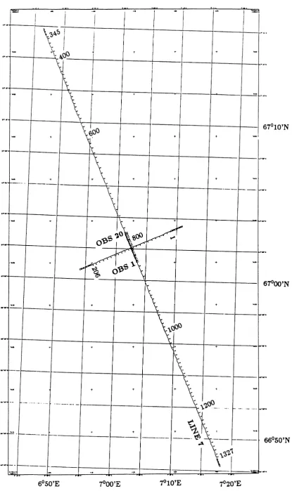
seismic data by analysing Amplitude-Versus-Offset (AVO), but in order to perform more precise direct measurements, three-component (3-C) recorders on the ocean bottom are needed. In 1992 a comprehensive 3-C OBS (Ocean Bot-tom Seismograph) survey was performed in the central and northern area of the Vøring Basin, mid-Norway margin, NE Atlantic, the largest sedimentary basin off Norway remaining to be explored (Fig. 1). The data acquisition program con-sisted of three parts, with one regional and one semi-regional part providing the large basin coverage (Digraneset al., 1996; Mjeldeet al., 1996, 1997a, b). The third part consisted of a local survey with 20 OBSs dropped along surface seismic line VB-08-89 at approximately 200 m interval in 1300 m water depth (Fig. 2). The main purpose of the local survey was to acquire densely sampled P- and S-wave reflections above a seismic flatspot anomaly observed earlier in surface seismic data, in order to more accurately predict if hydrocar-bons could be present. Flatspots are often taken as indicators of the presence of hydrocarbons, and they are interpreted as boundaries between different types of pore-fluid, e.g. gas and water (Caldwell, 1999). The survey was undertaken by
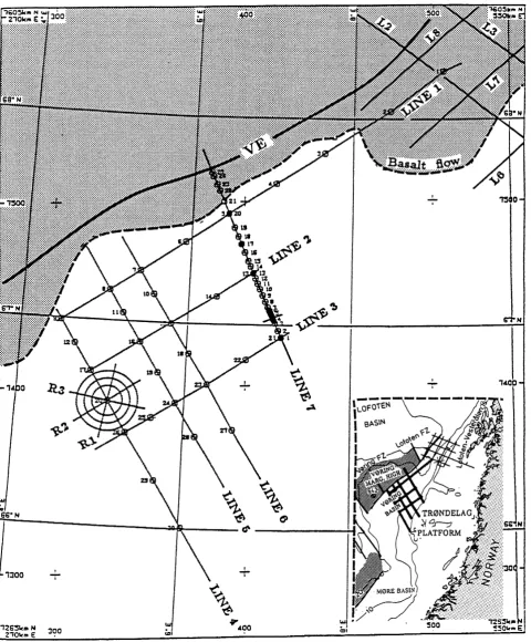
Fig. 1. Location of the OBS-profiles acquired during the survey in 1992. The local data presented in this paper were acquired along a part of Line 7. The framed area shows the geographical location of the 1992 profiles (bold lines), as well as regional OBS-profiles acquired off Lofoten in 1988 (thin lines). VE=Vøring Escarpment.
entists from the Universities of Bergen, Hokkaido and Tokyo as well as from Statoil’s Research Centre in Trondheim. The data were converted from its original analogue tape format to a standard digital format at Hokkaido University. Fur-ther processing (described in this paper) has been applied
using Advance Geophysical’s (now Landmark’s) ProMAX and VSP software in Statoil’s Research Centre to produce stacked seismic sections of the vertical and inline horizontal components of the data.
E. BERGet al.: OBS-PROCESSING FOR LITHOLOGY AND FLUID PREDICTION 77
Fig. 3. Part of reflection profile VB-08-89 (migrated stack processed by Merlin Geophysical). The OBSs in the local study were located above the indicatedflatspot. The reservoir is assumed to be bounded by the flatspot, the intra Campanian Unconformity (top reservoir) and the fault.
how conventional (surface) reflection data processing meth-ods applied to 3-C OBS-data can be used for lithology and
fluid predictions.
2.
Data Acquisition
The OBSs used in the survey were developed at Labo-ratory for Ocean Bottom Seismology, Hokkaido University, and Laboratory for Earthquake Chemistry, Tokyo University (Shimamura, 1988; Kanazawa, 1993). Each OBS contains gimbal-mounted, oil damped, three-component geophones, two variable speed tape drives, an amplifier with gain set-tings of 49 dB and 79 dB, and an internal clock calibrated to a master clock onboard the vessel. Other equipment, such as ballast, a release mechanism and homing aids, are incorpo-rated for the deployment and retrieval of the instruments.
For the data presented in this paper, the analogue seismic signals were recorded with a high tape drive speed, allow-ing frequencies up to 40 Hz to be preserved, and the OBSs to remain active on the sea-floor for almost 8 days. As the OBSs were deployed in deep water (ca. 1300 m depth), the ballast was increased to 40 kg to speed up their descent and prevent the instruments from drifting laterally too far from the release point on the surface. Their position on the sea bed was obtained by measuring the ship to transponder dis-tance from 19 different surface positions, using a measured acoustic velocity-depth function and then performing non-linear inversion to minimise the travel time errors between observed and ray-traced times (Shiobaraet al., 1997). The
E. BERGet al.: OBS-PROCESSING FOR LITHOLOGY AND FLUID PREDICTION 79
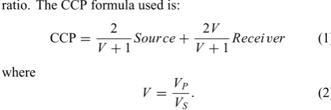
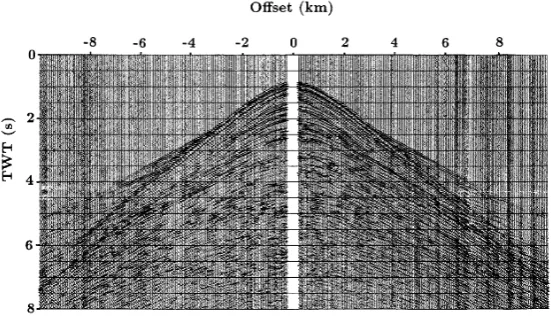
Fig. 5. Raw data recorded on the vertical component of OBS 10.
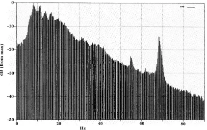
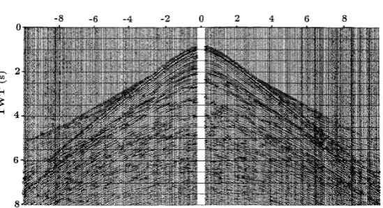
Fig. 6. Raw data recorded on one of the horizontal components of OBS 10. (The data on the other horizontal component is qualitatively very similar and is hence not presented).
true OBS positions were generally found to be at distances less than 100 m from their deployment positions with an er-ror in the positioning of about 10 m. 20 OBSs were deployed along the position of line VB-08-89 with an approximate sep-aration of 200 m (Fig. 2; Table 1), centered above theflatspot indicated in Fig. 3.
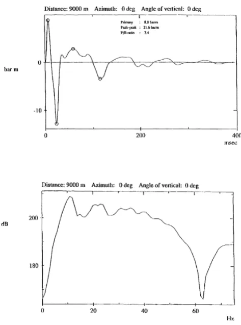
The data presented in this paper were recorded in the high gain setting using an air-gun array (7 air-guns) with a total volume of 32.1 l (1956i n3) towed at a depth of 12 m. The
source signature and amplitude spectrum are shown in Fig. 4. During the shooting of the ca. 56 km long line the vessel attempted to maintain a constant speed of 1.6 knots andfire the guns every 60 seconds, corresponding to ca. every 50 m.
However, this speed was not maintainable in strong currents, and the speed of the vessel had to be gradually increased to 2.8 knots.
3.
Multicomponent OBS Processing
3.1 Data input
re-Fig. 7. Fold of stack for CDP line.
covered, and the data for OBS 11 was discarded as it appeared very noisy due to problems with the gain settings. The raw data for the vertical and one of the horizontal components of OBS 10 are presented in Figs. 5 and 6.
Initially each tape was read into ProMAX, preserving the offset andfieldfile numbers in the trace headers. From each of the field files channels 1–3 were extracted: channel 2 being the vertical component and channels 1 and 3 the two perpendicular horizontal components. After studying some of the common OBS gathers, the input data were further limited to a maximum offset of 15 km and a time of 12 s. For each OBS a dataset was created with a surface shot point and coordinate relative to the conventional seismic line acquired in 1989 (VB-08/08A-89). This provided the basis for a line geometry, which was needed to obtain a stack from the data. Table 1 shows the shot point numbers and coordinates used. By creating a geometry and combining the 17 OBS datasets into one, it was possible to extract individual components and attempt to process the data with conventional techniques.
3.2 Geometry application
The next step in the processing sequence consisted of cre-ating the geometry necessary for processing and stacking the data. The detailed procedure for the geometry application is presented in Appendix A.
For this dataset the average fold for 50 m bin width is around 80, if all offsets are included in the stack (Fig. 7). Discarding traces not contributing to the stack at the target level leaves a fold of stack of around 25.
For asymmetric or Common Conversion Point (CCP) bin-ning of the horizontal components, the calculation of the CCP x coordinate includes constants derived from the Vp/Vs
-ratio. The CCP formula used is:
CCP= 2
When theVp/Vs-ratio equals one, this equation gives nor-mal CMP numbering. A geometry was created for the hori-zontal component data with aVp/Vs-ratio of 1.0, 1.75, 2.0, 2.5 and 2.75.
3.3 Processing of the vertical component
Thefirst attempts to identify theflatspot were in the re-ceiver domain of the vertical components. Some efforts were made to NMO correct these gathers both with a velocity function taken from the VB-08/08A-89 migrated stack, and a simplified velocity function based on four key horizons identified in the gathers. An attempt to stack the data (in the receiver domain) before the geometry was created, indicated that the flatspot could be identified if the multiple energy was removed. As the spatial sampling is irregular, multiple attenuation can only be accomplished by inner trace muting. Thisfirst simple stack (Fig. 8) showed the major horizons and a dipping event interpreted as the intra Campanian un-conformity (Mjeldeet al., 1997a) located above theflatspot, which cannot be seen clearly.
E. BERGet al.: OBS-PROCESSING FOR LITHOLOGY AND FLUID PREDICTION 81
Fig. 8. Initial“receiver gather”stack (after application of deconvolution; see Fig. 10). The stacked trace for each OBS has been displayed four times.
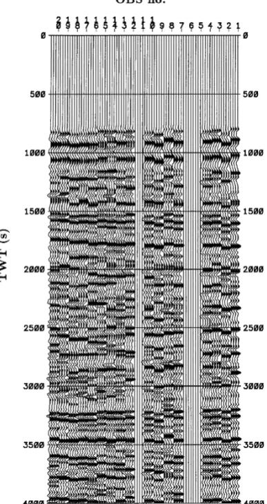
parameters found were a 250 ms operator with 50 ms gap for predictive deconvolution. After analysing the OBS am-plitude spectra (Fig. 9), a minimum phase Butterworth band passfilter of 5 to 35 Hz with slopes of 18 and 72 dB/octave was applied. Figure 10 shows the vertical component of OBS 10 after application of deconvolution and band passfiltering. Top and bottom mutes were individually picked on the OBS gathers to remove the high-energy direct arrivals and the sea bottom multiple (Fig. 11). The resulting“trouser”
shaped stack has strongly improved primary signal around the target interval at 2700 ms. Figure 12(a) shows a stack of the data with a single velocity function taken from VB-08/08A-89. With these parameters applied to a CMP-sorted dataset, it was possible to perform velocity analysis and a much more detailed velocityfield could be picked. The lo-cations for the analysis were, on average, every 10th CMP (500 m) and the analysis was performed on a super gather of 5 CMPs, summed with a 50 m offset bin. This improved the offset sampling to give a more regularly sampled gather and hence a better velocity analysis. The velocity function was picked on a normalized semblance display, with an in-teractive stack and gather for quality control. The gather
display was difficult to utilize due to the muting and sam-pling, and the velocity functions were generally difficult to pick consistently due to the low fold of the primary energy. The difference in semblance between signal and noise was slight, and the display (colour contouring) and scaling (time normalising) was thus important. Figure 13(a) shows a typi-cal semblance display taken from the data. Constant velocity stacks were run on the whole line to help distinguish events, and a simple velocityfield was derived from them. As the quality of the picking was difficult to evaluate during the anal-ysis, and the data are very sensitive to muting (especially the top mute) and velocity, it was found that the best test of a velocityfield and/or mute was to actually perform the stack. In the CMP domain it is also possible to derive and apply trim statics before stacking. These simple correlation statics are derived along a horizon-following window. CMP trim statics provide a powerful tool to optimise the stack, but the result is heavily dependant on the parameters chosen. Dif-ferent horizons were selected, but the event at 1500 ms with a 3000 ms window over 3 CMPs provided the most consis-tent results. The maximum static allowed was set to 40 ms, and during the analysis many traces reached this limit. It was found that a better stack was obtained if those traces that reached the maximum had their static shift set to zero. Fig-ure 12(b) shows a residual corrected stack. Once a reasonable set of statics was derived, velocity analysis was performed on a residual corrected dataset, and the velocityfield wasfinely tuned. Efforts to improve the post stack data were made, since these data represent regular zero offset traces at 50 m increments. F-X deconvolution (random noise removal) and post stack F-Kfiltering (dipping noise attenuation) were per-formed, but did not produce any significant improvement.
From the vertical component stack it can be seen that the event at roughly 1500 ms is approximatelyflat. Picking a horizon along this event allows a static shift to be applied us-ing the“Horizon Flattening”tool (Fig. 12(c)). This improves the overall appearance of the events, theflatspot appears more horizontal, and the stack ties better with the conventional sur-face seismics. The stack with residual statics and the F-K
filter wasfinally migrated with an Explicit Finite Difference Time Migration algorithm, as shown in Fig. 12(d).
3.4 Processing of the horizontal components
Considerable efforts were made in order to rotate the hor-izontal components into inline and crossline components. This work is described in detail in Appendix B. Since this study was not conclusive, both the unrotated and rotated datasets have been used in the further processing. The pro-cessing of the horizontal components has been performed both with regards to S S and P Swaves. S S waves are the mode P-S-converted near the sea-floor on the way down, and P Swaves represent the modeP-S-converted upon
re-flection.
Fig. 9. Amplitude spectrum of the vertical component of OBS 10. The spikes at 55 and 68 Hz can most likely be attributed to instrumental noise.
Fig. 10. The data for the vertical component of OBS 10 after minimum phase predictive deconvolution (250 ms operator length, 50 pred. dist.) and bandpass filtering (5-18-35-71 Hz).
As for theZcomponent, the data were found to be very sen-sitive to velocities and mute, and quite different stacks were produced from small variations in these parameters. The velocity analysis was also performed on datasets
com-E. BERGet al.: OBS-PROCESSING FOR LITHOLOGY AND FLUID PREDICTION 83
Fig. 11. Filtered data for the vertical component of OBS 10 after NMO correction and muting.
Fig. 12. Vertical component stack (pred. decon. 250/50 ms, 50 m CMP binning). a) Single velocity function from reflection profile VB-08/08A-89. b) With residual (CDP trim) statics. c) With horizonflattening and post stack FK. d) Migrated stack (Explicit Finite Difference Time Migration).
ponent, and the semblance plots are much more difficult to interpret (Fig. 13(b)). In addition to velocity analysis on conventional CMP sorted data, such analysis was also per-formed on datasets with asymmetric binning (CCP sorted); withVp/Vs-ratios of 1.75, 2.5 and 2.75.
The data were stacked with the various velocityfields and mutes, but the sections do not appear as coherent as the
Fig. 13. a) Typical vertical component semblance plot. b) Typical horizontal component semblance plot.
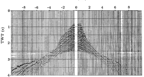
Fig. 14. Inline (X) horizontal component of OBS 10 after minimum phase predictive deconvolution (250 ms operator length, 50 pred. dist.) and bandpass filtering (5-18-35-71 Hz).
statics program. However, in this case there should be no shot statics as we have a marine source, and we have further-more only minor knowledge about the near surface of the sea bed. The fold of coverage in the shot and receiver domain is poor, and any static would also contain some error due to the approximations made in the geometry and positioning. As no shot/receiver domain residual statics can be calculated, CMP or CCP trim statics were attempted. The absence of any strong, consistent event to guide the correlation window produced erratic statics, and any improvements in the stacks were negligible.
The post stack processes used on the vertical component were also applied to the horizontal stacks. F-X deconvolu-tion removed random noise and increased the level of higher
frequencies, but the F-K filter degraded the stack, producing a rather smeared out section. Without a consistent event it was not possible to use horizon flattening, and even the sea bed (or direct arrival) was not coherent enough to be utilized. The final stacks were displayed with the same filter and scal-ing as for the vertical component; Figs. 16(a) and (b) show an example of CMP and CCP stacks with FX deconvolution. 3.5 Interpretation and modelling
E. BERGet al.: OBS-PROCESSING FOR LITHOLOGY AND FLUID PREDICTION 85
Fig. 15. Crossline (Y) horizontal component of OBS 10 after minimum phase predictive deconvolution (250 ms operator length, 50 pred. dist.) and bandpass filtering (5-18-35-71 Hz).
Fig. 16. Inline (X) horizontal component stack (pred. decon. 250/50 ms, 50 m CMP binning). a) CMP stack with FX deconvolution. b) CCP (Vp/Vs-ratio
of 2.5) stack with FX deconvolution.
of events and seismic patterns on the inline component. No wells are available for calibration or data correlation. The stackedVz-section can be considered as a P-wave section,
and correlates as expected well with the surface seismic data (Fig. 3). The top reservoir (Intra Campanian) and theflatspot anomaly are easily identified in these data sections. Also the structural features with dipping layers and the graben imme-diately west of the anomaly can be observed.
The processing and modelling of theVx component
sug-gested thatP-to-Sconverted reflections represent the domi-nant mode, and the detailed processing of this component fo-cused consequently on enhancingP-to-Sconversions. These results are consistent with recent synthetic modelling per-formed by Rodriguez-Suarezet al.(2000). The top reservoir reflector can be observed as thefirst strong dipping refl ec-tor at approximately 4500–5000 ms. Theflatspot anomaly can also be observed in the converted data, even though it is
not as clear as on theVz-section. The fact that the flatspot
can be (weakly) observed also forS-waves may suggest that the anomaly does not correspond to a purefluid contact, as this should normally cause absence of mode conversions at the anomaly. The presence of the anomaly in the horizontal stack might indicate diagenetic changes across thefluid con-tact, although it should be emphasized that density variations alone influids could cause mode conversions.
To support the interpretation and identify the most impor-tant P- andS-wave arrivals, ray-tracing was performed. A 2-D model for the OBS line was built from interpreted sur-face seismic data and RMS-velocity picks on CMP gathers.
ec-Fig. 17. Interpreted vertical component stack. The arrows on the enlarged part indicate the top of the reservoir and theflatspot, respectively.
tions forP-to-Pdata can be seen at 2.6 s and 2.7 s zero-offset traveltimes. These reflections could also be identified on the corresponding OBSVz-component.
P-to-S converted waves were modeled by varying the
Vp/Vs-ratio, and the modeled spikeograms were correlated
with the processed OBS inline component. After several iterations, a Vp/Vs-ratio of approximately 2.6±0.1 from
the sea-floor to the top of the reservoir provided reasonable traveltimefits between reflections on the modeled OBS data and interpreted reflections on the measured OBS data. The
S-velocity for the first two hundred meters below the sea
floor was assumed to be just below 200 m/s. The modelling thus indicated which measured reflections correspond to the target area. In the spikeogram in Fig. 19(b), P-to-S con-verted reflections from the target can be seen at zero-offset traveltimes at approximately 4.75 s and 4.9 s. The modeled zero-offset traveltimes are in reasonable agreement with the traveltimes observed on the processed inline section.
4.
Lithology and Fluid Prediction
From the interpreted Z and X component sections (Figs. 17 and 18) it is possible to measure the travel times within layers for both P- andS-waves, and hence calculate theVp/Vs-ratios for different intervals. IftS andtP are the
two way travel times measured between two horizons on the
X- andZ-sections, respectively, and one assumes that shear
Fig. 18. Interpreted inline horizontal component stack (CCP, same as Fig. 16(b)). The arrows on the enlarged part indicate the top of the reservoir and theflatspot, respectively.
waves are generated upon reflection, then;
VP VS
= tS−(tP/2)
(tP/2)
. (3)
The travel times were measured on the two sections by means of the“Screen Display”option in ProMAX and the horizons were picked (identically to the interpretation) with the picking tool. As the picks can be snapped to a peak, trough or zero crossing, all three were tried. As well as calculating a directVp/Vs-ratio over theflatspot (within the
assumed reservoir), the variation in theVp/Vs-ratio was
es-timated along the layer in which it is located. The results of the modelling and interpretation show a Vp/Vs-ratio of
approximately 2.6 in the overburden, which indicates partly unconsolidated shale, while theVp/Vs-ratio in the assumed
reservoir is approximately 1.8, which indicates more sand dominated facies. Outside theflatspot area within the same stratigraphic layers the Vp/Vs-ratio is estimated to be
ap-proximately 2.0. This indicates that hydrocarbons could be present in the assumed reservoir. The lower Vp/Vs-ratio
beneath the Intra Campanian unconformity, is also inferred from the modelling of the semi-regional OBS-data (Digranes
et al., 2000). It must be emphasized that the uncertainty in the Vp/Vs estimates, that mainly is related to uncertainties
interpreta-E. BERGet al.: OBS-PROCESSING FOR LITHOLOGY AND FLUID PREDICTION 87
Fig. 19. a) Model (interfaces) with ray-paths reflected from the target area. b) Traveltime curves (spikeogram) ofP-P- andP-S-reflections from the top of the reservoir and theflatspot.
tion concerning dating of interfaces, lithology andfluids has been confirmed, however, by recent drilling (the Norwegian Petroleum Directorat, unpublished information).
5.
Conclusions
The locally acquired OBS-data from the Vøring basin have been successfully processed by use of conventional reflection data processing methods, and stacked sections have been ob-tained both forP- andS-waves. The processing was difficult due to the irregular spatial sampling, limiting the pre-stack processing to trace-by-trace tools. A strong offset mute had to be applied to the vertical component due to the presence of strong multiples. These multiples were not present in the horizontal component data, and the application of the mute was hence not necessary for this component. The rotation of the horizontal components proved to be difficult, partly due to lower data quality for these components, and the quality of the stack (S-waves) was not as good as for the data from the vertical component (P-waves). Most of the processing effort was related to the geometry, velocity analysis and rotation of the horizontal components.
The frequency content (resolution) appears to be higher on the horizontal stack than on the corresponding stack from the vertical components. This difference can be contributed to the lowS-wave velocity in the interval from the sea-floor to the reservoir-level.
The data have been modeled by ray-tracing, and the
Vp/Vs-ratio was estimated to 2.6 from the sea-floor to the
top of the assumed reservoir, indicating domination of partly unconsolidated shale. TheVp/Vs-ratio within the reservoir
was estimated to 1.8, and within the same stratigraphic layers outside the area of theflatspot theVp/Vs-ratio was estimated
to 2.0. The lower ratio within the reservoir suggests that hy-drocarbons could be present.
The calculation of Vp/Vs-ratios presented in this study
are based on travel times from theP- andS-wave sections, which are far more robust and reliable than from conven-tional amplitude analysis. The results have been achieved by use of (only) one simple academic vessel and ocean bottom recorders primarily designed for the studies of earthquakes and regional seismic experiments. We believe that the study demonstrates the large potential more sophisticated experi-ments (geophone cables, clamped geophones etc.) have in
S-wave detection and reduction of risks in hydrocarbon ex-ploration.
exploration.
Furthermore, the acquisition and processing scheme devel-oped may also become important in scientific and commer-cial lithology andfluid predictions in settings like convergent margins.
Acknowledgments. We are indebted to Prof. M. A. Sellevoll at the Institute of Solid Earth Physics (IFJ), University of Bergen for his support during the planning of the experiment. The crew on R/V H˚akon Mosby is greatly acknowledged for their skills and help in all possible situations. We thank further the participating technicians and students from IFJ and the Hokkaido University. We also thank the Norwegian Petroleum Directorate for giving the permission for the experiment and to present part of the reflection profile VB-08-89, S. Vaage and Seres for modelling the air-gun configurations, Geoteam for processing the navigation data, Geco for providing air-chambers for the experiment, and Y. Li from the Hokkaido Uni-versity for a/d converting parts of the OBS-data. Finally, Statoil is thanked for the permission to present these results, and for econom-ical support.
Appendix A. Geometry Application
In ProMAX several methods can be used for creating the geometry necessary for processing and stacking the data, the simplest being a conventional marine 2D geometry created with the“Marine Geometry”tool. However, for this dataset there were several problems; the receivers were located at irregular intervals on the sea bed, they were stationary for the duration of the shooting, and the shots were not at regular intervals. The geometry was therefore more similar to a land 2D survey, but in order to create this type of geometry with the
“Geometry Spreadsheet”or “GMG Geoscribe (2D)”tools, shot coordinates would be needed. These problems were solved by manually generating the geometry by manipulation of trace headers, and then transfering this information from the headers back into ProMAX via the “Extract Database Files” tool. In order to further simplify the process, the source and receiver positions were reversed; the OBS stations were considered as shot points and the shot points as receiver locations. The geometry then appeared more regular to the database, and it is generally easier to work with common OBS gathers when they appear as shots orfieldfiles. The header words were created by re-sequencing headers and simple geometric calculations based on the trace co-ordinates. Each common OBS gather was re-numbered with a newfieldfile and the offset related headers were created by binning the offset header already present. The coordinates and surface locations were based on their distance from OBS location 1 and were assumed to be in a single vertical plane (2D). By calculating the distance to the OBS from OBS location 1 and adding 15000 m the sourcexcoordinate was created:
sou x =(obx x−415409)2−(obs y−7435151)2
+15000.
The traces in each OBS gather were given a receiver x
coordinate and a CMPxcoordinate by:
r ec x =sou s−o f f set
cmp x =sou x−r ec x
2 .
Note that the associatedycoordinates were set to 0.0. The surface shot point locations were calculated in a similar way,
by reference to SP3627 at OBS location 1:
sou sloc=3627+I N T
In the normal mid-point sense, cmp xcan be considered as a point along a CMP line for each trace and can therefore be binned into intervals. Various intervals (from 25 m to 200 m) were tested, and a bin width of 50 m proved to be adequate. The average fold for this bin width, if all offsets are included in the stack, is around 80 and the number of CMP bins is 338, as can be seen in Fig. 7. Discarding traces not contributing to the stack at the target level leaves a fold of stack of around 25. For asymmetric or common conversion point binning of the horizontal components, the calculation of CCPx includes constants derived from theVp/Vs-ratio.
The CCP formula used is:
When theVp/Vs-ratio equals one, this equation gives
nor-mal CMP numbering. A geometry was created for the hori-zontal component data with aVp/Vs-ratio of 1.0, 1.75, 2.0,
2.5 and 2.75. As the processing software expects data to have a common mid or depth point number stored as the header word CDP, each dataset that has a geometry applied to it must copy either the CCP or the CMP information into the CDP family of headers. This step was best performed when the“master”dataset was read (the headers only) and the“Extract Geom Files”tool was used. The master dataset was then copied into the work area, and the new geometry was loaded into the trace headers.
Appendix B. Rotation of the Horizontal
Compo-nents
As there was no compass within the instruments, the orien-tation of the two horizontal components was unknown, and attempts were thus made to rotate the components into in-line (X) and crossline (Y) components. This was performed on the raw-data, and after application of a 250 ms operator and 50 ms gap predictive deconvolution (the same as for the vertical component), as the data were contaminated by low frequency ringing. Figure 6 shows one of the horizontal com-ponents of OBS 10 s without any processing. Application of the deconvolution and band passfiltering provide a marked improvement and allows many higher frequency events to be distinguished (Fig. 14).
E. BERGet al.: OBS-PROCESSING FOR LITHOLOGY AND FLUID PREDICTION 89
Two sets of software were used for this purpose (Sensor Geo-physical and ProMAX VSP), both depending strongly on a defined time window having a clean wavelet (afirst arrival) to operate on. The Sensor Geophysical software was the simplest to use and outputs a display showing a time lag (for anisotropy) and rotation angle (either positive or negative). However, when the angle (including the polarity) was used to rotate the data the components did not show the expected energy transfer and the results were thus unsuccessful. This could be due to the fact that this software is primarily de-signed to detect anisotropy characteristics of the data.
The ProMAX VSP software was more difficult to apply as it is designed for data recorded in boreholes, but with some manipulation of the geometry it was possible to use the
“3-Component Reorientation”tool. The output is given as a rotation angle for each trace, and it is then possible to average these visually (by transfering them to the ProMAX database) or to use the trace manipulation processes to average them as header values.
As the rotation of the data was not conclusive and did not appear satisfactory for all of the OBSs, both methods were used. Firstly, it was assumed that the component with the maximum energy (i.e. largest RMS level) is the X compo-nent (Fig. 14) and the compocompo-nent with the minimum energy is theY component (Fig. 15), and secondly, the components were rotated with the angles found. These twoXcomponent datasets were then processed further with conventional pro-cessing tools. It is important to underline that the true inline direction was not needed, as most of the analyzes was based on traveltime information.
References
Caldwell, J., Marine multicomponent seismology,The Leading Edge, Nov., 1274–1282, 1999.
Christensen, N. I., Pore pressure and oceanic crustal seismic structure, Geo-phys. J. R. Astron. Soc.,79, 411–423, 1984.
Christensen, N. I. and D. M. Fountain, Constitution of the lower continental crust based on experimental studies of seismic velocities in granulite, Geol. Soc. Am. Bull.,86, 227–236, 1975.
Crampin, S., The scattering of S waves in the crust,Pure and Applied Geophysics,132, 67–91, 1990.
Digranes, P., R. Mjelde, S. Kodaira, H. Shimamura, T. Kanazawa, H.
Shiobara, and E. W. Berg, Modelling shear waves in OBS data from the Vøring basin (Northern Norway) by 2-D ray-tracing,Pure and Applied Geophysics,4, 611–629, 1996.
Digranes, P., R. Mjelde, S. Kodaira, H. Shimamura, T. Kanazawa, H. Shiobara, and E. W. Berg, Comparison between a regional and semi-regional S-wave model from OBS data in the Vøring basin, N. Norway, Pure and Applied Geophysics, 2000 (submitted).
Kanazawa, T., Technical description of TK92-type ocean bottom seismome-ter, inInvestigation of the Central and Northern Part of the Vøring Basin by Use of Ocean Bottom Seismographs, R/V H˚akon Mosby 22 Aug.–24 Sept. 1992, Cruise Report, edited by R. Mjeldeet al., 87 pp., Statoil report, 1993.
Kern, H., Elastic wave velocity in crustal and mantle rocks at high pressure and temperature: The role of high-low quartz transition and of dehydra-tion reacdehydra-tions,Phys. Earth Planet. Inter.,29, 12–23, 1982.
Mjelde, R., E. W. Berg, A. Strøm, O. Riise, H. Shimamura, T. Kanazawa, H. Shiobara, S. Kodaira, and J. P. Fjellanger, An extensive Ocean Bottom Seismograph survey in the Vøring basin, N. Norway,First Break,14, 247–256, 1996.
Mjelde, R., S. Kodaira, H. Shimamura, T. Kanazawa, H. Shiobara, E. W. Berg, and O. Riise, Crustal structure of the central part of the Vøring basin, N. Norway, from three-component ocean bottom seismographs, Tectonophys.,277, 235–257, 1997a.
Mjelde, R., S. Kodaira, P. Digranes, H. Shimamura, T. Kanazawa, H. Shiobara, and E. W. Berg, Comparison between a regional and semi-regional crustal OBS-model in the Vøring basin, N. Norway,Pure and Applied Geophysics,149, 641–665, 1997b.
Neidell, N. S., Land applications of S waves,Geophysics: The Leading Edge of Exploration, 32–44, 1985.
Nur, A. and G. Simmons, The effect of saturation on velocity in low porosity rocks,Earth Planet. Sci. Lett.,7, 183–193, 1969.
Rodriguez-Suarez, C., R. R. Stewart, and G. F. Margrave, Where does S-wave energy on OBC recordings come from?, 70th Ann. Intl. SEG Meet-ing, Extended abstract, 2000.
Shimamura, H., OBS technical description, inSeismiske Undersøkelser av Lofoten Marginen og Refleksjonsseismiske Test-m˚alinger p˚a Mohns Rygg, M/S H˚akon Mosby, 29 Juli–19 August, 1988, Cruise Report, edited by M. A. Sellevoll, 72 pp., Inst. of Solid Earth Physics Report, Univ. of Bergen, 1988.
Shiobara, H., A. Nakanishi, R. Mjelde, T. Kanazawa, E. W. Berg, and H. Shimamura, Precise determination of OBS positions by using acoustic transponders and CTD,Marine Geophysical Researches,19, 199–209, 1997.
Spencer, J. W. and A. Nur, The effect of pressure, temperature and pore water on velocities in Westerly granite,J. Geophys. Res.,81, 899–904, 1976.