Multi-hadron-state contamination in nucleon observables from
chiral perturbation theory
?OliverBär1
1Institut für Physik, Humboldt Universität zu Berlin, Newtonstraße 15, D-12489 Berlin, Germany
Abstract.Multi-particle states with additional pions are expected to be a non-negligible source of the excited-state contamination in lattice simulations at the physical point. It is shown that baryon chiral perturbation theory (ChPT) can be employed to calculate the contamination due to two-particle nucleon-pion states in various nucleon observables. Results to leading order are presented for the nucleon axial, tensor and scalar charge and three Mellin moments of parton distribution functions: the average quark momentum fraction, the helicity and the transversity moment. Taking into account experimental and phenomenological results for the charges and moments the impact of the nucleon-pion-states on lattice estimates for these observables can be estimated. The nucleon-pion-state contribution leads to an overestimation of all charges and moments obtained with the plateau method. The overestimation is at the 5-10% level for source-sink separations of about 2 fm. Existing lattice data is not in conflict with the ChPT predictions, but the comparison suggests that significantly larger source-sink separations are needed to compute the charges and moments with few-percent precision.
1 Introduction
Chiral perturbation theory (ChPT) is a frequently used tool in the analysis of Lattice Quantum Chro-modynamics (QCD) data. Well-known examples are the calculation of finite-volume (FV) e↵ects
or the light quark mass dependence of physical observables. ChPT results for the quark mass de-pendence are commonly used in the chiral extrapolation to relate unphysical lattice results obtained at heavy quark masses to the physical point with quark masses as light as in nature. However, the need for a chiral extrapolation has been slowly fading away. Constant progress in computer power as well as advances in simulation algorithms have made lattice simulations possible with the light quark masses set to their physical values. Suchphysical point simulationseliminate altogether the systematic uncertainties associated with a chiral extrapolation.
In this talk I briefly report on a di↵erent application of ChPT to Lattice QCD, namely the study
of excited-state contaminations. In physical point simulations one can expect multi-particle states with additional light pions to become a non-negligible excited-state contamination in many correla-tion funccorrela-tions measured on the lattice. The calculacorrela-tion of nucleon structure observables is a familiar example where the excited-state contamination is known to be a source of significant systematic uncer-tainty. The multi-particle states expected to be most relevant in this case are two-particle nucleon-pion (N⇡) states, and their contribution is accessible by ChPT.
?Talk given at the 35th International Symposium on Lattice Field Theory, 18 - 24 June 2017, Granada, Spain.
2
N
⇡
-state contribution in nucleon correlation function
Let us start with a simple but illustrative example, the nucleon 2pt functionG2pt(t)=X
~ x
hN(~x,t)N(0,0)i, (1)
which is measured in Lattice QCD to compute the nucleon mass. N,N denote interpolating fields with the quantum numbers of the nucleon. The sum over the finite spatial volumeV = L3 projects
to vanishing spatial momentum. Performing the standard spectral decomposition the 2pt function is found to be given by a sum of exponentials,
G2pt(t)=c0e−MNt+c1e−E1t+c2e−E2t+. . . , (2)
wheret>0 and the orderingMN <E1 <E2 < . . .for the energies is assumed. By construction, the first exponential contains the nucleon mass. The coefficientc0associated with it is the squared matrix
element of the interpolating field between the vacuum and the nucleon at rest. The other terms stem from excited states with the same quantum numbers as the nucleon, and the coefficientscjinvolve the matrix elements with the excited states instead of the nucleon state.
In lattice simulations one usually computes the e↵ective nucleon mass, defined as the negative
time derivative of lnG2pt(t). With (2) we obtain (∆Ek=Ek−MN)
MN,e↵ =MN+c1
c0∆E1e
−∆E1t+c2
c0∆E2e
−∆E2t+. . . . (3)
In the limitt! 1the e↵ective mass converges to the nucleon mass. For large but finitetthere is an
excited-state contamination present. Although exponentially suppressed the euclidean time separation needs to be sufficiently large for the excited-state contamination to be small. In practice the
signal-to-noise problem [1,2] prevents us from going to very large euclidean time separations to make the excited-state contribution arbitrarily small. The smaller the pion mass the shorter the time separation for which the e↵ective mass can be measured with small statistical errors. Typical time separations at
present are between 1 to 1.5 fm.
2
N⇡
-state contribution in nucleon correlation function
Let us start with a simple but illustrative example, the nucleon 2pt function
G2pt(t)=X
~ x
hN(~x,t)N(0,0)i, (1)
which is measured in Lattice QCD to compute the nucleon mass. N,N denote interpolating fields with the quantum numbers of the nucleon. The sum over the finite spatial volumeV = L3projects
to vanishing spatial momentum. Performing the standard spectral decomposition the 2pt function is found to be given by a sum of exponentials,
G2pt(t)=c0e−MNt+c1e−E1t+c2e−E2t+. . . , (2)
wheret >0 and the orderingMN <E1 <E2 < . . .for the energies is assumed. By construction, the first exponential contains the nucleon mass. The coefficientc0associated with it is the squared matrix
element of the interpolating field between the vacuum and the nucleon at rest. The other terms stem from excited states with the same quantum numbers as the nucleon, and the coefficientscjinvolve the matrix elements with the excited states instead of the nucleon state.
In lattice simulations one usually computes the e↵ective nucleon mass, defined as the negative
time derivative of lnG2pt(t). With (2) we obtain (∆Ek=Ek−MN)
MN,e↵ =MN+c1
c0∆E1e
−∆E1t+c2
c0∆E2e
−∆E2t+. . . . (3)
In the limitt! 1the e↵ective mass converges to the nucleon mass. For large but finitetthere is an
excited-state contamination present. Although exponentially suppressed the euclidean time separation needs to be sufficiently large for the excited-state contamination to be small. In practice the
signal-to-noise problem [1,2] prevents us from going to very large euclidean time separations to make the excited-state contribution arbitrarily small. The smaller the pion mass the shorter the time separation for which the e↵ective mass can be measured with small statistical errors. Typical time separations at
present are between 1 to 1.5 fm.
From experiment we can get some idea about the states that contribute to the 2pt function in a finite spatial volume. There is a contribution from resonance states that are associated to the nucleon resonances in infinite volume, the most prominent one being the Roper resonanceN⇤(1440).1 In addition there is the contribution from multi-particle states, e.g. 2-particleN⇡states, 3-particleN⇡⇡ states etc. The multi-particle-state contribution is expected to become rapidly relevant for pion masses approaching the physical value. This is easily seen by ignoring the interaction energy of the particles, which is expected to be rather small since the pions interact only weakly with the nucleon and with themselves. Within this approximation the energy of the N⇡⇡state with all three particles at rest is equal to MN+2M⇡ ⇡ 1.3MN. For a two-particleN⇡state to contribute both nucleon and pion need non-vanishing and opposite spatial momenta. If we assume periodic boundary conditions for the finite spatial volume the spatial momenta are discrete,~pk=2⇡~k/L, with~khaving integer-valued components. The larger the lattice extentLthe smaller the discrete energies of theN⇡states allowed by the boundary conditions. If we assume the typical valueM⇡L = 4 we find threeN⇡states with an energy less than MN⇤ ⇡ 1.5MN (see fig.1). This number increases to seven for M⇡L = 6, as realized in the simulations of the PACS collaboration [4]. At this conference Y. Kuramashi reported
1The precise relation between infinite volume resonance properties and the finite volume energy spectrum has been worked out first in Ref. [3].
Sketch: MN MN 1.5MN
Excited states in the nucleon sector
Excited states contributing to the nucleon 2-pt function: Resonances: Ν*(1440), Ν*(1710), …
Nucleon-pion states: Νπ, Νππ, …
Multi-particle states become important for physical pion masses
MN+ 2M 1.3MN
ignore interaction
M ,physL= 4 #N(pk)π( pk) = 3
Finite volume, periodic bc ⇒ discrete momenta
pk=
2π Lk
M ,physL= 6 #N(pk)π( pk) = 7
Figure 1.Sketch of the energies of the lowestN⇡states (diamonds) that contribute to the nucleon 2pt function. Discrete momenta corresponding toM⇡L = 4 (orange) andM⇡L =6 (purple) are considered and interaction energies are ignored. The blue square represents the energy of theN⇡⇡state with all three particles at rest.
on simulations on even larger lattices withM⇡L ⇡ 7.7 [5], and such volumes imply ten N⇡states with energy below 1.5MN. The main conclusion is that quite a few multi-particle states are expected to contribute to the sum in eq. (2) before a contribution of the first resonance state appears. Thus, in physical point simulations the multi-particle states dominate the excited-state contamination in the asymptotic regime of large but still finitet.
The impact of the multi-particle states to the 2pt function depends also on the size of the coef-ficientscj,j ≥ 1. Not much is known a priori about these coefficients, except for the fact that a
coefficient associated with ann-particle state is, in a finite spatial volume, suppressed by (1/L3)n−1. Note that this volume suppression cannot be taken as an argument for a small multi-particle-state con-tribution ifLis large. Although the contribution of each individual multi-particle state decreases, more and more states contribute the larger the volume is. In particular, the multi-particle-state contribution is not a FV e↵ect and will not disappear in the infinite-volume limit.
Other observables than the nucleon mass are expected to be even more a✏icted by an excited state
contamination. Still rather straightforward to compute numerically are nucleon charges and Mellin moments of parton distribution functions. All these observables refer to nucleon matrix elements hN(~p)|OX|N(~p)iof a local quark bilinearOXbetween nucleon states and with zero momentum transfer. In case of the standard axial vector current as well as the tensor and scalar density forOX(X=A,T,S) one obtains the axial, tensor and scalar chargesgA, gT andgS.2 The axial charge is known at the per mille level from neutron beta decay [6] and considered to be a benchmark observable for lattice QCD. The scalar and tensor charge are only poorly known, but enjoy a revived interest. New nuclear beta-decay experiments aim at an order of magnitude more precise upper bounds for these charges. In order to constrain beyond-standard-model physics lattice QCD estimates for these charges with 10-15% uncertainties will be needed [7].
Parton distribution functions (pdfs) are difficult to access directly in Euclidean space-time. Instead,
one can define and calculate Mellin moments that can be related to matrix elements of local one-derivative operators. For example, the average quark momentum fractionhxiu−d (also called the first unpolarized moment) involves the operatorVµ⌫ = uγ{µD−⌫}u−dγ{µD−⌫}d with the (color covariant) derivative given byD−
µ =(!−Dµ−D−µ)/2, and the curly brackets refer to symmetrization with respect to the indicesµ, ⌫ and subtraction of the trace. The helicity momenthxi∆u−∆d and the transversity momenthxiδu−δdare defined analogously and di↵er in the gamma matrices involved. Pdf moments are accessible phenomenologically and some of them have been determined with percent accuracy. For example, in Ref. [8] the average quark momentum fraction is found ashxiu−d,phen=0.1655(39) (in the MS scheme at 2 GeV).
2Throughout I will exclusively refer to the flavor nonsinglet charges.
The standard methods to compute the charges and moments require the computation of the 3pt function.3 To be specific, we need the 3pt function
G3pt,A(t,t0)= X
~ x,~y
Γ0k,↵βhNβ(~x,t)Ak3(~y,t0)N↵(~0,0)i (4)
in case of the axial charge. The nucleon interpolating fields are the same as in the 2pt function. A spatial component of the non-singlet axial vector current is placed at some operator insertion timet0 between source and sink, and the projectorΓ0kis chosen such that the leading part of the 3pt function
is proportional togA. Forming the ratio with the 2pt function,
RA(t,t0)=G3pt,A(t ,t0)
G2pt(t) , (5)
and performing the spectral decomposition of both numerator and denominator one finds the repre-sentation
RA(t,t0)=gA+bA,1e−∆E1(t−t0)+b˜A,1e−∆E1t0+c˜A,1e−∆E1t+. . . (6) for the ratio. In the limit that all timest,t0andt−t0go to infinity the ratio tends to a constant, the axial charge. For finite times there are again excited-state contributions present stemming from resonance and multi-hadron states. The coefficientsbA,1,b˜A,1,c˜A,1in (6) are ratios of matrix elements involving the axial vector current as well as the interpolating fields and the states for the vacuum, the nucleon at rest and the first excited state.
The excited-state contributions in eq. (6) involves the three time separationst−t0,t0 andt. As already mentioned, the source-sink separationstaccessible in numerical simulations are limited due to the signal-to-noise problem. Sincet−t0andt0are even smaller thantwe anticipate a significantly larger excited-state contamination in calculations of the axial charge (as well as the other charges and the pdf moments). For large time separations, however, we expect the multi-hadron states to be the dominant source for the excited-state contribution, since these have the smallest gap to the energy of the single nucleon state.
Topic of this talk is that the correlation function ratios can be computed in ChPT. Such calculations provide the coefficientsbA,j,b˜A,j,c˜A,jin (6) associated with multi-particle-state contributions. Results are available for the two-particleN⇡contribution in the ratios for the three nucleon charges and the three pdf moments introduced before [10–12]. For a recent review see Ref. [13]. Calculations for contributions of theN⇡⇡and∆⇡states will be analogous but have not been performed yet.
That BChPT can be employed to compute the multi-particle state contribution in correlation func-tions is neither surprising nor a new idea [14,15]. In fact, Brian Tiburzi [14] was probably the first to compute theN⇡-state contribution toRA in an attempt to explain, at least qualitatively, why most lattice results at the time underestimated the experimental value of the nucleon axial charge. However, theN⇡-state contribution is found to lead to an overestimation of the axial charge and the idea did not receive much attention.
In the following I will present results for the nucleon axial, tensor and scalar charges and the three pdf moments introduced before. The calculation di↵ers in some details from the early one in Ref.
[14]. The discreteness of the nucleon and pion momenta due to a finite spatial volume is taken into account. In addition, the mapping of smeared nucleon interpolating fields, commonly used in lattice calculations, to ChPT has been put on firmer grounds [16,17]. More importantly, having results for six instead of only one observable we find theN⇡-state contribution in all six observables to be related. This is nothing but chiral symmetry at work.
The standard methods to compute the charges and moments require the computation of the 3pt function.3 To be specific, we need the 3pt function
G3pt,A(t,t0)= X
~x,~y
Γ0k,↵βhNβ(~x,t)Ak3(~y,t0)N↵(~0,0)i (4)
in case of the axial charge. The nucleon interpolating fields are the same as in the 2pt function. A spatial component of the non-singlet axial vector current is placed at some operator insertion timet0 between source and sink, and the projectorΓ0kis chosen such that the leading part of the 3pt function
is proportional togA. Forming the ratio with the 2pt function,
RA(t,t0)=G3pt,A(t ,t0)
G2pt(t) , (5)
and performing the spectral decomposition of both numerator and denominator one finds the repre-sentation
RA(t,t0)=gA+bA,1e−∆E1(t−t0)+b˜A,1e−∆E1t0+c˜A,1e−∆E1t+. . . (6) for the ratio. In the limit that all timest,t0andt−t0go to infinity the ratio tends to a constant, the axial charge. For finite times there are again excited-state contributions present stemming from resonance and multi-hadron states. The coefficientsbA,1,b˜A,1,c˜A,1in (6) are ratios of matrix elements involving the axial vector current as well as the interpolating fields and the states for the vacuum, the nucleon at rest and the first excited state.
The excited-state contributions in eq. (6) involves the three time separationst−t0,t0 andt. As already mentioned, the source-sink separationstaccessible in numerical simulations are limited due to the signal-to-noise problem. Sincet−t0andt0are even smaller thantwe anticipate a significantly larger excited-state contamination in calculations of the axial charge (as well as the other charges and the pdf moments). For large time separations, however, we expect the multi-hadron states to be the dominant source for the excited-state contribution, since these have the smallest gap to the energy of the single nucleon state.
Topic of this talk is that the correlation function ratios can be computed in ChPT. Such calculations provide the coefficientsbA,j,b˜A,j,c˜A,jin (6) associated with multi-particle-state contributions. Results are available for the two-particleN⇡contribution in the ratios for the three nucleon charges and the three pdf moments introduced before [10–12]. For a recent review see Ref. [13]. Calculations for contributions of theN⇡⇡and∆⇡states will be analogous but have not been performed yet.
That BChPT can be employed to compute the multi-particle state contribution in correlation func-tions is neither surprising nor a new idea [14,15]. In fact, Brian Tiburzi [14] was probably the first to compute theN⇡-state contribution toRAin an attempt to explain, at least qualitatively, why most lattice results at the time underestimated the experimental value of the nucleon axial charge. However, theN⇡-state contribution is found to lead to an overestimation of the axial charge and the idea did not receive much attention.
In the following I will present results for the nucleon axial, tensor and scalar charges and the three pdf moments introduced before. The calculation di↵ers in some details from the early one in Ref.
[14]. The discreteness of the nucleon and pion momenta due to a finite spatial volume is taken into account. In addition, the mapping of smeared nucleon interpolating fields, commonly used in lattice calculations, to ChPT has been put on firmer grounds [16,17]. More importantly, having results for six instead of only one observable we find theN⇡-state contribution in all six observables to be related. This is nothing but chiral symmetry at work.
3The recently proposed method [9] inspired by the Feynman-Hellman theorem avoids the explicit calculation of the 3pt function.
3 The correlation functions in ChPT
Chiral perturbation theory refers to the low-energy e↵ective theory of QCD based on spontaneous
chiral symmetry breaking [18–20]. It has been around for many years and there seems no need to introduce or review it here.4
The two most prominent applications in Lattice QCD are the calculation of the quark mass depen-dence of observables and FV e↵ects due to the pions. Starting point for the application we have in
mind here, the excited-state contribution caused by two-particleN⇡states, is the same well-established formulation of Baryon ChPT (BChPT) [29,30] that is basis for the other applications as well. We work to leading order only, thus we do not encounter any of the subtleties associated with the loop expansion in BChPT. We consider SU(2) BChPT and assume isospin symmetry. In this case the chi-ral e↵ective theory contains the three mass degenerate pions⇡aand the nucleon doublet =(p,n)T involving the mass degenerate proton and neutron fields. The interaction term relevant here is given by5
Lint,1⇡ =i
gA
2f γµγ5σa @µ⇡a, (7)
which implies the well-known one-pion-exchange-potential (OPEP) between a nucleon pair. It is proportional to the ratiogA/f of two LO low-energy coefficients (LECs), the chiral limit values of the axial charge and the pion decay constant.
The e↵ective operators for the axial vector current and the scalar density have been known for a
long time [29,31]. The operators needed for the average quark momentum fraction and the helicity moment too can be taken from the literature [32,33]. The expressions associated to the tensor op-erators, needed for the tensor charge and the transversity moment, have been derived following the general procedure described in Ref. [31]. The explicit expressions are not displayed here but can be found in Refs. [11,12]. Still, it is worth pointing out that the chiral limit values of all charges and pdf moments we are interested in appear as LECs in these e↵ective operators. These are input parameters
of ChPT.
The chiral expressions for the nucleon interpolating fields are also needed. These too are derived based on the transformation properties under chiral symmetry and parity [34]. The standard local 3-quark baryon operators [35,36] have been mapped to ChPT in Ref. [37]. Smeared interpolating fields are mapped to the same pointlike expressions but with di↵erent LECs provided the smeared quark
fields transform as their local analogues under parity and chiral symmetry. This, for instance, is the case in Gaussian and exponential smearing [38–40] or the gradient flow [41]. However, the smearing radius must be small compared to the Compton wavelength of the pion, i.e.Rsmear ⌧1/M⇡[16,17]. For physical pion masses this inequality seems reasonably well satisfied for smearing radii up to a few tenths of a fermi.
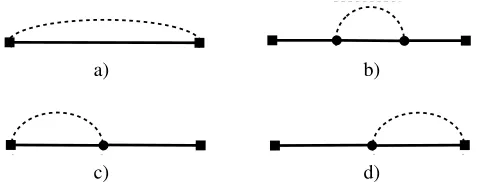
With these elements the calculation of the 2pt and 3pt functions is a standard perturbative calcula-tion in ChPT. It seems convenient to use the time-momentum representacalcula-tion for the pion and nucleon propagators since it directly yields the time dependence of the correlation functions. Figure2shows the leading diagrams with anN⇡-state contribution to the 2pt function. These diagrams contain a con-tribution that drops o↵exponentially with the total energyEN⇡,n=EN,n+E⇡,nof a nucleon-pion state, where the discrete spatial momenta are back-to-back,~pN,n =−~p⇡,n. We are interested in the prefactor of this exponential. Note that even though the diagrams in fig.2are 1-loop diagrams the calculation of theN⇡-state contribution does not involve a summation over some undetermined momentum, i.e.
4There exist numerous reviews and lecture notes on ChPT that di↵er in scope and length, e.g. Refs. [21–27]. A particularly useful review of Baryon ChPT that also covers applications to lattice QCD is given in Ref. [28].
5We work in Euclidean space time.
a) b)
c) d)
Figure 2.Feynman diagrams for the nucleon 2pt function. The squares represent the nucleon interpolating fields at timestand 0. The circles represent a vertex insertion at an intermediate space-time point; and an integra-tion over this point is implicitly assumed. The solid and dashed lines represent nucleon and pion propagators, respectively.
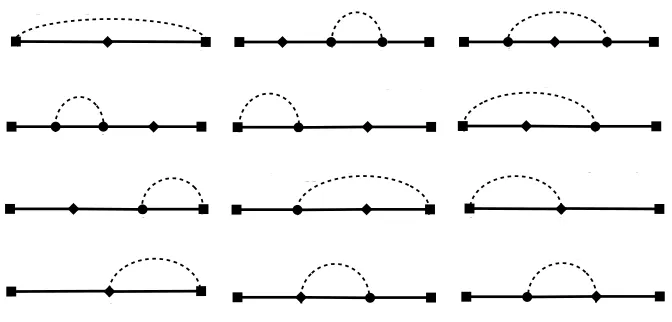
it is a tree-level calculation.6 Figure3shows the leading diagrams with an N⇡-state contribution to the 3pt functions.
The calculation of the Feynman diagrams is straightforward. The result for the ratio of the 3pt and 2pt functions is of the general form
RX(t,t0)=gXh1+X
~pn ⇣
bX,ne−∆En(t−t0)+b˜X,ne−∆Ent0+c˜X,ne−∆Ent⌘i (8)
for all three nucleon charges (X = A,T,S), with∆En =EN⇡,n−MN. An analogous result is found for the moments. The non-trivial results of the calculation are the coefficientsbX,n,b˜X,n,c˜X,nin all six ratios. The exact expressions for these coefficients can be found in Refs. [11,12] and are not displayed
here. Still, it is noteworthy that all coefficients involve a product of two universal factors, for example
˜
cX,n= 1 16(f L)2E
⇡,nL 1−
MN
EN,n !
. . .
!
. (9)
The first factor on the right hand side shows the anticipated volume suppression factor 1/L3of a two-particle state in a finite spatial volume. It combines with the pion decay constant and the pion energy to the dimensionless combination 1/(f L)2E
⇡,nL. The second factor (1−MN/EN,n) vanishes if the momentum of the nucleon (and the pion) is zero. This has to be the case since the nucleon-pion state with both particles at rest does not contribute to the correlation function because it is parity odd. The remaining factor is non-universal and not very illuminating.
More interesting than the exact expressions is the fact that the coefficients do not depend on the
LECs associated with the nucleon interpolating fields. To LO these cancel in the ratioRX. Conse-quently, the LON⇡-state contribution to the ratios is the same for pointlike and for smeared interpo-lating fields, since the di↵erence between these interpolators is encoded in their di↵erent values for
the LECs. However, this universality property will be lost at higher orders in the chiral expansion. The coefficients depend on a few parameters only: The pion mass and pion decay constant, the
finite volume viaM⇡L and four more LECs (the chiral limit values of the nucleon mass, the axial charge, the average quark momentum fraction and the helicity moment). All these parameters can be estimated using their experimental or phenomenological values. With this input we can estimate the
N⇡-state contribution to the ratios calculated in lattice simulations.
6Diagrams b) - d) also contain single-nucleon contributions dropping o↵with exp(−MNt), and this contribution does involve a sum over all momenta of the intermediateN⇡pair. Diagram b), for instance, is essentially the nucleon self-energy diagram that leads to the well-knownM3
a) b)
c) d)
Figure 2.Feynman diagrams for the nucleon 2pt function. The squares represent the nucleon interpolating fields at timestand 0. The circles represent a vertex insertion at an intermediate space-time point; and an integra-tion over this point is implicitly assumed. The solid and dashed lines represent nucleon and pion propagators, respectively.
it is a tree-level calculation.6 Figure3shows the leading diagrams with anN⇡-state contribution to the 3pt functions.
The calculation of the Feynman diagrams is straightforward. The result for the ratio of the 3pt and 2pt functions is of the general form
RX(t,t0)=gXh1+X
~ pn
⇣
bX,ne−∆En(t−t0)+b˜X,ne−∆Ent0+c˜X,ne−∆Ent⌘i (8)
for all three nucleon charges (X =A,T,S), with∆En =EN⇡,n−MN. An analogous result is found for the moments. The non-trivial results of the calculation are the coefficientsbX,n,b˜X,n,c˜X,nin all six ratios. The exact expressions for these coefficients can be found in Refs. [11,12] and are not displayed
here. Still, it is noteworthy that all coefficients involve a product of two universal factors, for example
˜
cX,n= 1 16(f L)2E
⇡,nL 1−
MN
EN,n !
. . .
!
. (9)
The first factor on the right hand side shows the anticipated volume suppression factor 1/L3of a two-particle state in a finite spatial volume. It combines with the pion decay constant and the pion energy to the dimensionless combination 1/(f L)2E
⇡,nL. The second factor (1−MN/EN,n) vanishes if the momentum of the nucleon (and the pion) is zero. This has to be the case since the nucleon-pion state with both particles at rest does not contribute to the correlation function because it is parity odd. The remaining factor is non-universal and not very illuminating.
More interesting than the exact expressions is the fact that the coefficients do not depend on the
LECs associated with the nucleon interpolating fields. To LO these cancel in the ratioRX. Conse-quently, the LON⇡-state contribution to the ratios is the same for pointlike and for smeared interpo-lating fields, since the di↵erence between these interpolators is encoded in their di↵erent values for
the LECs. However, this universality property will be lost at higher orders in the chiral expansion. The coefficients depend on a few parameters only: The pion mass and pion decay constant, the
finite volume via M⇡Land four more LECs (the chiral limit values of the nucleon mass, the axial charge, the average quark momentum fraction and the helicity moment). All these parameters can be estimated using their experimental or phenomenological values. With this input we can estimate the
N⇡-state contribution to the ratios calculated in lattice simulations.
6Diagrams b) - d) also contain single-nucleon contributions dropping o↵with exp(−MNt), and this contribution does involve a sum over all momenta of the intermediateN⇡pair. Diagram b), for instance, is essentially the nucleon self-energy diagram that leads to the well-knownM3
⇡term in the 1-loop ChPT result for the nucleon mass [29].
Figure 3.Feynman diagrams for the LO nucleon-pion contribution in the 3pt functions. The diamond stands for the operator insertion at timet0.
4 Impact on lattice calculations
The simplest estimator for the charges and pdf moments is the so-called midpoint estimate. It is based on a simple observation: For a given source-sink separationtthe excited-state contribution toRX is minimized if the operator insertion timet0is in the middle between source and sink. Therefore, the best estimate for the charges and moments is the midpoint valueRX(t,t/2). It is essentially equivalent to what is called plateau estimate, and we will use this terminology in the following.
The experimental/phenomenological values for the masses and LECs can be found in the literature
[6,8,42].7With these input parameters being fixed the LO ChPT result forN⇡-state contribution is a function of the spatial volume only.
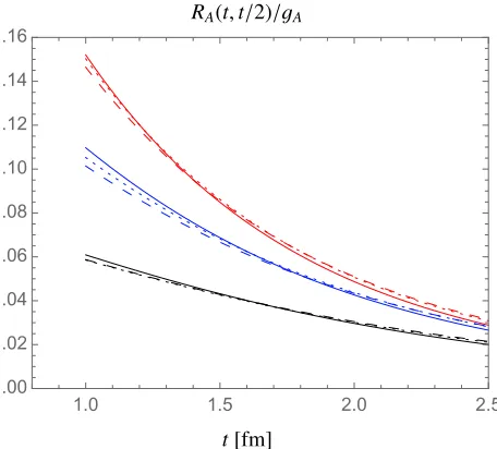
Fig.4shows the plateau estimategA,plat(t) ⌘ RA(t,t/2) for the axial charge divided by gA as a function of the source-sink separationt. Without the excited-state contribution this ratio would be equal to 1. Any deviation from this constant value shows directly theN⇡contribution to the plateau estimate in percent. Results are shown for three di↵erent lattice sizes with M⇡ = 4,5 and 6 (solid, dotted and dashed lines). Di↵erent colors refer to di↵erent numbers ofN⇡states taken into account in the sum over the discrete spatial momenta~pn, cf. equation (8). For the black linesN⇡states with a total energy up about 1.35 GeV are included. The blue and red lines correspond to total energies up to about 1.6 and 1.9 GeV. Note that the number of states corresponding to these energies depends on the spatial lattice extentL. For example, the black lines in fig.4correspond to 2, 3 and 5 states for
M⇡L=4,5 and 6, respectively.
Apparently, the di↵erences between lines of the same color are very small, i.e. theN⇡contribution is essentially the same for the three di↵erentM⇡Lvalues displayed in the figure. As already mentioned in the introduction, the 1/L3suppression of the two-particle-state matrix elements is expected to be largely compensated by a growing number ofN⇡states in a given energy interval. Still, it is perhaps somewhat surprising that the di↵erences between the three di↵erent volumes are so small.
7For the results presented here the following simplified values have been used:M⇡=140 MeV,MN=940 MeV,gA=1.27, f⇡ =93 MeV,hxiu−d =0.165 andhxi∆u−∆d =0.19. Errors in these estimates are ignored since they are too small to be significant for the LO ChPT results.
RA(t,t/2)/gA
1.0 1.5 2.0 2.5
1.00 1.02 1.04 1.06 1.08 1.10 1.12 1.14 1.16
t[fm]
Figure 4.The plateau estimateRA(t,t/2) normalized bygAas a function of the source-sink separationt. Results
are shown forM⇡L = 4 (solid lines), M⇡L =5 (dotted lines) and M⇡L = 6 (dashed lines). Di↵erent colors
distinguish between three di↵erent upper energy bounds for theN⇡states taken into account (see main text).
Fig.4also shows that theN⇡contribution leads to an overestimation of the axial charge by the plateau estimate. Before reading o↵a number from the plot recall that ChPT is an expansion in
small pion momenta. We may expect reasonably reliable ChPT results for the low-momentumN⇡ states, depicted by the black lines in the plot. The chiral expansion of the high-momentumN⇡states, included in the blue and red curves, is expected to work less well if it works at all.
This restriction implies that the source-sink separationtneeds to be large enough for the contri-bution of the high-momentum states to be sufficiently suppressed such that the low-momentum states
provide the dominate part of the totalN⇡contribution. According to fig.4this seems satisfied for
t⇡2.5 fm, but certainly not fort⇡1.5 fm where the low-momentum states contribute less than half of the contribution given by the red curves. It is at aboutt ⇡ 2 fm that the black lines start to cap-ture the dominantN⇡contribution, thus we may conclude that source-sink separations of about 2 fm and larger are required for ChPT to make reliable estimates. How large the higher order corrections at these source-sink separations are is difficult to predict. Naive error estimates suggest a 30-50%
uncertainty fort&2 fm. A more solid error estimate requires the calculation at NLO.
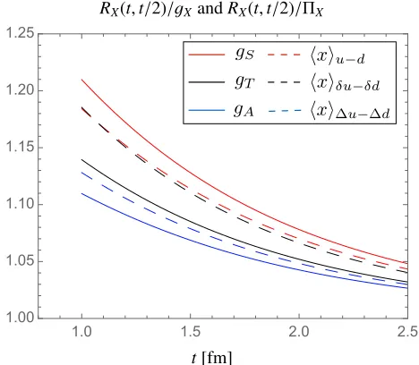
Qualitatively the same results are found for the tensor and scalar charges and the three moments. Fig.5shows the plateau estimates normalized by either the charge or the moment. As for the axial charge we only find a small dependence onM⇡L in all cases, so fig.5shows the M⇡L = 4 results only. In all cases we find the low-momentumN⇡states start to dominate fort&2 fm, thus the results displayed in fig.5are expected to be reliable only fort&2 fm.
RA(t,t/2)/gA
1.0 1.5 2.0 2.5
1.00 1.02 1.04 1.06 1.08 1.10 1.12 1.14 1.16
t[fm]
Figure 4.The plateau estimateRA(t,t/2) normalized bygAas a function of the source-sink separationt. Results
are shown forM⇡L = 4 (solid lines), M⇡L = 5 (dotted lines) andM⇡L = 6 (dashed lines). Di↵erent colors
distinguish between three di↵erent upper energy bounds for theN⇡states taken into account (see main text).
Fig.4 also shows that theN⇡contribution leads to an overestimation of the axial charge by the plateau estimate. Before reading o↵ a number from the plot recall that ChPT is an expansion in
small pion momenta. We may expect reasonably reliable ChPT results for the low-momentumN⇡ states, depicted by the black lines in the plot. The chiral expansion of the high-momentumN⇡states, included in the blue and red curves, is expected to work less well if it works at all.
This restriction implies that the source-sink separationtneeds to be large enough for the contri-bution of the high-momentum states to be sufficiently suppressed such that the low-momentum states
provide the dominate part of the totalN⇡contribution. According to fig.4this seems satisfied for
t⇡2.5 fm, but certainly not fort⇡1.5 fm where the low-momentum states contribute less than half of the contribution given by the red curves. It is at aboutt ⇡2 fm that the black lines start to cap-ture the dominantN⇡contribution, thus we may conclude that source-sink separations of about 2 fm and larger are required for ChPT to make reliable estimates. How large the higher order corrections at these source-sink separations are is difficult to predict. Naive error estimates suggest a 30-50%
uncertainty fort&2 fm. A more solid error estimate requires the calculation at NLO.
Qualitatively the same results are found for the tensor and scalar charges and the three moments. Fig.5shows the plateau estimates normalized by either the charge or the moment. As for the axial charge we only find a small dependence on M⇡Lin all cases, so fig.5shows the M⇡L = 4 results only. In all cases we find the low-momentumN⇡states start to dominate fort&2 fm, thus the results displayed in fig.5are expected to be reliable only fort&2 fm.
According to fig.5theN⇡-state contribution leads to an overestimation for all three charges and the three moments by their plateau estimates. The largest overestimation is found for the scalar charge, which is about twice as large as for the axial charge. TheN⇡contribution to the average momentum
RX(t,t/2)/gXandRX(t,t/2)/⇧X
Results: Midpoint estimate for all
charges and moments
x
u d
x
u d
x
u d
gS
gA
g
T1.0 1.5 2.0 2.5
1.00 1.05 1.10 1.15 1.20 1.25
t[fm]
Figure 5. The plateau estimatesRX(t,t/2) normalized by the asymptotic values for all charges and moments.
Results are shown forM⇡L =4 withN⇡states included with energies up to 1.6 GeV. The result for the axial
charge (blue solid line) is the same as the blue solid line in fig.4.
fraction is close to the one for the scalar charge. In summary we find an overestimation of about 5-10% for the charges and moments att⇡2 fm, and it slowly decreases to 3-6% att⇡2.5 fm.
We stress once again that these numbers are results at LO, i.e. at O(p). The higher order corrections are hard to quantify without having done the calculation at NLO. However, naive arguments can be made for the O(p2) corrections and suggest error estimates up to about 50%.
5 Comparison with lattice data
Most of the existing lattice results for the charges and moments have been obtained for pion masses larger than the physical value. There exist many reviews summarizing these results, for example Refs. [43–46]. Moreover, Sara Collins presented a review talk at Lattice 2016 in Southampton [47], and I refer to it for details concerning the present status of the lattice calculations.
Some collaborations have carried out lattice calculations with the pion mass at or near the physical value [48–53]. The main obstacle for directly applying the ChPT results to these lattice calculations are the rather small sink separations in these simulations. In most cases the maximal source-sink separation used to extract the charges and moments with the plateau method is below 1.5 fm. As discussed in the previous section, ChPT is not expected to provide solid results unless the source-sink separations are about 2 fm or even larger. Still, it is useful to compare the existing lattice results with our ChPT predictions, since the latter need to be reproduced eventually.
In the following we restrict ourselves to data obtained with the plateau method with pion masses not larger than 165 MeV. Lattice results obtained with the summation method [52], two-state fits [50] or the method based on the Feynman-Hellman theorem [9,54] cannot be used in our comparison.
gA,plat(t)/gA,exp
1.0 1.5 2.0 2.5
0.85 0.90 0.95 1.00 1.05 1.10
t[fm]
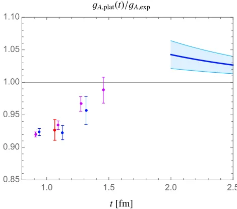
Figure 6.Lattice plateau estimates for the axial charge normalized by the experimental value. Lattice data from ETMC (blue), NME (magenta) and RQCD (red). The ChPT result of fig.5is also shown fort≥2 fm by the blue solid line together with a 50% error band as a naive estimate for higher order corrections.
Figure6shows the renormalized plateau estimates obtained by ETMC [49,55], NME [56,57] and RQCD [48], divided by the experimental valuegA,exp[6].8 The ETMC results (blue symbols) were obtained withNf =2 twisted mass fermions withM⇡ ⇡130 MeV,M⇡L⇡3 anda⇡0.093. The NME results (magenta symbols) were generated withNf =2+1 Wilson-clover fermions withM⇡ ⇡165 MeV,M⇡L ⇡ 3.7 anda ⇡0.09. The remaining data point (red symbol) from RQCD was obtained withNf =2 improved Wilson fermions withM⇡ ⇡150 MeV,M⇡L ⇡3.5 anda ⇡0.071 fm. More details about the simulation setup are given in the original papers.
The plateau estimates shown in fig.6were obtained for source-sink separations between 0.9 and 1.5 fm. They are all below the experimental value although the NME result att⇡1.5 fm agrees with gA,expwithin the statistical error.
The ChPT prediction for the overestimation due to theN⇡states is also shown fort ≥2 fm. A naive guess for the higher order corrections is also included in form of a 50% error band. Apparently, the lattice data is not in conflict with the ChPT result. It seems very plausible that the lattice data will connect smoothly to the ChPT prediction whentis increased. Whether this indeed happens needs to be checked. This requires lattice calculations ofgAattlarger than 1.5 fm with a statistical error of a few percent.9
If indeed realized, such a scenario can be quite misleading in practice. Since the plateau estimate approaches the experimental value at sometwell before the asymptotic region is reached, one might be tempted to stop simulating at larger source-sink separations. In that case one reproduces the correct experimental valuegA,exp, but for the wrong reason. The excited-state contributions are not small be-8The ETMC results shown in fig.6are based on larger statistics compared to the ones given in Ref. [49]. They have smaller error bars but are still preliminary [55]. I thank C. Alexandrou and C. Kallidonis for sharing these results. I also thank R. Gupta, Y.-C. Jang and B. Yoon for sending me numerical results published in Ref. [56].
gA,plat(t)/gA,exp
1.0 1.5 2.0 2.5
0.85 0.90 0.95 1.00 1.05 1.10
t[fm]
Figure 6.Lattice plateau estimates for the axial charge normalized by the experimental value. Lattice data from ETMC (blue), NME (magenta) and RQCD (red). The ChPT result of fig.5is also shown fort≥2 fm by the blue solid line together with a 50% error band as a naive estimate for higher order corrections.
Figure6shows the renormalized plateau estimates obtained by ETMC [49,55], NME [56,57] and RQCD [48], divided by the experimental valuegA,exp[6].8 The ETMC results (blue symbols) were obtained withNf =2 twisted mass fermions withM⇡ ⇡130 MeV,M⇡L⇡3 anda⇡0.093. The NME results (magenta symbols) were generated withNf =2+1 Wilson-clover fermions withM⇡ ⇡165 MeV,M⇡L ⇡ 3.7 anda ⇡ 0.09. The remaining data point (red symbol) from RQCD was obtained withNf =2 improved Wilson fermions with M⇡ ⇡150 MeV,M⇡L ⇡3.5 anda ⇡0.071 fm. More details about the simulation setup are given in the original papers.
The plateau estimates shown in fig.6were obtained for source-sink separations between 0.9 and 1.5 fm. They are all below the experimental value although the NME result att⇡1.5 fm agrees with gA,expwithin the statistical error.
The ChPT prediction for the overestimation due to theN⇡states is also shown fort ≥2 fm. A naive guess for the higher order corrections is also included in form of a 50% error band. Apparently, the lattice data is not in conflict with the ChPT result. It seems very plausible that the lattice data will connect smoothly to the ChPT prediction whentis increased. Whether this indeed happens needs to be checked. This requires lattice calculations ofgAattlarger than 1.5 fm with a statistical error of a few percent.9
If indeed realized, such a scenario can be quite misleading in practice. Since the plateau estimate approaches the experimental value at sometwell before the asymptotic region is reached, one might be tempted to stop simulating at larger source-sink separations. In that case one reproduces the correct experimental valuegA,exp, but for the wrong reason. The excited-state contributions are not small be-8The ETMC results shown in fig.6are based on larger statistics compared to the ones given in Ref. [49]. They have smaller error bars but are still preliminary [55]. I thank C. Alexandrou and C. Kallidonis for sharing these results. I also thank R. Gupta, Y.-C. Jang and B. Yoon for sending me numerical results published in Ref. [56].
9In addition one should also check that the underestimation of the axial charge at small source-sink separations persists in the continuum limit.
causetis sufficiently large to be in the asymptotic regime. Instead, various excited-state contributions
are still sizeable but accidentally cancel each other.
A concrete model for such a scenario was suggested by M. Hansen and H. Meyer in Ref. [58]. Based on plausible assumptions concerning the higher order corrections to the LO ChPT results, the high-momentumN⇡states with energies larger than about 1.5 MN contributenegativelyto the plateau estimate. Summing up the totalN⇡contamination the positive contribution from the low-momentum states is overcompensated by the contribution from the high-low-momentum states, leading to an underestimation of the axial charge for source-sink separations below about 1.5 fm, in agreement with lattice results.
Whether the high-momentumN⇡states are indeed responsible for the compensation of the low-momentum ones needs to be corroborated. Other excited states (e.g.N⇡⇡and∆⇡states) are expected to play a non-negligible role too for source-sink separations below 2 fm. In any case, the model in Ref. [58] supports the expectation that source-sink separationst&2 fm are needed for the LO ChPT results to be applicable.
Fig. 7 shows the plateau estimates of ETMC [49,55] and RQCD [53] for the average quark momentum fractionhxiu−dand the helicity momenthxi∆u−∆d, normalized by their phenomenological values given in [8,42]. For both observables the plateau estimates overestimate the phenomenological value. The absolute discrepancy is significantly larger than for the axial charge (note the di↵erent
scales in fig.7). The statistical errors are rather large, but the plots suggest that the plateau estimates decrease as the source-sink separation increases. Compared with the results for the axial charge it is here much simpler to imagine a simple monotonic decrease until contact with ChPT can be made at source sink-separations between 2 and 2.5 fm.
In case of the scalar and tensor charges as well as the transversity moment we do not have ex-perimental values at our disposal. Thus, comparisons between the lattice plateau estimates and the ChPT predictions cannot be done. However, there is no reason to believe that the asymptotic region is reached at significantly smaller source-sink separations for these observables. In fact, the absence of experimental results elevates the role ChPT can play as a guide for the systematic uncertainties due theN⇡states, provided one is in the asymptotic regime where ChPT can be applied.
The main conclusion we can draw from our comparison is that present lattice data at source-sink separationst.1.5 fm is still far away from the asymptotic regime where the lowest lyingN⇡states are responsible for the dominant excited-state contribution in the plateau estimates. Lattice data at significantly larger source-sink separations (and with sufficiently small statistical errors) are needed
to make contact with the asymptotic region where ChPT can be applied.
6 Miscellaneous comments
An alternative way to compute the charges and pdf moments is provided by the summation method [59, 60]. It starts from the ratio RX(t,t0) and computes the sum over all operator insertion times between source and sink. In case of the axial charge the result of the sum is of the form
t X
t0=0
RA(t,t0)=t[gA+O(e−∆Ent)]+. . . . (10)
The slope [. . .] is called the summation estimate of the axial charge. For finitetit di↵ers by
exponen-tially suppressed excited state contributions fromgA.
Using the ChPT results for the ratios in eq. (10) theN⇡-state contribution to the summation es-timate is easily computed. However, the sum on the left hand side involves the 3pt function at short
hxiu−d,plat(t)/hxiu−d,phen
1.0 1.5 2.0 2.5
1.0 1.1 1.2 1.3 1.4 1.5
t[fm]
hxi∆u−∆d,plat(t)/hxi∆u−∆d,phen
1.0 1.5 2.0 2.5
1.0 1.1 1.2 1.3 1.4 1.5
t[fm]
hxiu−d,plat(t)/hxiu−d,phen
1.0 1.5 2.0 2.5
1.0 1.1 1.2 1.3 1.4 1.5
t[fm]
hxi∆u−∆d,plat(t)/hxi∆u−∆d,phen
1.0 1.5 2.0 2.5
1.0 1.1 1.2 1.3 1.4 1.5
t[fm]
Figure 7. Lattice plateau estimates for the average momentum fraction (upper panel) and the helicity moment (lower panel) normalized by their phenomenological values. Lattice data from ETMC (blue) and RQCD (red). The ChPT result of fig.5is also shown fort≥2 fm together with a 50% error band as a naive estimate for higher order corrections.
Me↵(t)/MN
0.6 0.8 1.0 1.2 1.4 1.6 1.8 2.0
1.00 1.01 1.02 1.03 1.04
t[fm]
Figure 8.The ratioMN,e↵(t)/MNas a function of the source sink separationt. Results are shown forM⇡L=4
(solid lines),M⇡L =5 (dotted lines) andM⇡L =6 (dashed lines). Di↵erent colors distinguish between three
di↵erent upper energy bounds for theN⇡states taken into account (see main text).
distances whent0approaches either source or sink. In these cases the ChPT results do not properly capture the full 3pt function and the ratio.
A possible remedy for this limitation would be to keep all time separations large by summing over a central subinterval only. This, however, requires even larger source-sink separations than those needed for the plateau method. Based on our results we would expect to need a minimal separation of about 1 fm fort−t0andt0. In addition we need a non-zero time interval to sum over. Both requirements imply minimal source-sink separations of about 2.5 fm if not larger. Note that this is not a requirement for the summation method per se, but for ChPT to have something to say about it.
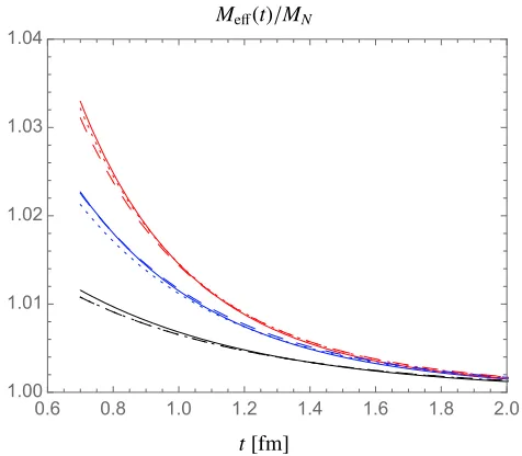
For the computation of the various ratios we had to compute the 2pt function. It is interesting to also look at theN⇡contribution to the e↵ective nucleon mass, c.f. eg. (3). Fig.8shows the ratio
MN,e↵(t)/MN as a function of the source-sink separationt. Without the excited state contribution this ratio would be equal to 1, any deviation from this value stems from theN⇡contribution. As in figure
4, results are shown for the three di↵erent lattice sizes (solid, dashed and dotted lines) and the three
di↵erent energiesEN⇡,nmax(black, blue and red lines) considered before.
Qualitatively figs.4and8look very similar. Only a very small FV dependence is visible, provided the number of states are adjusted according to the energy interval for theN⇡states taken into account for theN⇡contribution. The largertthe more dominates the contribution of the low-momentumN⇡ states (black curves). The actual timetwhere this happens, however, is much smaller compared to the result for the axial charge. Even more importantly, theN⇡state contamination in the e↵ective
mass is significantly smaller. Even allowing for an error as big as 100% for theN⇡contribution the overestimation of the nucleon mass is smaller than 2% at source-sink separations of about 1.2 fm and larger. This contamination can be ignored unless the lattice data have statistical errors at the sub-percent level.
Note that the significantly larger excited-state contamination in the charges and moments stems from the contributions associated with the time separationst −t0 andt0. For this reason the N⇡ contribution at a given timetin fig.8should be compared the one at 2tin fig.4. In that case theN⇡ contribution in both observables is roughly of the same size.10
The conclusions we have drawn are based on the LO results for theN⇡-state contribution. This contribution dominates for large time separations in physical point simulations. A calculation of the NLO corrections is certainly desirable, mainly to obtain firmer error estimates for the LO results. In addition, it needs to be checked that contributions of other excited states are small and do not change qualitatively the results we have found. Other multi-hadron-state contributions have their origin in three-particleN⇡⇡states and two-particle∆⇡states. ChPT calculations of these contributions are essentially analogous to the calculation of the N⇡ contribution and in principle straightforward to perform.
7 Conclusions
Physical point simulations eliminate the systematic uncertainties associated with a chiral extrapola-tion. Excited-state e↵ects due to multi-hadron-states involving one or more pions, on the other hand,
become more pronounced for pion masses as light as in nature. Using Baryon ChPT we have com-puted the two-particleN⇡state contamination in the plateau estimates of various nucleon charges and pdf moments. This particular excited-state contamination leads to an overestimation at the 5-10% level for source-sink separations of about 2 fm. This is uncomfortably large and cannot be not ignored if results with percent precision are the goal of lattice calculations.
Even more troublesome is that lattice calculations of the charges and moments with source-sink separations of 2 fm and larger are out of reach with present simulation techniques. So far most lattice results have been obtained with source-sink separations of 1.5 fm and smaller. At time separations that small one expects excited states other thanN⇡states to contribute a sizeable excited-state con-tamination too.
In case of the axial charge the lattice data together with the ChPT result strongly suggests a non-monotonict dependence of the plateau estimate. The lattice data underestimate the experimental value fort.1.5 fm while ChPT predicts an overestimation for larger time separations. This peculiar behavior, neither seen for the average quark momentum fraction nor the helicity moment, can be attributed to other excited states that contribute a negative contamination to the plateau estimate. In this case we expect a cancellation of the various excited-state contributions for some source-sink separation and an accidental agreement between the lattice result and the experimental value for the axial charge. Given the benchmark character ofgA it thus seems vital to carefully check the excited-state contamination in this quantity with lattice simulations at source-sink separations larger than 1.5 fm.
The main conclusion we can draw from our ChPT calculation is that physical point simulations require significantly larger source-sink separations than those with heavier pion masses. Simulations with larger time separations require new simulation techniques to overcome the notorious signal-to-noise problem. Some ideas in that respect have been recently proposed [61–63] and presented at this conference [64,65], but remain to be tested in actual lattice calculations of the nucleon correlation functions considered here.
Alternatively one may resort to the variational method [66,67] to get a handle on the nucleon ma-trix elements at smaller time separations. The variational method can be used provided interpolating
10The factors∆En/MNinMe
↵/MN, c.f. eq. (3), causes an additional suppression of the excited-state contribution in the
Note that the significantly larger excited-state contamination in the charges and moments stems from the contributions associated with the time separationst −t0 andt0. For this reason the N⇡ contribution at a given timetin fig.8should be compared the one at 2tin fig.4. In that case theN⇡ contribution in both observables is roughly of the same size.10
The conclusions we have drawn are based on the LO results for theN⇡-state contribution. This contribution dominates for large time separations in physical point simulations. A calculation of the NLO corrections is certainly desirable, mainly to obtain firmer error estimates for the LO results. In addition, it needs to be checked that contributions of other excited states are small and do not change qualitatively the results we have found. Other multi-hadron-state contributions have their origin in three-particleN⇡⇡states and two-particle∆⇡states. ChPT calculations of these contributions are essentially analogous to the calculation of the N⇡contribution and in principle straightforward to perform.
7 Conclusions
Physical point simulations eliminate the systematic uncertainties associated with a chiral extrapola-tion. Excited-state e↵ects due to multi-hadron-states involving one or more pions, on the other hand,
become more pronounced for pion masses as light as in nature. Using Baryon ChPT we have com-puted the two-particleN⇡state contamination in the plateau estimates of various nucleon charges and pdf moments. This particular excited-state contamination leads to an overestimation at the 5-10% level for source-sink separations of about 2 fm. This is uncomfortably large and cannot be not ignored if results with percent precision are the goal of lattice calculations.
Even more troublesome is that lattice calculations of the charges and moments with source-sink separations of 2 fm and larger are out of reach with present simulation techniques. So far most lattice results have been obtained with source-sink separations of 1.5 fm and smaller. At time separations that small one expects excited states other thanN⇡states to contribute a sizeable excited-state con-tamination too.
In case of the axial charge the lattice data together with the ChPT result strongly suggests a non-monotonict dependence of the plateau estimate. The lattice data underestimate the experimental value fort.1.5 fm while ChPT predicts an overestimation for larger time separations. This peculiar behavior, neither seen for the average quark momentum fraction nor the helicity moment, can be attributed to other excited states that contribute a negative contamination to the plateau estimate. In this case we expect a cancellation of the various excited-state contributions for some source-sink separation and an accidental agreement between the lattice result and the experimental value for the axial charge. Given the benchmark character ofgAit thus seems vital to carefully check the excited-state contamination in this quantity with lattice simulations at source-sink separations larger than 1.5 fm.
The main conclusion we can draw from our ChPT calculation is that physical point simulations require significantly larger source-sink separations than those with heavier pion masses. Simulations with larger time separations require new simulation techniques to overcome the notorious signal-to-noise problem. Some ideas in that respect have been recently proposed [61–63] and presented at this conference [64,65], but remain to be tested in actual lattice calculations of the nucleon correlation functions considered here.
Alternatively one may resort to the variational method [66,67] to get a handle on the nucleon ma-trix elements at smaller time separations. The variational method can be used provided interpolating
10The factors∆En/MNinMe
↵/MN, c.f. eq. (3), causes an additional suppression of the excited-state contribution in the
e↵ective mass.
fields for theN⇡states are taken into account [68–71]. In this approach too the numerical cost grows significantly since the number of Wick contractions involved in computing the correlation functions grows rapidly once interpolating fields for multi-particle states are used [70].
Acknowledgments
Communication with C. Alexandrou, R. Gupta, Y.-C. Jang, M. Kallidonis and R. Sommer is gratefully acknowledged. This work was supported by the Japan Society for the Promotion of Science (JSPS) with an Invitation Fellowship for Research in Japan (ID No. L16520), and by the German Research Foundation (DFG), Grant ID BA 3494/2-1.
References
[1] G. Parisi, Phys. Rept.103, 203 (1984)
[2] G.P. Lepage,The Analysis of Algorithms for Lattice Field Theory, inBoulder ASI 1989:97-120
(1989), pp. 97–120,http://alice.cern.ch/format/showfull?sysnb=0117836 [3] M. Lüscher, Nucl. Phys.B364, 237 (1991)
[4] K.I. Ishikawa, N. Ishizuka, Y. Kuramashi, Y. Nakamura, Y. Namekawa, Y. Taniguchi, N. Ukita, T. Yamazaki, T. Yoshie (PACS), PoSLATTICE2015, 075 (2016),1511.09222
[5] Y. Kuramashi, A large scale simulation of 2+1 flavor lattice QCD, talk at this conference,
https://makondo.ugr.es/event/0/session/94/contribution/175 [6] C. Patrignani et al. (Particle Data Group), Chin. Phys.C40, 100001 (2016)
[7] T. Bhattacharya, V. Cirigliano, S.D. Cohen, A. Filipuzzi, M. Gonzalez-Alonso, M.L. Graesser, R. Gupta, H.W. Lin, Phys. Rev.D85, 054512 (2012),1110.6448
[8] S. Alekhin, J. Blümlein, S. Moch, Phys. Rev.D86, 054009 (2012),1202.2281
[9] C. Bouchard, C.C. Chang, T. Kurth, K. Orginos, A. Walker-Loud, Phys. Rev. D96, 014504 (2017),1612.06963
[10] O. Bär, Phys. Rev.D92, 074504 (2015),1503.03649 [11] O. Bär, Phys. Rev.D94, 054505 (2016),1606.09385 [12] O. Bär, Phys. Rev.D95, 034506 (2017),1612.08336
[13] O. Bär, Int. J. Mod. Phys.A32, 1730011 (2017),1705.02806 [14] B.C. Tiburzi, Phys. Rev.D80, 014002 (2009),0901.0657
[15] O. Bär, M. Golterman, Phys. Rev.D87, 014505 (2013),1209.2258 [16] M. Lüscher, PoSLATTICE2013, 016 (2014),1308.5598
[17] O. Bär, M. Golterman, Phys.Rev.D89, 034505 (2014),1312.4999 [18] S. Weinberg, PhysicaA96, 327 (1979)
[19] J. Gasser, H. Leutwyler, Ann. Phys.158, 142 (1984) [20] J. Gasser, H. Leutwyler, Nucl. Phys.B250, 465 (1985)
[21] G. Colangelo, G. Isidori,An Introduction to ChPT, inNuclear, subnuclear and astroparticle physics. Proceedings, 5th LNF Spring School, Frascati, Italy, May 15-20, 2000(2000), pp. 333– 376,hep-ph/0101264,http://weblib.cern.ch/abstract?CERN-TH-2001-019
[22] J. Gasser, Lect. Notes Phys.629, 1 (2004),hep-ph/0312367
[23] B. Kubis,An Introduction to chiral perturbation theory, in Workshop on Physics and Astro-physics of Hadrons and Hadronic Matter Shantiniketan, India, November 6-10, 2006 (2007), hep-ph/0703274
[24] S. Scherer, Prog. Part. Nucl. Phys.64, 1 (2010),0908.3425
[25] M. Golterman,Applications of chiral perturbation theory to lattice QCD, inModern perspec-tives in lattice QCD: Quantum field theory and high performance computing. Proceedings, In-ternational School, 93rd Session, Les Houches, France, August 3-28, 2009(2009), pp. 423–515, 0912.4042,
[26] S. Scherer, M.R. Schindler, Lect.Notes Phys.830, pp.1 (2012) [27] G. Ecker, Nucl. Phys. Proc. Suppl.245, 1 (2013),1310.2084 [28] V. Bernard, Prog. Part. Nucl. Phys.60, 82 (2008),0706.0312 [29] J. Gasser, M. Sainio, A. Svarc, Nucl.Phys.B307, 779 (1988)
[30] T. Becher, H. Leutwyler, Eur.Phys.J.C9, 643 (1999),hep-ph/9901384
[31] N. Fettes, U.G. Meissner, M. Mojzis, S. Steininger, Annals Phys. 283, 273 (2000), hep-ph/0001308
[32] M. Dorati, T.A. Gail, T.R. Hemmert, Nucl. Phys.A798, 96 (2008),nucl-th/0703073 [33] P. Wein, P.C. Bruns, A. Schäfer, Phys. Rev.D89, 116002 (2014),1402.4979
[34] K. Nagata, A. Hosaka, V. Dmitrasinovic, Eur.Phys.J.C57, 557 (2008) [35] B. Io↵e, Nucl.Phys.B188, 317 (1981)
[36] D. Espriu, P. Pascual, R. Tarrach, Nucl.Phys.B214, 285 (1983)
[37] P. Wein, P.C. Bruns, T.R. Hemmert, A. Schäfer, Eur.Phys.J.A47, 149 (2011),1106.3440 [38] S. Güsken, U. Low, K. Mutter, R. Sommer, A. Patel et al., Phys.Lett.B227, 266 (1989) [39] S. Güsken, Nucl.Phys.Proc.Suppl.17, 361 (1990)
[40] C. Alexandrou, F. Jegerlehner, S. Güsken, K. Schilling, R. Sommer, Phys.Lett.B256, 60 (1991) [41] M. Lüscher, JHEP1304, 123 (2013),1302.5246
[42] J. Blümlein, H. Böttcher, Nucl. Phys.B841, 205 (2010),1005.3113 [43] S. Syritsyn, PoSLATTICE2013, 009 (2014),1403.4686
[44] J. Green, AIP Conf. Proc.1701, 040007 (2016),1412.4637 [45] M. Constantinou, PoSCD15, 009 (2015),1511.00214
[46] C. Alexandrou, EPJ Web Conf.137, 01004 (2017),1612.04644
[47] S. Collins,Hadron Structure, plenary talk given at34th International Symposium on Lattice Field Theory (Lattice2016), Southampton, UK, 26th July 2016,
https://conference.ippp.dur.ac.uk/event/470/session/1/contribution/118 [48] G.S. Bali, S. Collins, B. Glässle, M. Göckeler, J. Najjar, R.H. Rödl, A. Schäfer, R.W. Schiel,
W. Söldner, A. Sternbeck, Phys. Rev.D91, 054501 (2015),1412.7336
[49] A. Abdel-Rehim et al., Phys. Rev. D92, 114513 (2015), [Erratum: Phys. Rev.D93,no.3,039904(2016)],1507.04936
[50] T. Bhattacharya, V. Cirigliano, S. Cohen, R. Gupta, H.W. Lin, B. Yoon (2016), arXiv:1606.07049 [hep-lat]
[51] G. von Hippel, T.D. Rae, E. Shintani, H. Wittig, Nucl. Phys.B914, 138 (2017),1605.00564 [52] J.R. Green, M. Engelhardt, S. Krieg, J.W. Negele, A.V. Pochinsky, S.N. Syritsyn, Phys. Lett.
B734, 290 (2014),1209.1687
[53] G.S. Bali, S. Collins, B. Gläßle, M. Göckeler, J. Najjar, R.H. Rödl, A. Schäfer, R.W. Schiel, A. Sternbeck, W. Söldner, Phys. Rev.D90, 074510 (2014),1408.6850
[54] E. Berkowitz et al. (2017),1704.01114
[55] C. Alexandrou and C. Kallidonis, private communication, June 2017 [56] B. Yoon et al., Phys. Rev.D95, 074508 (2017),1611.07452