Focussed information criteria and model averaging for Cox's hazard regression model.

FOCUSSED INFORMATION CRITERIA AND MODEL AVERAGING FOR COX'S HAZARD REGRESSION MODEL

Focussed information criteria and model averaging

for Cox's hazard regression model

Nils Lid Hjort and Gerda Claeskens

University of Oslo and Katholieke U niversiteit Leuven

November 2004

ABSTRACT. This article is concerned with variable selection methods for the pro-portional hazards regression model. Including too many covariates causes extra variability and inflated confidence intervals for regression parameters, so regimes for discarding the less informative ones are needed. Our framework has p covari-ates designated as 'protected' while variables from a further set of q covariates are examined for possible in- or exclusion. In addition to deriving results for the AIC method, defined via the partial likelihood, we develop a focussed information cri-terion that for given interest parameter finds the best subset of covariates. Thus the FIC might find that the best model for predicting median survival time might be different from the best model for estimating survival probabilities, and the best overall model for analysing survival for men might not be the same as the best overall model for analysing survival for women. We also develop methodology for model averaging, where the final estimate of a quantity is a weighted average of estimates computed for a range of submodels. Our methods are illustrated in simulations and for a survival study of Danish skin cancer patients.

KEY WORDS: Akaike's information criterion, covariate selection, Cox regression, focussed information criteria, median survival time, model averaging

1. Introduction and summary

Suppose survival data of the form (ti' Oi, Xi, Zi) are recorded for n individuals, where ti is

life-time, possibly censored, Oi is an indicator for non-censoring, Xi contains say p covariates that are deemed necessary in the regression model, while Zi has say q further covariates potentially worthy of inclusion. The most popular model for such data is the Cox model of proportional hazards, where the hazard rate for individual i is expressed as

hi(u) = ho(u) exp(x;,6

+

z;,) for i = 1, ... , n. (1.1 ) Here h

o( u)

is assumed to be continuous and positive over the range of life-times of interest, but is otherwise not specified. This makes the model partly parametric and partly nonpara-metric. Inference about

(,6,,)

typically proceeds using the well-known partial likelihood

Ln

(,6,,),

properly defined in Section 2.

This article is concerned with developing methods for selecting the in some sense best covariates Zi,j among the q. The argument against simply including all of them is that this may cause too much estimation variability, leading to inflated confidence intervals and less powerful tests. On the other hand including too few covariates could mean serious modelling bias and missing important explanatory features in the analysis. Thus selecting 'the best' set is a statistical balancing act between bias and variance.

1.1. The Danish malignant melanoma study. For an illustration we study the skin cancer survival analysis data set that is described and analysed extensively in Andersen, Borgan, Gill and Keiding (1993) and elsewhere. In this Danish study, 205 patients with malignant melanoma had radical removal surgery and were followed after operation over the time period 1962-1977. Several covariate variables are of potential interest for studying survival chances, including

Xl, indicator for sex of the patient (woman

=

1, man

=

2);

Zl, thickness of the tumour, more precisely Zl = (z~

-

292)/100 where z~ is the real thickness, in 1/100 mm, with the average value 292 subtracted out;

Z2, infection infiltration level, a measure of resistance against the tumour, from high

resistance 1 down to low resistance 4);

Z3, presence indicator of so-called epithelioid cells (present

=

1, non-present

=

2); Z4, ulceration presence (present

=

1, non-present

=

2);

Z5, invasion depth (at levels 1, 2, 3); and

Z6, age of the patient at the operation (in years).

Patients dead of other causes or still alive in 1977 are treated as censored observations. Among the findings in Andersen et al. (1993) were that men tend to have higher hazard than women. That is why we designate Xl as 'protected' here, and look for 'the best'

covariates to keep among Zl, . . . , Z6. Data rows for the first five and the last five of the 205

are as follows (we have sorted the 205 rows by increasing life-times). Here Ci is 1 if dead

from the illness, 2 if censored, and 4 if dead from other reasons, so that

Oi

=

I

{ci = I}.

ti

Ci Xl Zl Z2 Z3 Z4 Z5 Z6 1 10 4 2 3.84 3 2 1 2 76 2 30 4 2 -2.27 1 1 2 1 56 3 35 2 2 -1.58 3 1 2 2 41 4 99 4 1 -0.02 3 1 2 1 71 5 185 1 2 9.16 3 2 1 3 52 201 4492 2 2 4.14 4 2 1 3 29 202 4668 2 1 3.20 3 2 2 3 40 203 4688 2 1 -2.44 2 2 2 1 42 204 4926 2 1 -0.66 2 1 2 1 50 205 5565 2 1 -0.02 3 1 2 2 41

TABLE 1.1. The first five and the last five rows from the Danish malignant melanoma survival data set, with life-times

ti

(in days), censoring indicator Ci,

and covariates Xl, Zl, . . . ,Z6 as described above.

1.2. Some selection methods. There are rather few well-developed variable selection methods for the Cox model. Methods involving pre-testing of coefficients and variants of backward and forward regression can be put forward, in partial analogy with linear or generalised linear regression theory; we know of no serious study of the performance of such methods in the Cox model context, however. The general model averaging theory

we develop in Section 8 below will actually accurately describe the performance of such methods. Fan and Li (2002) propose a penalised version of the log-partial likelihood, with a penalty called the smoothly clipped absolute deviation. This penalty depends on two unknown parameters where the first is fixed at a pre-determined value while the second is chosen via an approximation to generalised cross-validation. Tibshirani (1997) uses the lasso method for variable selection in the Cox model; this and similar L1 based methods refined later in Efron, Hastie, Johnstone and Tibshirani (2004) are of particular value when the number q of non-protected covariates is large. Bunea and McKeague (2004) also introduce a penalised partial likelihood, where now the penalty depends on both the number of parameters in the parametric part of the model and on the number of components in the sieve construction to estimate the unknown baseline hazard function.

More traditional model selection methods such as AIC and BIC are not automatically defined for Cox models, since there is no workable full likelihood for data. One may however choose to use the partial likelihoods, say

Ln,s

for the model that only uses covariates Zi,j

for j E S, which leads to

AICn,s

= 2 log

Ln,s(!3s,-;;;s) -

2(p+

lSI),

BIen,s

= 2 log

Ln,sC!3s, -;;;s) -

(p

+

lSI)

log n,

(1.2)

in terms of the Cox estimators

(!3s,-;;;s)

inside the

S

submodel. Here

lSI

denotes the number of elements in S, and the model with the highest score is selected. These model selection schemes are easily implemented using software for handling the Cox regression model. Volinsky and Raftery (2000) investigate some aspects of the BIC scheme, including discussion of other penalty factors, along with versions of Bayesian model averaging strate-gies for the Cox model. Less theory has however been developed for the AI C and BI C methods valid for the Cox model than for fully parametric regression models. It should be noted that these criteria work only with the parametric part of the (1.1) model, thus ignoring the nonparametric part. It is therefore not clear whether model selectors using (1.2) are relevant when it comes to consequences for questions that relate to all of the (1.1) model, like survival probabilities and median survival time. For the melanoma data set, at any rate, the AIC method selects variables 2, 3, 4, 5, 6 among the Zi,jS while the BIC

regime chooses variables 4, 5.

1.3. Focussed information criteria and model averaging. Different selection method find different 'best subsets', as dramatically witnessed for the Danish melanoma data set with the AIC and the Ble. What all the methods mentioned above have in common is however that they advocate one and only one final model, regardless of its intended use, whether this involves predicting median survival time or estimating survival chances for patients with unusual characteristics and so on. We shall develop a certain 'focussed information criterion', the FIC, that for each parameter of interest finds the best submodel for that purpose. Specifically, for a given focus parameter {-L({3,

r,

Ho),

where

Ho

is the

cumulative baseline hazard rate, we are able to estimate the mean squared error for each of the many candidate estimators, say

lis

for the model indexed by subset

S.

The FIC strategy is to select the model with lowest possible mean squared error estimate.

We do not view this as a paradox, even if it means leaving behind the traditionally strong and conceptually sirening paradigm of finding one adequate model to explain all aspects and facets of the data. Thus for the Danish skin cancer data we shall see in Section 9 that when it comes to estimating a certain relative risk parameter, then the FIC selects the narrow model as the best one, with only Xl and none of the ZjS; while for estimating

a certain survival probability, FIC chooses to include Z5.

When a model selection scheme like the AIC or FIC is followed to produce an estimator it is important to realise that the real variance involved is larger than if the selected model had been given in advance. Studying statistical properties of such post-selection estimators involves more work than simply understanding the limit distributions of the Cox estimators. In our article we reach precise large-sample results for a broad class of 'compromise estimators' that interpolate between all candidate models, with the post-selection estimators constituting special cases. The limit distributions involved are not normal, but rather non-linear mixtures of different normals.

The theory and results for our FIC and model average estimators parallel development and findings in our earlier articles Claeskens and Hjort (2003) and Hjort and Claeskens (2003a, 2003b), hereafter referred to as CH and HC (2003). These articles were concerned with likelihood methods for general parametric models, including various regression mod-els, but the results reached there do not capture and cannot be applied directly inside the Cox regression model. This is partly because of the censoring and of the semiparametric nature of model (1.1), rendering analysis of estimators that combine both H

o

and ((3, ,) estimators difficult. Thus a separate development for building a proper FIC along with proper model average methods for the Cox model has been necessary.

We learn in doing so that the CH and HC (2003) theory and methods carryover with reasonable ease to situations which involve only the regression parameters ((3, I); in other words, as long as questions are posed that can be answered in terms of ((3,

I),

one does not need significant extensions of the already available theory. This comment will be seen to apply also to results for the AIC strategy. Many questions of interest relate however to the full (1.1) model, including the hazard rate part, like the median survival time

HOI

(log

2j

exp(xt(3

+

zt,)), the survival probability exp{-exp(xt(3

+

zt,)Ho(t)},

likewise conditional survival probabilities given than one has survived up to a certain time point, etc. It is for such questions that the CH and HC (2003) theory needs harder work to be appropriately extended, as seen in the sections to follow.

1.4. The present article. Our article is organised as follows. Section 2 sets the basic framework, properly defining all subset estimators

lis

for a given focus parameter

large-sample approximations to modelling bias, variance, and distributions of estimators. In Sections 3 and 4 we develop theory for describing the behaviour of submodel-based estimators

/3s

and

1s

for the regression coefficients and

Ho,s

for the cumulative hazard. This is used in Section 5 to provide precise large-sample results for limit distributions and limiting risk for all submodel estimators. This is a harder task than proving limit theorems for the Cox estimators, in that these need to be studied also outside model conditions and since we need to care about simultaneous aspects of all the estimators involved.

In Section 6 we go through a list of particularly important parameters of interest, including survival probability curves for given strata of patients, median survival times, and relative risks. This is also where we describe how to estimate various quantities necessary for implementing the FIC methods. Section 7 gives the proper machinery for the FIC and its averaged versions. Then in Section 8 a 'master theorem' is provided that accurately describes the limit distribution for a large class of model average estimators. This in particular provides precise descriptions of the large-sample behaviour of all post-selection strategies, like the AIC and the FIC. Section 9 illustrates our methods in some settings with simulated data and goes on to analyse the Danish melanoma survival data set. Our article ends with a list of concluding remarks in Section 10, some of which might lead to further research work, and with Section 11, where we gather all proofs of lemmas from earlier sections.

2. A framework for covariate subset selection

Working inside the (1.1) model, with life-time data observed or partly observed over a time horizon [0,

T],

the log-partial likelihood can be written

log

Ln

C8,

1') =

tiT

[x~,8

+

zi'Y -

log{t

Yi( u)

exp(x~,8

+

zi'Y) } ]

dNi (

u),

(2.1)

i=l 0 i=l

where

Yi(u)

=

I{ti

2::

u}

and

dNi(u)

=

_I{ti

E

[u,u

+

du],oi

= I}. The maximum partial likelihood estimators, also referred to as the Cox estimators, are the

(/3,1)

values maximising (2.1). The theory to be developed in our article will partly utilise the large-sample theory associated with counting processes and martingales, as exposited e.g. in Andersen et al. (1993), where results are most comfortably reached if the upper time limit

T is finite, so we shall assume it to be so; somewhat more technical assumptions are needed

if one wishes to obtain results valid for T = 00.

For each subset S of

{I, ... ,q}

we may study the model indexed by

(,8,'Ys),

where 'Ys contains precisely those 'Yj coefficients where j E S, i.e. corresponding to including in the model only those Zi,j where j E S, excluding those with j

tt

S. There is a total

of 2q _{such submodels to consider. Sometimes several of these might be ruled out on a}

priori grounds, e.g. when there is a natural ordering in complexity, in which case only the

q

+

1 nested submodels of

{I, ... ,q}

are considered. For each submodel S there are

Cox estimators

(/3s,;;Ys),

and also an accompanying Aalen-Breslow type estimator of the cumulative baseline hazard function, namely

ii

(t)

=

it

L~l

dNii

u)

o,S n t t ~ ,

o Li=l

Yi(u)

exp(xi;Js

+

Zi,S'S)

(2.2)

where Zi,S means the components Zi,j of Zi for which j E

S.

For given estimand of interest, say ~ = ~(;J", H

o),

there is accordingly a list of potential estimators

(2.3) one for each submodel. The notation indicates that one uses the null value

,j

0 for

j tJ- S, i.e. for j E

se,

the complement set. The ~ in question may also depend on covariate positions

x

and

z,

as exemplified in Sections 6 and 9.

We shall study questions of covariate inclusion and exclusion inside a large-sample framework where, is small or moderate, and where the largest of the models, the one containing all p

+

q covariates, contains the truth. More specifically, the real hazard rate functions are taken to be

hi,true(u)

=

ho(u)

exp(x;;J

+

z;7]/vin)

for i = 1, ... , n, (2.4) for suitable (;J1, ... ,;Jp)t and (7]1, ... ,

7]q)t.

This turns out to be a fruitful framework for deriving accurate approximations to modelling bias and variances and hence mean squared errors for different estimators, essentially because variances and squared biases now become exchangeable currencies, both of order O(l/n). See also the general discussion surrounding these issues in CH and HC (2003).

3. Submodel estimators for hazard regression coefficients

This section develops theory for the large-sample behaviour of all submodel estimators (;J

s,

;;Y

s ).

This requires some modifications and extensions of standard theory for the Cox regression models, in that we need to analyse estimators for models that are perhaps approximately but not fully correct. We also need an apparatus for handling estimators from different submodels simultaneously. See Andersen and Gill (1982), Gill (1984) and Andersen et al. (1993) for such 'standard theory'.

To properly analyse the submodel estimators we need to introduce certain random quantities and their limit functions. Let

n

G~O)

(u,;J, ,)

=

n-

1

L

_{Yi( u)}

_exp(x;;J

+

z;,),

along with

We shall also need the sub-functions associated with subset

S

being used instead of the full {I, ... , q}; thus

G~I~

_, is the p

+

lSI-vector where the first p components make up

G~lb

_, and the next lSI components define

G~~i,s,

and similarly with the ratio En,s which has p

components giving En,o and then lSI components defining En,I,S.

As is commonly assumed in treatises on the Cox regression model, we postulate that these functions have limits in probability g(O)

(s,{3, ,),

g(1)(8,(3,,), g(2)(8,(3,,), and that these limit functions are continuous in 8. Actually, since we work under the (2.4)

as-sumption, we are more concerned with the related condition that

G~O\

8, (3, rll

y'ri)

--"p g(0)(8,(3,0), and so on. We also write e(8,(3,0) for the limit function of

G~I)(8,(3,rlly'ri)/

G~O)

(8, (3,

7]/

y'ri).

Let Un and Vn be the derivatives with respect to (3 and, of the log-likelihood nor-malised by n-1 , so that

(3.1)

Let also In ((3, ,) be the

(p +

q)

x

(p +

q)

matrix of second order derivatives, leading to

- In((3,,) =

iT

L,n(U,(3,,)G~O)(u,(3,,)ho(u)du,

in which L, _n = G(2) /G(O) - E Et _{n n n n·}

Under standard assumptions about the covariate sequences Xi and Zi, and in the

framework defined by (2.4), it follows that -In

((3,

7]/

y'ri)

as well as -In

((3,

0) have as limit in probability a

(p

+

q)

x

(p

+

q)

matrix

Jfull = ( JOO

JlO

(3.2)

which we also take to be positive definite; see again Andersen et al. (1993) for more details.

In fact, also In,full = - In((3full,1full) tends in probability to Jfull, under condition (2.4). The estimator we shall use for Jfull is

(3.3)

We shall also have occasion to need the

(p

+

lSI) x

(p

+

lSI) submatrix Js, with blocks say Joo , J01,s, JlO,s, J11,s. It is convenient to phrase some of the results in terms of the

projection function 1fs:Rq --" Risl which takes v =

(VI, ...

,vq)t to its subvector Vs with those Vj for which j E S. Thus 1fs is an lSI x q matrix of Is and Os.

The following key lemma, with its proof in Section 11, gives the precise large-sample behaviour of the S-submodel Cox estimators, under the (2.4) assumption. We assume that 'ordinary regularity conditions', as spelled out and discussed in Andersen et al. (1993, Ch. VII) are in force; these may actually also be substantially weakened, as discussed in Hjort (1992) and Hjort and Pollard (1996).

LEMMA 1. Assume that the conditions just described are in force. Then, under the

sequence of true hazard rate functions (2.4),

( fo(/3s -

{3) )

(Bs)

rv N

(J- 1 ( JOl)

J-l)

;;::;~ ---+d C p+lsl

s

'7T" J f/,

s .

yn,s

S liS 11

Armed with this lemma we may derive useful expressions for the approximate mean squared error of estimators

11(/3s,::Ys)

of estimands of the type

11((3,

I).

Since we shall take an interest in more general estimands, which also may depend on H

o,

further efforts are needed to determine the behaviour of

Ho s

_, estimators.

4. Submodel estimators for the cumulative baseline hazard

Inside a submodel

S,

which gives maximum partial likelihood estimators

(/3s,::Ys)

for the (2.1) model, we now study the accompanying Aalen-Breslow type estimator given in (2.2) for the cumulative hazard function

Ho(t)

=

J~

ho(u)

duo To reach a precise result, consider first

W

(t)

=

-1/21

t

L~=1

dMi(u)

n n (0) .

o

Gn (u,{3,O)

This is a martingale with variance function converging towards J~

g(O)(u,{3,O)-1 dHo(u),

which implies that the Wn (.) process tends in distribution to a GauBian zero-mean

mar-tingale W(.) with VardW(u) =

dHo(u)/g(O)(u,{3,

0). One also finds that the

Wn

process and the vector of

foUn

({3, 0) and

foVn (u,

{3, 0) are independent in the limit, that is, the

W

process becomes independent of each

B

s ,

C

s

of Lemma 1. To see this, work first with

cov{vnUn({3,O),dWn(u)},

which by martingale theory can be expressed as the mean of say Sn, where

S - -1

~{

. _ E ( r-I

)}Yi(u)

exp(x~{3

+

z;f//fo)

n -

n

D

x~

n,O

U, jJ,

0

(0) ,

i=1

Gn (u,{3,O)

which is seen to be composed of

G~~S(u,{3,O)

-

En,o(u,{3,O)G~O\u,{3,O),

which vanishes, plus a term of order

Op(n-

1 / 2 ). A similar calculation confirms the claim for

foVn(u,

{3, 0) and Wn .

For the next central result, its proof placed in Section 11, let us introduce the

(p

+

q)-vector function

t

(Fo(t))

where the first p components comprise

Fo (t)

and the final q components make up

Fl (t).

We also use

F1,s(t)

to denote the subset of

F1(t)

with components belonging to subset S,

and finally

Fs(t)

for the p

+

lSI-vector with

Fo(t)

and

Fl,S(t).

LEMMA 2. Under the (2.4) assumptions, along with other conditions stated in

con-nection with Lemma 1, the

An,s(t)

= n

1/

2

_{{Ho,s(t) - Ho(t)}}

_{process tends in distribution} to the process

As(t)

~

W(t) _

(:,~;~~))

t (

~:

)

+

P,

(t)try.

Note that

i

t

dHo(u)

t -1 Var

As(t)

= (0)( (3 )

+

Fs(t) Js Fs(t),

o 9 u, ,0

getting larger when more covariates are included. This needs to be weighted against its bias level, which can be read off from Lemmas 1 and 2. An expression for the bias will also flow from the efforts of the next section.

5. Limiting risk of submodel estimators

Consider an estimand of the general type

/-L((3", Ho(t)),

with

t

at the moment kept fixed, taken to be smooth in the sense of having continuous derivatives in a neighbourhood of

((3,O,Ho(t)).

There is one potential estimator

fis

=

/-L(i-fs,-:Ys,Osc,Ho,s(t))

for each regressor subset S

c

{1, ...

,q}.

We shall reach a precise limit distribution result for

fis.

Our limiting risk results will involve concise expressions for bias and variance in terms of the quantities

Ds

=

1f1Ks1fsK-1, w

=

J

lO

J

o;}

~~

-

~~,

K

=

K(t)

=

{JlO

Jr;r/ Fo(t) -Fl (t)} 00;;0.

(5.1)

Here

K

=

J11

is a q x q matrix, computed from the inverse of

JfuU,

while

Ks

=

J11,S

=

(1fSK-11f1)-1

similarly is the lower right hand corner

lSI

x

lSI

submatrix of the inverse of

Js.

The partial derivatives are evaluated at the centre point ((3,0,

Ho(t));

thus both

00;;0 and

K

=

K(t)

depend upon the

t

under consideration. Note that both wand

K

are of dimension q. Finally define

2 _

(~)2

t

dHo(u)

+

{8/-L _

O/-L F,

(t)}tl-l{O/-L _

O/-L F,

(t)}

(5.2)

TO - oHo Jo g(O) (u, (3,

0)

0(3 oHo 0 00 8(3 oHo 0 ,

which will be seen to be the minimal possible limiting variance of the

fis

estirnators. The model underlying the data is again taken to be that of (2.4), under which /-Ltrue = /-L ((3 ,

TJ /

Vii,

H

0 ( t ) ) .

LEMMA 3. Under conditions laid out for Lemmas 1 and 2, and under circumstances (2.4), the variable

An,s

=

Vii(fis -

/-Ltrue) tends in distribution to

As

=

(~~)tBs

+

(t!/s)tCs -

(~~)tTJ+

00;;0

As(t).

(5.3)

This is a normal variable with mean and variance respectively equal to

Following the details of the proof, which is placed in Section 11, we also establish a quite fruitful representation of the limit distribution, namely

in which

U

and

VI

are independent and respectively

Np(O,

Joo )

and

Nq(O, K).

It also follows from this that the mean squared error of the large-sample limit of

n

times

fis,

i.e. the limiting risk associated with using the S subset, is

allowing our notation here to reflect that both

TO

and

K,

depend on the

t

engaged in the estimand p,

=

p,(j3,

r,

Ho

(t)).

REMARK. There is a result corresponding to that of Lemma 3 in CH and HC (2003),

valid for general parametric families, but involving only a quantity similar to the w. It is the semi parametric nature of the Cox regression model that here leads to the more general w -

K,

quantity. _

6. Risk calculation and estimation for important estimands

Note that the limit distributions and limiting risks derived in the previous section depend crucially on both

TO(t)

and the coefficients of w -

K,(t),

which vary from one parameter to the next. This is illustrated now for a brief list of examples, before we turn to the task of estimating these and other quantities involved in the limiting risk expressions. The important case of the median survival time, or more generally the task of estimating the quantile distribution of the survival time, needs some technical development of separate interest, and is treated in Section 6.2.

6.1. A list of foci.

(i) One may naturally compare hazard level for individuals with covariate x with hazard level for those with covariate

xo

using the hazard ratio, say

h(s

I

x, z)/h(s

I

xo, z)

=

exp{

(x - xo)t,6}.

This focus parameter has w

=

exp{

(x - xo)t,6}

JlO

J

_oc/

(x - xo)

and

K,

=

O. (ii) A natural parameter of interest is the relative risk p,

=

exp(xtj3 +

zt

_{r )}

at position

(x, z)

in the covariate space; here w = exp(xt,6)

(JlOJOC/X -

z)

while

K,

=

o.

The quantity just discussed can be seen as the relative risk in comparison with an individual with covariates

(x, z)

= (0,0). This is a natural quantity in situations where the covariates have been centred to have mean zero; in this case, the 'relative' in 'relative risk' would mean in comparison with 'the average individual'. Similarly, if x and z represent risk factors, scaled such that zero level corresponds to normal healthy conditions and positive values correspond to increased risk, then the p,

=

p,(x, z)

above is relative risk increase at level

(x, z)

in comparison with normal health level.

In yet other situations it would be more natural to compare individuals with an exist-ing or hypothesised individual with suitable null-covariates

(xo, zo),

say. This corresponds to focussing on the relative risk f-L =

exp{(x - xo)t(3

+

(z - zo)t,},

and leads to ~ = 0 and w = exp{

(x - xo)t

(3}{

JlOJoc/ (x - xo) - (z - zo)}.

(6.1) Note in particular that different covariate levels give different w vectors, which in view of Lemma 3 and risk expression (5.6) means that there might well be different optimal

S

submodels for different covariate regions. This is accounted for in our focussed information criterion for model selection, as discussed in Section 7.

(iii) For the problem of estimating

Ho(t)

separately, the w vector is zero while ~ =

JlOJor} Fo(t) - F1(t).

(iv) Estimating a survival probability for a given individual translates to Su(t

I

x, z)

= exp{ -

exp(xt(3

+

zt,)Ho(t)},

for which one finds

w = -Su(t

I

x, z)Ho(t) (JlOJOr/X - z),

~

=

-Su(t

I

x, z) exp(xt(3){JlOJoc/ Fo(t) - F1(t)}.

(v) Consider now a patient's chance of surviving

t,

given that he has managed to survive up to time

to.

This probability is

exp[-{Ho(t) - Ho(s)}

exp

(xt

(3

+

zt,)].

Handling this estimand calls for some modifications of Lemmas 2 and 3, in that

It:

dHo(u)

is at work rather than the full

Ho(t).

Lemma 2 may be extended to reach parallel results involving

As (t) - As (to)

rather than simply

As (t),

without serious difficulties. This includes revised definitions of ~ and

T6,

replacing

Fo(t)

and

F1(t)

with

Fo(t) - Fo(to)

and

F1(t) - F1(tO).

6.2. Estimating median survival time. A patient's median survival time, in terms of his covariates, can be expressed as ~ =

H01(log2/ exp(xt(3

+

zt,)).

That this is a quantity of serious interest, and sometimes more important than say the mean survival time, is made clear in e.g. Gould (1995). Earlier work on conditional median survival time includes Dabrowska and Doksum (1987) and Burr and Doss (1993). Handling the case of such conditional quantiles here, in general

requires some separate development, and it is not a priori clear that the limiting distribu-tion of say

~

{

~

-1 ( log 2 ) -1 ( log 2 ) }

has the same appealing structure as in Lemma 3 of Section 5, since the ~((3",

Ho)

under consideration now does not only depend on

Ho

at a single value.

Consider an estimand of the general form ~

=

H;; 1 (f

((3, ,) ),

where

1

((3, ,)

is some

smooth function of the regression coefficients, and for which we contemplate using any of the estimates

The following is proved in Section 11.

LEMMA 4. Assume conditions laid out for Lemmas 1 and 2 are in force. Then, under circumstances (2.4), the variable An,s = yIn([s -

~true)

tends in distribution to

with U and V' as in (5.5), where ~o = H;;l (f((3,

0)),

Ro = Fo(~o)

+

~;, Rl = Fl (~o)

+

~;,

and (;

=

Rl -

JlQJ

_or}

R o, and where the partial derivatives of

1

are evaluated at

((3,0).

The limit distribution is normal, with mean and variance

respectively.

The limit distribution involves the baseline hazard rate ho

(u),

which for its estimation would require a suitable smoothing operation, using e.g. a kernel smoother on

H

o(·). This is however not really required here, since our aim is to compare mean squared errors, and the very same multiplicative factor hO(~O)-l enters each of the As. We may therefore compare and estimate mean squared errors of the variables As

=

ho(~o)As, which has

Here the first three terms combine to give the variance part while the fourth term stems from the model bias. Also, the two first terms are not affected by the model choice S,

and represent the minimal possible variance, achieved by using the narrow model, where

S

=

0.

We see that the structure of these limiting risk expressions is precisely of the same form as in (5.6), as found there via Lemma 3; the only essential difference is that

of Lemma 4 replaces w - K., of Lemma 3. Clearly (; is very similar to w - K." but as explained

above Lemma 3 does not cover the type of estimands handled by Lemma 4, which needed a separate treatment.

Going back to the quantiles of the conditional survival time, for an individual with covariate (x,z), we have ~(r) = H;;l(f((3,,)) with

1((3,,)

= cexp(-xt(3 - zt,) and c =

-log(l-r) for the rth quantile. Thus

C

=

R

1-JlQJr;r/

Ro

with

Ro

= Fo(~o)-cexp( -xt(3)x

and

Rl

=

Fl

(~o) - cexp( -xt(3)z, and c = log 2 for the case of the median.

6.3. Estimation of risk quantities. Theory and calculations developed in the previous sections led to the definition of various model-based quantities that need to be estimated in practice. This is in particular required in light of the model selection criteria of the next section. Here we describe the required estimators. In this subsection we use

(jj,9)

to signal the full-model based partial likelihood estimators.

This is a convenient place to discuss estimation of TO, J = Jfull, K,

[ls, [ls,

K

_{s ,}

w,

K"

C.

As the theory is being used in the following sections it demands that the estimators

To,

J

etc. that are used are consistent, i.e. that they should converge in probability to the relevant quantities as n grows, under the local neighbourhood circumstances (2.4). There are in fact several possibilities for say

J

here, typically ranging from say -In

(jjnarn

0) that uses estimators from the narrow model to - In

(jj,9)

that employs estimators in the

fullest p+q-parameter model. The first-order large-sample theory that we develop does not distinguish between these estimators, as long as they are consistent. We will in practice typically prefer the full-model based versions, partly for reasons of model-robustness. See CH and HC (2003) for parallel discussion.

We start with the information matrix J, for which we use the full-model based

estima--... -... ---- -...

tor (3.3). From this matrix we extract further estimates J

oo ,

J01 , Jll , Js, and furthermore

K

=

J11

with consequent

S1

s

=

1r1Ks1rsK-l

matrices. We use full-model based parameter estimates also for estimating the

(p

+ q)-vector function F of Section 4, giving

Finally there are a couple of options when estimating the partial derivatives of

p,({3",

H

_o),

which are required for arriving at wand K,. In most of our examples we are able to find explicit expressions for these, as for the earlier examples in this section, after which we again insert parameter estimates from the fullest model. General numerical recipes might also be used in situations where explicit expressions are harder to come by.

For TO = To(t) of (5.2), we insert estimates already described for the partial derivatives of p, with respect to (3, " and

Ho(t),

and likewise for

Fo(t)

and

Fl(t).

The remaining integral J~ g(O)

(u,

(3, 0)-1

dHo( u)

is estimated as

For handling the model selection problems associated with conditional median or quantile survival distributions, or more generally situations where Lemma 4 is applicable,

one needs estimates of

~o,

Ro, RI

and

C.

We use

fo

=

Hr;I(J(jj,-:y)),

so for the median case we employ

Hr;I(cexp( _xtjj - zt-:y))

with c

=

log 2. Similarly we use

leading also to the crucial quantity ('

=

RI - holO(} Ro.

7. The AI C and the

FI

C for Cox regression

This section uses theory developed in earlier sections to properly analyse the natural partial-likelihood based version of the AIC, and then goes on to derive a focussed in-formation criterion, the FIC announced in Section 1.3, for general use in Cox proportional hazards regression models.

7.1. The AlC for the Cox mode1. Let if be the estimator of rJ

=

Vnr

in the full Cox model with all p

+

q covariates included. From Lemma 1,

(7.1) The natural statistic monitoring for absence or presence of rJ is

~

with K defined in Section 6.3.

The Akaike information criterion AIC is generally applicable for comparing competing parametric models; see e.g. Burnham and Anderson (2002) for a broad introduction with applications to many kinds of models. The arguments behind its construction do not necessarily apply to the Cox regression model, however, due to its semiparametric nature. We are not aware of any other attempts in the literature to define or discuss aspects or performance of the AIC for the Cox model. We are however free to define and analyse

AICn,s

=

2 log Ln,s({3s,-:Ys) -

2(p+

lSI), (7.2)

in the style of parametric models, where Ln,s is the partial likelihood function engaging

({3,rS), see (2.1). The submodel

S

with largest AIC score (7.2) is selected.

A useful representation of AICn,s can be derived, in terms of if and hence Zn; AICn,s - AICn,0

=

Z~K-I/27f~Ks7fsK-I/2 Zn - 21S1

+

op(l)

=

r;t

K-l7f~Ks7fsK-Iif - 21S1

+

op(l).

This may be shown following arguments in HC (2003a). Note in particular that all AICn,s

numbers, across submodels S, depend essentially only on the Zn vector. One may also show from this that

These results imply in particular that there are well-defined precise limit probabilities for the different submodels being chosen by the AIC; specifically,

chn(8, TJ) = Pr{model 8 is chosen}

---+ ch(8, TJ) = Pr{

a(8)

is bigger than all other

a(8')},

where

a(8)

= DtK-11f1Ks1fsK-l D and D are as in (7.1). As an illustration, assume we wish to select either the narrow model with only (3 or the fullest model with all of ((3,

ry).

Then

a probability that increases with the distance between TJ and zero.

It is worth pointing out that the AIC as developed here, using the partial likelihood,

~

in a sense does not care about

Ho

or about how well the indirectly selected

Ho,s

estimator performs. Our FIC methods, to be developed now, may be geared towards good estimation performance for

Ho,

for example.

7.2. The focussed information criterion. We have demonstrated in Sections 5 and 6 that for focus estimands

/-L((3,ry,Ho),

with ensuing estimators

/is

=

_{/-LC/3s,1s,Ho,s),}

the limiting risk can be expressed as

for the relevant TO, wand K,. When the full

(p

+

q)-parameter model is used, for example,

[ls = Iq and the risk function is T6

+

(w - K,)tK(w - K,), constant in TJ. The other extreme is to select the narrow p-parameter model, for which [ls = 0, leading to risk function

T6

+

{(w -

K,)tTJp·

In these risk expressions, quantities TO, w, K" [ls, K may all be estimated consistently,

with ordinary

fo

precision, see the recipes of Section 6.3. The only quantity that can not be estimated consistently is TJTJt . For this quantity, about the best we can do is

W -

K

= nnt -

K,

in that

W

---+d DDt, a variable with mean TJTJt

+

K. Thus we have an asymptotically unbiased risk estimator

for each candidate model 8. The focussed information criterion, or FIC, consists in select-ing the model with smallest estimated risk.

It is useful in practice to compute each of these risk numbers, since they have direct interpretation as estimates of sample size times mean squared error. One may also usefully display FIC* (8) = {iisk(8)

In

P/2,

since these are estimates of root mean squared error. Statisticians are used to interpreting standard errors, i.e. estimated standard deviations, the ubiquitous companions to estimates of model parameters. Here we suggest supplying also the FIC* numbers, along with

:Fie

scores defined in the next paragraph.

As long as emphasis is on model selection we may simplify the above algebra somewhat, and give a crisper, but equivalent, version of the FIe. For this we subtract the constant

76

which does not affect model comparison, and further subtract out the quantity (0 -J:;,) t

K (W - J:;,),

which is also common to each risk estimate. These rearrangements lead to

(7.4)

in terms of estimates

V;

=

(0 -

J:;,)t1i

and

V;s

=

(0 -

J:;,)tn s1i;

see CH (2003, Section 4). This conveys better the statistical balancing game between modelling bias (the first term) and estimation variability (the second term). The FIC sees to it that an optimal model is selected for the particular task at hand; different estimands

p,({3", Ho)

correspond to different w - ~ and different 1jJ.

We have reached formulae (7.3)-(7.4) in the framework of Section 5, using in particular Lemma 3, covering a broad variety of situations. For the case of quantile survival time estimators we need to employ Lemma 4 rather than Lemma 3, with a more complicated limit distribution. However, as argued after Lemma 4, the same structure emerges when we work with

As

= ho(~o)As, which means that the FIC formulae above still work, with (' replacing 0 - J:;,.

REMARK 7.1. The FIC as developed here resembles the FIC model selector developed

in CH (2003) for general parametric models. That theory could however not be applied directly to the proportional hazards model, partly because of its semiparametric nature and partly because the partial likelihood does not involve the baseline hazard. _

REMARK 7.2. The risk estimate (7.3) is the sum of a variance and a squared bias estimate. These terms can with a little algebra in combination with (7.1) be expressed as

and

(B2)n(S)

=

(0 -

J:;,)t(I -

ns)(wt -

K)(I -

ns)t(0 -

J:;,)

=

n{(0 - J:;,)t(J -

ns);y}2 -

(0 - J:;,)t(K -

1f~Ks1fs)(0

- J:;,),

demonstrating also that

(B2)n (S)

typically will increase with n, with a size essentially determined by

(w -

~)t(J

-

OS)'r/. It can nevertheless happen that the event

takes place, in which case we choose to redefine

(B2)n(S)

as zero, to avoid estimating the

---squared bias with a negative number. Thus we redefine risk(S) =

Vn(S)

and

7.3. Securing good average performance. The FIG apparatus introduced above is at the outset tailor-made for optimal model selection when considering a single parameter of interest. One would not infrequently encounter focus parameters that depend on a covariate value, or a time point, that one next would wish to study across portions of the covariate space or time scale. We shall see now that the FIG machinery also yield methods for dealing with such problems.

For concreteness of illustration, consider the estimand

J-l

=

J-l(z)

=

exp{(x - xo)t{3

+

(z - zo)t}

discussed in Section 6.1, but now viewed as a function of

z

with levels

Xo

and

x

kept fixed. We wish to select a submodel

S

that provides optimal precision for estimates

/1s(z),

across many values of

z.

From Lemma 3,

In{/1s(z) - J-l(z)}

---+d

As(z),

say, of the form given there, with

w

=

w(z)

calculated in (6.1). We infer from this that if

Qn

is some distribution of covariates z, tending to some limit Q, then under mild conditions

say. Hence the average risk of using

/1s(z),

say riskn(S) =

Epn(S),

converges to

risk(S) =

Ep(S)

=

J

[T5

+

w(z)t{(I - 0. s )rrr/(I - 0. s )t

+

0.sK0.~}w(z)]

dQ(z)

=

T5

+

Tr[{(J -

0. s )rJrJt(I - 0. s )t

+

0.sK0.~}

J

w(z)w(z)t Q(dz)].

This can be estimated as in the previous subsection, plugging in consistent estimators of

TO,

0. s , K,

along with the distribution

Qn

for

Q

and

W - K

for

rJrJt .

This leads to a list

of Iisk(S) numbers to be minimised over candidate models

S.

In the present case, with (6.1) for

w(z),

the crucial

J

w(z)w(z)t Q(dz)

matrix becomes

JlOJOr/ (x - xo) (x - xo)t JOr/

JQ1

+

J

(z - zo)(z - zo)t Q(

dz)

- JlQJo;/(x - xo)(2 - zo)t - (2 - zo)(x - xo)t JOr/ JQ1,

where 2 =

J

z Q(dz).

We could for example take

Qn

to be the empirical distribution of

Zl, . . . , Zn, and Zo to be the average of these, in which case the estimated

J

ww

t dQ matrix

becomes

ho]Or/(x - xo)(x - xo)tYar/101

+

Sn,

with

Sn

being the empirical covariance matrix of the ZiS.

The above FIG-averaging scheme is illustrated in Section 9.2 for the Danish skin cancer survival data. Note that the reasoning above is general in nature, and can be applied with appropriate variations to the task of finding the best subset S for best average estimation of the nine decile survival times Su-1_(j/10

I

_{x, z), for example.}

8. Model average estimators

The previous section developed the FIC, to be used for model selection purposes in con-nection with any focus parameter !-L of interest. It is also of interest to understand the statistical behaviour of the resulting estimator-post-selection strategy. Such estimators take the form

Ii

=

liCS),

say, where

S

is the randomly selected submodel. This is a special case of a more general class termed compromise estimators in HC (2003a). This section develops theory for such model average strategies for the Cox model.

8.1. Model average estimators. When several candidate models are being considered, as above, a natural idea is to form compromise estimators that weight across models in a suitable fashion. Specifically, consider now

Ii=

l::wn(SIT])lis, (8.1)

s

where the weights depend on T]

=

fo;:Yfull

and sum to one. The AIC and FIC strategies are of this form, with weight 1 for the chosen submodel and 0 for the others. We may now state the following; the proof is in Section 11.

LEMMA 5. Suppose regularity conditions used in Lemmas 1,2,3 continue to hold, and assume that the random weights wn(S

I

T7)

used in the compromise estimator (8.1) are such that the vector of Wn (S

I

T]) tends in distribution to the vector of w(S

I

D), in terms of the limit D ofT] as in (7.1), where each w(S

I

D) has at most a finite number of discontinuities in D. Then

vn(1i -

!-Ltrue) ---+

A

=

Ao

+

(w - K)t{7'] - T](D)}.

Here

Ao

rv

N(O,

T5)

is independent of D rv Nq

(7'], K),

and T](D)

=

I":s

w(S I D)nsD.

As a consequence of this result, we may for any model average estimator compute its limit risk function under squared error loss as risk( 7']) = EA 2 =

T5

+

R(

7']), say, where

One should note the broad generality here; the performance of almost every model average strategy can be precisely assessed, for large n, by evaluating the precision of the estimator

(w - K)tT](D) for the estimand (w - K)t7'], in the limit experiment where D rv N_q

(7'],

K),

and where all quantities are known apart from 7']. In particular performance of the AIC versus that of the FIC and so on can be studied, for different situations determined by K

and w - K.

8.2. Smoothed

AIC

and smoothed

FIG.

Lemma 5 is of course very general and allows a broad class of model average estimators. Among these we may single out two procedures, namely smoothed versions of the AIC and the FIC. Further options are discussed in HC

For the smoothed AIC, use (8.1) with data-determined weights . ( ) _

exp(~AAICn,s)

Wale

S -

1 '

I:all

S' exp( 2" AAICn,s') (8.2)

in terms of the AIC scores (7.2). The sum in the denominator extends over all submodels under consideration; the list of these does not have to be extensive, as often some submodels might be ruled out on a priori grounds. The A of (8.2) is like a smoothing parameter, dictating the amount of smoothing between candidate models. If

A

is large, then the method is essentially equivalent to the AIC selection scheme; if A = 0 then all methods are weighted equally. Certain arguments discussed in Buckland, Burnham and Augustin (1997) and Burnham and Anderson (2002) on an ad hoc basis and more fully in HC (2003a) advocate taking A = 1 in (8.2). This is the value we take in our simulations and illustrations in Section 9. We use the same strategy to form a smoothed BIC, simply replacing the AIC scores in (8.2) with those of the BIC.

In a similar manner, the smoothed FIC uses (8.1) with weights

(8.3)

again with a parameter A determining the degree to which lower FIC scores should be compared to higher ones. The point of the scaling here, via the (&J -

'K,)

t

K

(&J -

'K,)

factor, is to make different situations similar with respect to the scale of the smoothing parameter

A; (w -

~)t

K(w -

~) is the constant risk of the minimax method in the limit experiment alluded to after Lemma 5. In our illustrations we have taken A = 1. Larger values would push the model average method closer to the FIC method, and values closer to zero would correspond to equal weights across the submodels considered.

Variations exist, like using (8.2) and (8.3) involving say only the ten top marked models. Lemma 5 still applies and describes accurately the large-sample performance also of such model average schemes. Limit distributions are non-linear mixtures of normals, and as such non-normal; see the illustration of Section 10.6.

9. Illustrations and applications

In this section we illustrate our FIC and model average methods in simulations, where we find that the post-selection FIC as well as the smoothed FIC methods may perform well in comparison with for example the AIC and BIC regimes. Then we analyse the Danish skin cancer survival study that was described in Section 1.1.

9.1. Results of a simulation study. Data ti are generated following a Cox proportional hazard regression model with constant baseline hazard ho

(t)

= 1. Covariates are generated from independent standard normal distributions. In each setting we use p = 2 protected variables and decide on

f3

= (1, l)t. Censoring times are generated from an exponential

distribution with mean 10/9. In our settings this corresponds to an average proportion of uncensored observations about 52%. In setting (i) q

=

4 and data are generated under the narrow model assumption, i.e. rJ

=

(0,0,0, O)t. Situation (ii) is as the first one but corresponds to the full model with rJ

=

(3, -3,3, -3)t. In setting (iii) a situation in between the narrow and the full model is taken with q

=

6 but rJ

=

(0,0,3, -3,3, -3)t. In these situations we study four focus parameters. Focus parameter (a) is the relative risk of a subject with covariates at value 0.5, relative to the mean covariate values, i.e.

f-L(x, z)

=

exp(x\B+zt ,) with each x and each z fixed at 0.5. Focus point (b) is Ho(t), the cumulative baseline hazard rate function at time

t

= 0.5. Our third focus (c) is the survival probability Su(t

I

x, z)

for a subject with the same covariates and time values as in (a) and (b). The last focus point (d) is the median survival time ~(0.51

x, z),

with again the same covariate values as in (a).

For each of the sim

=

1000 simulation runs we compute for all subsets the estimators of the focus parameters

f-L

in each of the 2q _{models, together with the values of AIC,}

BIC, as per formulae (1.2), and for each focus parameter the corresponding FIC. The final estimators are the post-model-selection estimators pAIC, pBIC, pFIC as well as model averaged, weighted, estimators wAIC, wBIC, wFIC, with model weights based on the values of the information criteria for that model, see Section 8.2. We compute the root mean squared errors {sim

-1 2:.;::1

Ciij -

f-Ltrue) 2 P/2, across the simulations. Two sample sizes are used, n = 150 and n = 300. The results are summarised in the Table 9.1 below. The winning criterion is in each situation identified with its score given in boldface. It should be noted that with sim

=

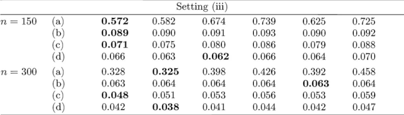
1000 runs there is some simulation uncertainty that leaves some of the comparisons still open and the identified 'winners' not quite clear.

wFIC pFIC wAIC pAIC wBIC pBIC

Setting (i) n

=

150 (a) 0.444 0.441 0.451 0.474 0.391 0.402 (b) 0.089 0.089 0.089 0.090 0.088 0.089 (c) 0.062 0.062 0.063 0.065 0.058 0.060 (d) 0.046 0.042 0.047 0.049 0.043 0.044 n

=

300 (a) 0.276 0.276 0.281 0.302 0.247 0.248 (b) 0.063 0.063 0.063 0.063 0.063 0.062 (c) 0.043 0.043 0.043 0.045 0.040 0.040 ( d) 0.034 0.031 0.034 0.036 0.032 0.032 Setting (ii) n

=

150 (a) 0.503 0.530 0.600 0.645 0.596 0.681 (b) 0.090 0.092 0.092 0.093 0.091 0.092 (c) 0.069 0.076 0.077 0.080 0.078 0.086 ( d) 0.062 0.056 0.060 0.063 0.064 0.072 n

=

300 (a) 0.304 0.315 0.364 0.383 0.368 0.430 (b) 0.063 0.064 0.064 0.064 0.064 0.064 (c) 0.047 0.051 0.052 0.054 0.053 0.059 (d) 0.041 0.037 0.041 0.043 0.043 0.048

Setting (iii) n = 150 (a) 0.572 0.582 0.674 0.739 0.625 0.725 (b) 0.089 0.090 0.091 0.093 0.090 0.092 (c) 0.071 0.075 0.080 0.086 0.079 0.088 (d) 0.066 0.063 0.062 0.066 0.064 0.070 n = 300 (a) 0.328 0.325 0.398 0.426 0.392 0.458 (b) 0.063 0.064 0.064 0.064 0.063 0.064 (c) 0.048 0.051 0.053 0.056 0.053 0.059 (d) 0.042 0.038 0.041 0.044 0.042 0.047

TABLE 9 .1. Root mean squared errors over 1000 simulation runs of the post model selection and model averaged estimators based on FIC, AIC and BIC for focus parameters

(a)

relative risk, (b) cumulative hazard, (c) survival probability and (d) median. Setting (i) corresponds to rJ = (0,0,0, O)t, (ii) to rJ = (3, -3,3, -3)t

and (iii) to rJ = (0,0,3, -3,3, -3)t.

In setting (i) the narrow model is the true model. It is known that the BIC is a consistent model selector and that it often works well for models with a small number of parameters. Hence it is expected to do well for this situation, as is indeed seen from the simulation results. It should be noticed that especially for focus parameters (b) and (d) the differences with the FIC values are only minor. For settings (ii) and (iii) where there are four more non-zero parameters in the true model than in the narrow model, BIC is no longer preferred. The smoothed FIC is clearly the best choice for setting (ii), where the wide model is true, while for the median as a focus point, the post-FIC selector gives the best results. The picture is more undecided for setting (iii) in between narrow and full model. For the smaller sample size for focus (c) the post-AIC gives the smallest simulated mse. Overall, model averaging tends to yield smaller simulated mse than post-model selection. Considering only the post-model selection estimators, we see that the pBIC performs well for the simplest setting where all extra parameters are zero. For setting

(ii)

the pFIC is the best, with the same conclusion for setting (iii), where all three criteria perform about equal for focus (b).

9.2. Survival analysis for malignant melanoma. Here we examine the data set de-scribed in Section 1. As already motivated, we include Xl in every model, and select

amongst the other variables Zl, . .. ,Z6 using an all subsets search. The seven hazard

re-gression coefficient estimates were 0.535 (0.277) for /31, 0.036 (0.052) for /1, 0.321 (0.192) for /2, -0.707 (0.314) for /3, -0.995 (0.324) for /4, 0.334 (0.241) for /5, 0.017 (0.008) for /6, with the estimated standard deviation (standard error) in parentheses, computed using the full model. In particular variables Xl, Z2, Z3, Z4, Z6 might be considered to have

a reasonably clear influence on life-times, as measured by the ratios estimate divided by standard error. Coefficients /1 and /5 would however not be seen as significantly different from zero in most analyses. We shall nevertheless see that variable Z5 often will be selected,

The model selection methods applied are AIC, BIC and four versions of FIC, each corresponding to a particular focus parameter. FI C 1 corresponds to /-Ll = exp{

(x - xo)

t

f3

+

(z - zo)t"(},

relative risk of a man, with average tumour thickness amongst all men partici-pating in the study, infection infiltration level Z2 = 3, epithelioid cells not present (Z3 = 2), ulceration present (Z4 = 1), invasion depth Z5 = 1, and average men's age in the study, as compared to that of women with averages of thickness of tumour and age computed over the subgroup of women in the study, and the other covariates remaining the same. The first set of covariates for men defines the variables level

(x, z),

while the second set corresponds to

(xo, zo).

FIC2 computes the FIC values for /-L2 =

Ho(t)

at time

t

= 1584 days which corresponds to the time where the estimated Kaplan-Meier survival probability reaches 0.85. The third focus, which defines FIC3, is the survival probability at time

t

= 1584 for the same set of covariates

(x, z)

as for the first focus parameter, i.e. /-L3 = Su(t I

x, z).

The final focus parameter is /-L4 = ~(0.10) = Su-1_{(0.90 I}

_x,z),

_{the time at which at least 90% of} the patients with covariate level

(x, z)

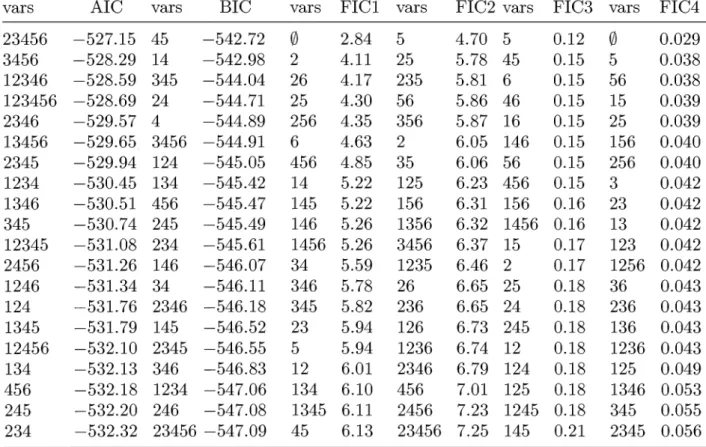
are still alive.

Table 9.2 shows the 20 highest ranked score values for each of the criteria in question, after having searched through all 26 _{= 64 candidate models, along with the selected Zj}

variables; '245' means that variables Z2, Z4, Z5 are included, etc. Note that the values are

sorted in importance per criterion.

vars AIC vars BIC vars FICI vars FIC2 vars FIC3 vars FIC4 23456 -527.15 45 -542.72

0

2.84 5 4.70 5 0.12

0

0.029 3456 -528.29 14 -542.98 2 4.11 25 5.78 45 0.15 5 0.038 12346 -528.59 345 -544.04 26 4.17 235 5.81 6 0.15 56 0.038 123456 -528.69 24 -544.71 25 4.30 56 5.86 46 0.15 15 0.039 2346 -529.57 4 -544.89 256 4.35 356 5.87 16 0.15 25 0.039 13456 -529.65 3456 -544.91 6 4.63 2 6.05 146 0.15 156 0.040 2345 -529.94 124 -545.05 456 4.85 35 6.06 56 0.15 256 0.040 1234 -530.45 134 -545.42 14 5.22 125 6.23 456 0.15 3 0.042 1346 -530.51 456 -545.47 145 5.22 156 6.31 156 0.16 23 0.042 345 -530.74 245 -545.49 146 5.26 1356 6.32 1456 0.16 13 0.042 12345 -531.08 234 -545.61 1456 5.26 3456 6.37 15 0.17 123 0.042 2456 -531.26 146 -546.07 34 5.59 1235 6.46 2 0.17 1256 0.042 1246 -531.34 34 -546.11 346 5.78 26 6.65 25 0.18 36 0.043 124 -531.76 2346 -546.18 345 5.82 236 6.65 24 0.18 236 0.043 1345 -531.79 145 -546.52 23 5.94 126 6.73 245 0.18 136 0.043 12456 -532.10 2345 -546.55 5 5.94 1236 6.74 12 0.18 1236 0.043 134 -532.13 346 -546.83 12 6.01 2346 6.79 124 0.18 125 0.049 456 -532.18 1234 -547.06 134 6.10 456 7.01 125 0.18 1346 0.053 245 -532.20 246 -547.08 1345 6.11 2456 7.23 1245 0.18 345 0.055 234 -532.32 23456 -547.09 45 6.13 23456 7.25 145 0.21 2345 0.056

TABLE 9.2. Values of the information criteria AIC, BIC and FIC for four focus parameters: (1) relative risk, (2) cumulative hazard, (3) survival probability, and

(4) 10% quantile ~(0.10)

=

Su-1 _{(0.90). The table shows the 20 largest AIC}