Air Force Institute of Technology
AFIT Scholar
Theses and Dissertations Student Graduate Works
6-13-2013
The Dynamic Multi-objective Multi-vehicle
Covering Tour Problem
Joshua S. Ziegler
Follow this and additional works at:https://scholar.afit.edu/etd
Part of theComputer Sciences Commons
This Thesis is brought to you for free and open access by the Student Graduate Works at AFIT Scholar. It has been accepted for inclusion in Theses and Dissertations by an authorized administrator of AFIT Scholar. For more information, please [email protected].
Recommended Citation
Ziegler, Joshua S., "The Dynamic Multi-objective Multi-vehicle Covering Tour Problem" (2013).Theses and Dissertations. 913.
THE DYNAMIC MULTI-OBJECTIVE MULTI-VEHICLE COVERING TOUR PROBLEM
THESIS
Joshua S. Ziegler, AFIT-ENG-13-J-09
DEPARTMENT OF THE AIR FORCE AIR UNIVERSITY
AIR FORCE INSTITUTE OF TECHNOLOGY
Wright-Patterson Air Force Base, OhioDISTRIBUTION STATEMENT A:
The views expressed in this thesis are those of the author and do not reflect the official policy or position of the United States Air Force, the Department of Defense, or the United States Government.
This material is declared a work of the U.S. Government and is not subject to copyright protection in the United States.
AFIT-ENG-13-J-09
THE DYNAMIC MULTI-OBJECTIVE MULTI-VEHICLE COVERING TOUR PROBLEM
THESIS
Presented to the Faculty
Department of Electrical and Computer Engineering Graduate School of Engineering and Management
Air Force Institute of Technology Air University
Air Education and Training Command in Partial Fulfillment of the Requirements for the Degree of Master of Science in Computer Science
Joshua S. Ziegler, B.S.
June 2013
DISTRIBUTION STATEMENT A:
AFIT-ENG-13-J-09
THE DYNAMIC MULTI-OBJECTIVE MULTI-VEHICLE COVERING TOUR PROBLEM
Joshua S. Ziegler, B.S.
Approved:
/signed/
Gilbert L. Peterson, PhD (Chairman)
/signed/ Gary B. Lamont, PhD (Member)
/signed/
Maj Kennard R. Laviers, PhD (Member)
21 May 2013 Date 21 May 2013 Date 21 May 2013 Date
AFIT-ENG-13-J-09
Abstract
This work introduces a new routing problem called the Dynamic Mulit-Objective Multi-vehicle Covering Tour Problem (DMOMCTP). The DMOMCTPs is a combinatorial optimization problem that represents the problem of routing multiple vehicles to survey an area in which unpredictable target nodes may appear during execution. The formulation includes multiple objectives that include minimizing the cost of the combined tour cost, minimizing the longest tour cost, minimizing the distance to nodes to be covered and maximizing the distance to hazardous nodes. This study adapts several existing algorithms to the problem with several operator and solution encoding variations. The efficacy of this set of solvers is measured against six problem instances created from existing Traveling Salesman Problem instances which represent several real countries. The results indicate that repair operators, variable length solution encodings and variable-length operators obtain a better approximation of the true Pareto front.
Table of Contents
Page
Abstract . . . iv
Table of Contents . . . v
List of Figures . . . viii
List of Tables . . . ix
List of Symbols . . . x
List of Acronyms . . . xii
I. Introduction . . . 1 1.1 Contributions . . . 2 1.2 Background . . . 2 1.3 Methodology . . . 2 1.4 Limitations of Study . . . 3 1.5 Outline . . . 4 1.6 Summary . . . 4
II. Problem Definition . . . 5
III. Background . . . 9
3.1 Problem Objectives . . . 9
3.1.1 Multiple Objectives . . . 9
3.1.2 Solving Multiobjective Problems . . . 11
3.1.3 Decision Maker . . . 12
3.1.4 A posteriori Performance Measures . . . 12
3.1.4.1 Hypervolume . . . 13
3.1.4.2 Generational Distance . . . 14
3.1.4.3 Generalized Spread . . . 14
3.1.4.4 Constraints Violated . . . 15
3.2 Related Problems . . . 15
3.2.1 Base Routing Problem (the Traveling Salesman Problem) . . . 16
3.2.2 Covering Constraints . . . 17
Page
3.2.3 Dynamic Problem Variants . . . 20
3.2.3.1 Dynamic Demand for Known Customers . . . 21
3.2.3.2 Adding Previously Unknown Customers . . . 22
3.2.3.3 Dial a Ride/Flight Problem . . . 23
3.2.3.4 Dynamic Traveling Salesman Problem . . . 24
3.2.3.5 Dynamic Traveling Repairperson Problem . . . 25
3.2.4 Multiple Objective Variations . . . 27
3.2.5 Multiple Vehicles . . . 27
3.3 Solution Methods . . . 28
3.3.1 Exact Methods . . . 28
3.3.2 Heuristics . . . 29
3.3.2.1 Extracting Most Likely State . . . 30
3.3.2.2 Robust Control . . . 30
3.3.2.3 Potential Field Control . . . 31
3.3.2.4 Reactive Control . . . 32
3.3.2.5 Reinforcement Learning . . . 32
3.3.3 Metaheuristics . . . 33
3.4 Summary . . . 34
IV. Methodology . . . 35
4.1 Native Problem Domain . . . 35
4.2 Native to Model Problem Domain Mapping . . . 35
4.2.1 Vehicle Model . . . 36 4.2.2 Time Model . . . 37 4.2.3 Problem Instances . . . 37 4.2.3.1 Dynamism . . . 38 4.2.3.2 Unit Adaptations . . . 38 4.2.4 Decision Maker . . . 39 4.3 Simulation Execution . . . 41 4.3.1 High-Level Design . . . 41 4.3.2 Implementation . . . 42 4.3.3 Implementation Limitations . . . 43 4.4 Performance Measures . . . 43 4.5 Solvers Studied . . . 44 4.5.1 Solution Types . . . 45 4.5.2 Operators . . . 46 4.5.2.1 Initialization . . . 47 4.5.2.2 Selection . . . 47 4.5.2.3 Crossover . . . 47 4.5.2.4 Mutation . . . 48
Page 4.5.3 Parameters . . . 50 4.5.4 Algorithms Tested . . . 51 4.6 Summary . . . 53 V. Results . . . 54 5.1 Data Presentation . . . 54 5.2 Data . . . 55 5.3 Algorithm-Level Analysis . . . 67 5.4 Operator-Level Analysis . . . 70 5.5 Summary . . . 71 VI. Conclusion . . . 74 6.1 Results . . . 75 6.2 Significance of Study . . . 75 6.3 Limitations of Study . . . 75 6.4 Future Work . . . 76 6.5 Summary . . . 76
Appendix A: Violin Plots . . . 78
Appendix B: Pareto Front Plots . . . 112
List of Figures
Figure Page
2.1 Third Objective Example. . . 5
2.2 Covering Unvisitable Nodes. . . 6
3.1 Pareto Dominance. . . 10
3.2 Pareto Front. . . 11
3.3 Hypervolume Example for Two Objectives. . . 13
3.4 DMOMCTP relations to the m-CTP, CTP and TSP. . . 15
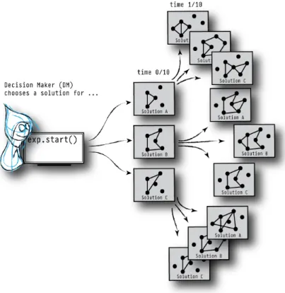
4.1 Decision Maker Process. . . 36
4.2 Decision Maker Process att1. . . 41
4.3 Experiment Execution. . . 43
5.1 Uruguay 734 - Light EDOD - Violin Plots . . . 56
5.2 Uruguay 734 - Light EDOD - Pareto Fronts . . . 57
5.3 Uruguay 734 - Moderate EDOD - Violin Plots . . . 58
5.4 Uruguay 734 - Moderate EDOD - Pareto Fronts . . . 59
5.5 Canada 4663 - Light EDOD - Violin Plots . . . 60
5.6 Canada 4663 - Light EDOD - Pareto Fronts . . . 61
5.7 Canada 4663 - Moderate EDOD - Violin Plots . . . 62
5.8 Canada 4663 - Moderate EDOD - Pareto Fronts . . . 63
5.9 USA 13509 - Light EDOD - Violin Plots . . . 64
5.10 USA 13509 - Light EDOD - Pareto Fronts . . . 65
5.11 USA 13509 - Moderate EDOD - Violin Plots . . . 66
List of Tables
Table Page
2.1 DMOMCTP Objectives. . . 7
3.1 Common routing problem elements. . . 17
3.2 Dynamic Traveling Repairperson Problem (DTRP) Policies Proposed by Bertsimas and Van Ryzin. . . 25
3.3 Common solution methods for routing problems. . . 29
4.1 Algorithm, Solution Type and Operator Incompatibilities. . . 46
4.2 Monolithic Repair Operator Flags. . . 49
4.3 Algorithm Paramaters. . . 51
List of Symbols
Symbol Definition
c covering distance
Ccapacity capacity for each vehicle, given as a scalar or vector when using multiple goods
di demand for nodevi ∈V; can be a scalar or vector when using multiple goods
D vector of demands for all nodes∀vi ∈V∃di ∈D
e(i,j) member ofE- cost from nodevitovj
E matrix of least cost paths from any node to any other node fi(R) objective functioniw.r.t. R
G graph
ki vehiclei;ki ∈K
K set of vehicles
L maximum length of each vehicle route (assuming constant, identical speed; speed and cost condidered interchangable)
mi time slicei;mi ∈M
M set of time slices
O set of nodes that cannot be visited
P subset of customersVthat may demand goods later on (as in the Dynamic Travelling Salesman Problem)
ri routei;ri ∈R
R set of all routes
T set of nodes that must be visited
v0 depot - starting and ending point of all vehicles (unless specified otherwise)
Symbol Definition
List of Acronyms
Acronym Definition
AbYSS Archive-based Scatter Search ACO Ant Colony Optimization
ADP Approximate Dynamic Programming AI Artificial Intelligence
AUV Autonomous Underwater Vehicle CLP Clover Leaf Problem
CSP Covering Salesman Problem CTP Covering Tour Problem
CVRP Capacitated Vehicle Routing Problem DAFP Dial-A-Flight-Problem
DARP Dial-A-Ride-Problem
DC Divide and Conquer
DM decision maker
DMOMCTP Dynamic Mulit-Objective Multi-vehicle Covering Tour Problem
DOD Degree of Dynamism
DREP Distributed Resource Exploitation Problem DTRP Dynamic Traveling Repairperson Problem DTSP Dynamic Traveling Salesman Problem EDOD Effective Degree of Dynamism
EPCA Exponential family Principal Components Analysis FCFS First Come First Serve
GIS Geographic Information System
Acronym Definition
LW Center-of-Gravity Longest Wait mCTP multi-vehicle Covering Tour Problem MDP Markov decision process
mDTRP multi-vehicle Dynamic Traveling Repairperson Problem MOEA Multiobjective Evolutionary Algorithm
MOP Multiobjective Problem
MOGA Multi-Objective Genetic Algorithm mSQM multi-vehicle Stochastic Queue Mediam
mTSPTW multi-Travelling Salesman Problem with Time Windows NDP Neuro-Dynamic Programming
NSGA Nondominated Sorted Genetic Algorithm NSGA-II Nondominated Sorted Genetic Algorithm II
NN Nearest Neighbor
NNRW Nearest Neighbor with Random Weights OP Orienteering Problem
PACO Parallel Ant Colony Optimization PAES Pareto Archived Evolution Strategy PDP Pickup and Delivery Problem
PDTRP Partially Dynamic Travling Repairman Problem POMDP partially observable Markov decision process PPP Persistent Patrolling Problem
SPEA Strength Pareto Evolutionary Algorithm SPEA2 Strength Pareto Evolutionary Algorithm 2 RBX Route Based Crossover
Acronym Definition
RP Random Process
RS Random Search
RV Random Variable
RVRP Robust Vehicle Routing Problem SBRP School Bus Routing Problem SBX Simulated Binary Crossover TSP Traveling Salesman Problem UAV Unmanned Aerial Vehicle
USBRP Urban School Bus Routing Problem VEGA Vector Evaluated Genetic Algorithm VRP Vehicle Routing Problem
THE DYNAMIC MULTI-OBJECTIVE MULTI-VEHICLE COVERING TOUR PROBLEM
I. Introduction
Field intelligence quality and timeliness can be instrumental in war and peace. Recent advances in Unmanned Aerial Vehicles (UAVs) have provided an exciting new avenue for collecting that intelligence without risk to pilots. By allocating several UAVs to a given mission - cooperating as a swarm - mission time can be reduced. Planning such missions is a difficult problem however. The time required, unknown information, distance to surveillance targets, and distance to known hostile forces need to be considered. In order to study this problem, it must first be defined mathematically. This work uses the existing Covering Tour Problem (CTP) [65] as a starting point.
The CTP is a routing problem where a single vehicle must visit a subset of all the points provided while covering another subset [65]. In this context, the vehicle must visit some pointAwithin a predefined distance of the node Bto “cover” it. The objective is to minimize the cost of the route while abiding by these constraints. This basic formalizations can then be modified in order to study a number of real-world problems such as mobile medical unit routing [49, 78], school bus routing [124] and dial-a-ride routing [154].
This work takes the multi-vehicle Covering Tour Problem (mCTP) [73] variation of the CTP as a starting point because no existing variations of it - or any other routing problem - fit the native UAV problem described above. Namely, no existing problem exists that simultaneously provides dynamically revealed nodes, nodes to be avoided, covering constraints, multiple vehicles, and objectives to minimize the combined route cost, minimize the wall-clock time taken, maximized the combined distance to all nodes to avoid
and minimize the combined distance to all nodes to be covered. This work introduces such a problem formalization and studies a set of solution methods in an a posteriori fashion.
1.1 Contributions
This work introduces a novel CTP formalization - the Dynamic Mulit-Objective Multi-vehicle Covering Tour Problem (DMOMCTP) - which includes additional objectives and unknown nodes that appear during execution. The goal of the work is to find the best set of centralized solvers and operators from the tested set for the DMOMCTP. This allows future works to focus on promising algorithms while including the best from this work for comparison. This work also provides insight into operator design with respect to the DMOMCTP.
1.2 Background
Dozens of routing problem formalizations exist with varying constraints and objectives. While none of the individual components of the problem are unique, the combination presented here represents a new formalization. This work briefly reviews a number of related works on problems and their solution methods ranging from the Traveling Salesman Problem (TSP) [149] to the multi-vehicle Covering Tour Problem (mCTP).
1.3 Methodology
This work approaches the DMOMCTP from an a posteriori perspective, meaning that the result of any solver is a set of solutions. Furthermore, each solver is given three minutes to find the best solution set it can, as opposed to a set number of iterations. This models the time requirements of a real UAV system. Algorithms tested include Nearest Neighbor with Random Weightss (NNRWs), Archive-based Scatter Searchs (AbYSSs), Strength Pareto Evolutionary Algorithm 2 (SPEA2), Nondominated Sorted Genetic Algorithm II (NSGA-II) and Random Search (RS). Modified versions of these algorithm are also
included, which replace the operators and/or solution encoding of the base algorithm. Operators used include Simulated Binary Crossovers (SBXs), Route Based Crossovers (RBXs), Uniform addition, Uniform deletion, and monolithic repair. Solution encodings include fixed and variable length.
As is common to studies of this nature, the quality of these sets are assessed via several metrics [38]. This work uses hypervolume, generalized spread, and number of constraints violated. This complicates analysis because unlike single-objective studies, the best is subjective. The best ultimately relies on the preferences of the user. For example, a solver may have the best hypervolume values, but worst constraints violated values. Finally, although the multiobjective nature of the results and No Free Lunch Theorem limits the conclusions we can make from such experimentation, a rough ordering of the solvers tested is provided.
1.4 Limitations of Study
The native problem domain is inherently complex and difficult to solve which was the impetus for limiting the formalization’s scope. Issues related to real-world problems such as navigation, communication, and physics are removed and left for later works. The resulting formalization is still an interesting and difficult problem that provides a stepping stone to more complete problems. Specifically, we have chosen to focus on central solvers which provide a solution baseline for future work.
Note that, this work only provides results for fifty independent runs for each algorithm over six problem instances - largely due to the real-world time required for computation. As in other Multiobjective Problems (MOPs) the nature of this problem and low number of data points, the resulting data is not normal. The problem instances themselves are taken from real-world Geographic Information System (GIS) data sets, but the nodes are assigned to the various sets using a Uniform Random Variable (RV) which is an assumption that may not hold in all problem instances.
1.5 Outline
Chapter 2 introduces a formal version of the native problem: the DMOMCTP. Chapter 3 reviews the routing problem literature from the computer science, operations research, and robotics communities. The DMOMCTP is shown to reduce to the TSP, making the DMOMCTP NP-complete. Chapter 4 defines the experiment, including the data and metrics chosen to measure algorithm efficacy with respect to the DMOMCTP. Chapter 5 provides and discusses the results.
1.6 Summary
Motivated by a complex, multiobjective, multivehicle routing problem with covering constraints this work introduces a new formalization - the DMOMCTP. Related works from routing problems, Artificial Intelligence (AI), and MOPs are discussed briefly. As a new problem formalization and given the No Free Lunch Theorem, these works provide limited value in solving this problem. Thus the purpose of this work is to study several centralized solvers against the DMOMCTP and provide a reduced set to recommend for future works and applications. Given the limited number of problem instances and independent runs, the work finds four promising algorithms including two versions of both NSGA-II and SPEA2. It then discusses the possible reasons for these results and future directions for research.
II. Problem Definition
T
his chapter introduces the unique problem domain - the Dynamic Mulit-ObjectiveMulti-vehicle Covering Tour Problem (DMOMCTP) - to provide context before discussing related work in Chapter 3. While the DMOMCTP is related to other vehicle tour problems it differs in several details resulting in a fundamentally different problem.
v
0∈
V
v
1∈
T
v
2∈
W
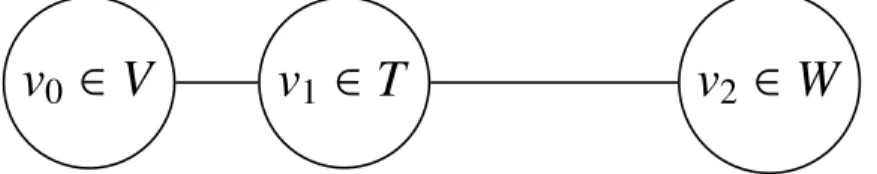
Figure 2.1: Third Objective Example.
Given an undirected graph G = (Vall,E) where {v0,vi, . . . ,vj} ∈ Vall is the set of
all nodes. E is a matrix representing the cost to travel between any two nodes such that
∃e(i,j) ∈ E ∀vi,vj ∈ V; e(i,j) ∈ R ≥ 0; i , j. The e(i,j) costs denote the cheapest path
between any two nodes and not that the graph is fully-connected. This makes E a lossy representation of the true graph. The edges in the original undirected graph are symmetrical and satisfies the triangle inequality.
The nodes inVallcan belong to one or more of three sets:W,T andOwhich represent the nodes which must be covered (W), must be visited (T) and cannot be visited (O). The only restriction on set assignment is that nodes cannot belong to T andOsimultaneously which would render the problem infeasible. Covering a nodevi ∈ W requires at least one
vehiclekn ∈ K to visit a nodevj ∈ V;vj < Owithin a preset distancecof the node to be
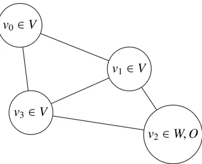
v
0∈
V
v
1∈
V
v
3∈
V
v
2∈
W
,
O
Figure 2.2: Covering Unvisitable Nodes.
The goal is to find a set of routes R (e.g. r0 = {v0,v5,v2,v0} ∈ R) for K identical
vehicles with infinite capacity, where|R| = |K|, to visit all nodes inT and cover all nodes inW without visiting any inO. All routes must begin and end at a preset nodev0called the
depot. Nodes can be visited any number of times by any number of vehicles.
Further complicating matters, the environment is dynamic in that previously unknown nodes are added to the graph as time progresses (i.e. environment is partially observable). These nodes are immediately assigned to their appropriate subsets (i.e.W, T, O). Nodes never disappear once known. The problem can be resolved after each after each state update, referred to as a time slicemi ∈ M. Each time slice can be thought of as a static
problem instance, however the vehicles K may start at any nodevi ∈ Vall;vi <Oand may
be between nodes.
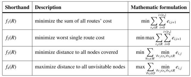
The resulting set of routes R must meet the four objectives listed in Table 2.1. The first objective - f1(R) - is to minimize the combined cost of all routes (e.g. if cost is related
Table 2.1: DMOMCTP Objectives.
Shorthand Description Mathematic formulation
f1(R) minimize the sum of all routes’ cost min
X rn∈R i<|rn| X i=0 ei,i+1
f2(R) minimize worst single route cost min max
X rn∈R i<|rn| X i=0 ei,i+1
f3(R) minimize distance to all nodes covered min
X
∀vi∈W
min
∀vj∈rn∀rn∈R
ei,j
f4(R) maximize distance to all unvisitable nodes max
X
∀vi∈O
min
∀vj∈rn∀rn∈R
ei,j
(f2(R)) - minimize the worst route’s cost - minimizes the cost of the entire solution when
treating each vehicle as independent (e.g. if edge cost represents time, this minimizes the time taken to complete the problem). The third objective (f3(R)) seeks to minimize the
distance between each node to be covered and the closest visited node among all routes. This acts as an attractive force on the vehicle (e.g. if the nodes in W represent areas of interest to be investigated using on board sensors with a maximum range ofcthis increases the quantity of that sensor data).
For example, consider Figure 2.1. If v0 is the depot, we could simply visit v1
and meet the requirements (assuming the covering distance c is large enough to reach v2). However f3(R) would equal the cost of e(v1,v2). If we instead visit both v1 and
v2, f3(R) = 0. This does increase the evaluation of the first two objective functions
(f1(v0,v1,v2,v1,v0)> f1(v0,v1,v0) and similarly for f2(R)). Alternatively nodes may require
a vehicle to cover them but cannot be visited (i.e.vi ∈W andvi ∈O) as in Figure 2.2 with
v2(in these cases, f3(R) cannot be minimized to 0).
The fourth objective (f4(R)) is to maximize the distance between each node visited
represent hostile forces such as anti-aircraft installations, this reduces the risk our vehicles face).
III. Background
T
he Dynamic Mulit-Objective Multi-vehicle Covering Tour Problem (DMOMCTP)is composed of several components: dynamic nodes, multiple objectives, covering constraints and route planning. This chapter reviews previous work in these areas starting with the basic differences between single and Multiobjective Problems (MOPs). It briefly touches on basic solution methods and performance measures for each. It then proceeds to problem formulations, both single and multiobjective, which are related to the DMOMCTP. The final section of the chapter revisits solution methods, considering their pros, cons and past applications.
3.1 Problem Objectives
Problems can be split into two categories: single and multiobjective. Single objective problems determine the utility of their solutions with a single measure. For the Traveling Salesman Problem (TSP), the objective is to find the shortest route visiting each city exactly once and ending at the starting point. The utility of a TSP solution is its length. Single objectives problems can be defined mathematically as minimizing (or maximizing) the utility defined by some function f(x) where x is the vector of decisions variables (x= (x1, . . . ,xn)) subject to any constraints. A constraint is any limitation on any decision
variable(s) (i.e. the domain of the variable). For example, the TSP has the constraint that ”each city may only be visited once.”
3.1.1 Multiple Objectives.
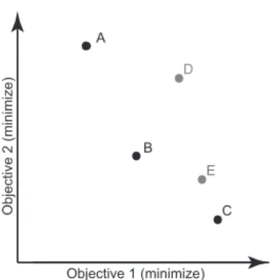
Multiobjective problems differ in that their utility is defined as a vector. For example, if the TSP is modified to include multiple salesmen it may be desirable to minimize the variance among the assigned routes. Each solution’s utility is then defined as a vector f(x) = (k1,k2) which can be visualized in a two-dimensional objective space as
in Figure 3.1. Now consider two solutions: s1 = (10,1) and s2 = (8,2). Each solution is
better than the other with respect to at least one objective meaning there is no single best [38]. The result from a MOP solver is asetof solutions.
A D E A D E A Objective 1 (minimize) O b je ct ive 2 (mi n imi ze )
Figure 3.1: Pareto Dominance.
Formally, a solution si is said to weakly dominate another sj if it has at least one
objective k ∈ K that is better than sj’s and is at least equal to sj in all other objectives: ∀k ∈ {1, . . . ,k}, f(si)k ≤ f(sj)k ∧ ∃l ∈ {1, . . . ,k} | f(si)l < f(sj)l [38]. A solutionsi is said
tostronglydominate another sj if it improves upon all objectives: ∀k ∈ {1, . . . ,k}, f(si)k <
f(sj)k. For example, solution A strongly dominates both Dand E in Figure 3.1 because
all of its objectives are better than theirs. More generally,Awould strongly dominate any solutions in the light gray box. SolutionAis said to be non-dominated.
The set of solutions which are not strongly dominated (but may be weakly-dominated) is known as the Pareto front, which is a subset of the entire solution set. For example, solutionsA,B,andCin Figure 3.2 are non-dominated and form the Pareto front out of the solution setS = {A,B,C,D,E}. For every MOP, there exists a Pareto front known as Ptrue
which is the best possible set of non-dominated solutions. Typically this set is infeasible to compute and can only be approximated [38]. This approximated Pareto front is the best
A B C D E Objective 1 (minimize) O b je ct ive 2 (mi n imi ze )
Figure 3.2: Pareto Front.
3.1.2 Solving Multiobjective Problems.
Algorithms for solving multiobjective problems are categorized here into two groups: deterministic and stochastic solvers. Enumerative methods are a special type of deterministic method. Enumerative methods are those which evaluate all possible solutions given the problem constraints [38]. These methods are simple to implement and understand but become impractical when the search space becomes large [38].
Other deterministic methods exist which exploit domain knowledge in the form of heuristics to circumvent the search space explosion [14]. Examples include greedy search, hill-climbing and branch and bound. However, real-world MOPs are “high-dimensional, discontinuous, multimodal, and/or NP-Complete . . . problems exhibiting one or more of these above characteristics are termed irregular. Because many real-world scientific and engineering MOPs are irregular, enumerative and deterministic search techniques are then unsuitable” [38].
Stochastic algorithms form the second type of algorithms. Examples include simulated annealing, Monte Carlo simulation and evolutionary computation. This class of algorithms use random decisions in an attempt to approximate the best solution(s). Perhaps the most basic stochastic algorithm is a random walk. In a TSP instance, a Random Variable (RV) would iteratively choose the next node to visit and remove it from the list
of candidates. A Random Variable (RV) is a value is decided by chance in a mathematical sense. That is, it does not have a set value. When the list of candidates is empty the solution is evaluated and the process restarts. Many stochastic algorithms use problem domain-specific heuristics or operators to guide their search to strategically search the space.
3.1.3 Decision Maker.
Since multiobjective problem solvers result in a set of solutions, there must be a human decision maker (DM) to choose “the best” [38]. This can be done one of two ways: a priori or a posteriori.
A priori methods require the human DM to choose a method of combining the objectives into one [38]. There are several ways to do this, perhaps the simplest of which is to create a weighted combination function (e.g. f(s) = a· f1(s)b+· · ·+c· fk(s)d) [38].
The multiobjective problem can then be treated as single objective.
A posteriori methods require a human DM to choose a solution from the set. The objectives are not altered or combined leaving the DM to determine which trade offs are best [38].
A priori methods are desirable for their relative simplicity. However, human DM preferences are difficult to define mathematically, or are problem dependent in practice [38]. A posteriori methods are simple in theory, but presenting the solutions to the human DM can be a difficult data visualization problem in itself [26].
3.1.4 A posteriori Performance Measures.
Since a posteriori solvers produce a set of solutions, the quality of that set must be measured. Desirable qualities of a solution set include the degree to which it approximates Ptrue and the spread or variety of the solutions along the Pareto front [38]. As discussed
above, Ptrue can be infeasible to compute, so many a posteriori multiobjective works
aggregating all non-dominated solutions from all algorithms and represents the best known Pareto front [38]. The following sections briefly cover several metrics.
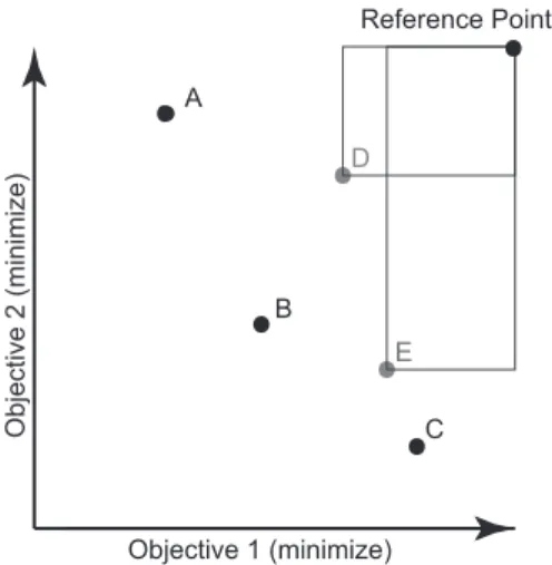
3.1.4.1 Hypervolume.
HV={[ i
areai |veci ∈ Pknown} (3.1)
Hypervolume is a metric that measures the volume represented by all of a set’s members in n-dimensional objective space (i.e. hyperspace) [38]. This can be provided as a ratio of Pknown’s hypervolume. A solution set’s hypervolume is the summation of all
of the hypercubes’ volume. These shapes are bounded by each solution’s fitness and an arbitrary boundary point (e.g. the worst solution) in objective space [38]. The formula for hypervolume is shown in Equation (3.1) where “veci is a non-dominated vector in Pknown
and areai is the area between the origin and vector veci[38]. If the front of non-dominated
solutions is not convex, the resulting hypervolume may be misleading [38]. This metric is to be maximized and provides a sense of the sets goodness, but not its diversity [38]. A hypervolume ratio of 1 would mean that the set fills up a space as great as the known Pareto front. A B C D E Objective 1 (minimize) O b je ct ive 2 (mi n imi ze ) Reference Point
Figure 3.3 presents a two dimensional example. The points A through E represent solutions A through E in objective space. If Algorithm A produces the non-dominated set (D,E) its hypervolume would be calculated by first choosing a reference point (see top right) and then calculating the area covered by the bounding boxes from each point to the reference point. This combined area is the hypervolume of algorithm A’s non-dominated solution set. Repeating this process for the known Pareto front, we then come up with the ratio of algorithm A’s hypervolume to the known Pareto front (0≤ HV ≤1).
3.1.4.2 Generational Distance. GD= ( Pn i=1d p i) 1 p |PFknown| (3.2) Generational distance - see Equation (3.2) - is a measure of the average distance between a non-dominated set’s members and those of the known Pareto front in objective space (n-dimensional) [38]. PFknown is “the number of vectors in PFknown, p = 2, and di
is the Euclidean phenotypic distance between each member, i, of PFknown and the closest
member in PFtrue to that member.” In our experiment, PFknown is the non-dominated set
from an algorithm, andPFtrueis the non-dominated set of solutions created by aggregating
all solutions from all runs and algorithms which we refer to asPknown. This metric is to be
minimized.
3.1.4.3 Generalized Spread.
Generalized spread measures the distance from a given point to its nearest neighbor. This measure was introduced by Durillo and Nebro [52] as a replacement for the spread metric which only works in 2-dimensional space. Mathematically:
Spread= m P i=1 d(ei,S)+ P X∈S |d(X,S)−d¯| m P i=1 d(ei,S)+|S| ∗d¯ (3.3)
where “S is a set of solutions, S∗is the set of Pareto optimal solutions (e1, . . . ,em) are m
extreme solutions inS∗,mis the number of objectives and”
d(X,S)= min Y∈S,Y,X||F(X)−F(Y)|| 2 (3.4) ¯ d= 1 |S∗| P X∈S∗ d(X,S) (3.5)
Generalized spread measures the diversity of the solutions set and is to be minimized.
3.1.4.4 Constraints Violated.
Number of constraints violated is not a MOP specific metric, but provides an important measure of solution feasibility for constrained problems like the DMOMCTP. This is useful because many algorithms allow for infeasible solutions in an attempt to circumvent local optima to find global optima. The calculation of violated constraints is problem domain specific. This metric is to be minimized.
3.2 Related Problems
The DMOMCTP is, at its core, a routing problem. Given the popularity and numerous variations of such problems, the body of previous work is expansive (especially in the operations research community) [42]. Since the DMOMCTP is a new problem formulation we briefly review a broad range of related works. Particular focus is placed on the multi-vehicle Covering Tour Problem (mCTP), Covering Tour Problem (CTP) and TSP, which are the most closely related problem formulations.
DMOMCTP
f1(R) only,|M|= 1,O=∅mCTP
|K|=1CTP
W = ∅TSP
To understand why the focus is placed on these three problems, this section briefly outlines their relation to the DMOMCTP informally (shown in Figure 3.4). Ignoring the dynamic and multi-objective elements of the DMOMCTP (i.e. using f1(R) from Table 2.1
for our singular objective) we are left with the mCTP. Utilizing only one vehicle in that problem reduces it to the CTP. Removing the covering constraint from the CTP reduces the problem to the TSP. Thus the DMOMCTP is related to these three problems which explains our detailed coverage. Works that differ in more significant ways (e.g. such as changing the objective function) are covered in less detail, relying instead on applicable reviews when possible.
The most basic formulations of these problems - as indicated above - have been static, deterministic, single-objective versions of the TSP, CTP and Vehicle Routing Problem (VRP). Reviews of work in this area include [16, 39, 89, 90]. Recent developments enabling real-time communication, global positioning and re-routing has resulted in research in dynamic, partially-observable and stochastic variations of these problems [42, 66, 126]. Given the rise in unique problem formulations and complex relations between them, we have broken out many of the constraints and characteristics associated with each variation in Table 3.1. The sections that follow review these elements and the problems that include them.
3.2.1 Base Routing Problem (the Traveling Salesman Problem).
Possibly the most well-known of routing problems is the TSP [55, 149]. Given a graph G = (V,E) where V are the nodes and E the matrix of edge costs, the problem is to find the shortest path originating at the depot, visiting all cities (i.e.∀vi ∈V) and then returning
to the depot. Lawler, et al. [94] provides an extensive overview of the TSP. The problem was shown to be NP-hard by Karp [87]. This is important because it forms a special case of the DMOMCTP where there is only one vehicle (|K| = 1), no nodes to cover (W = ∅), no nodes that cannot be visited (O = ∅), only one time slice|M|= 1, all nodes belong to
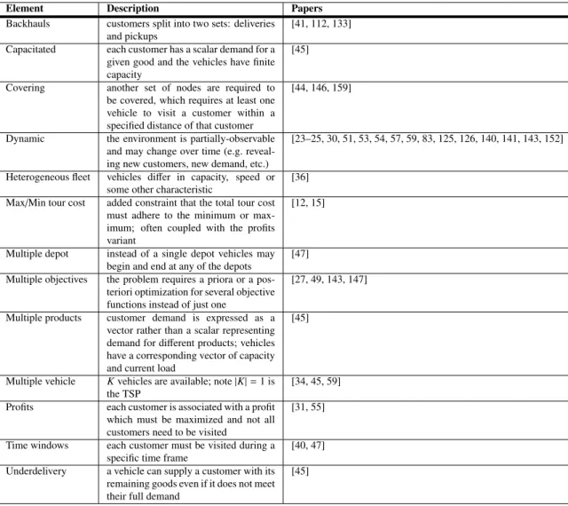
Table 3.1: Common routing problem elements.
Element Description Papers
Backhauls customers split into two sets: deliveries and pickups
[41, 112, 133] Capacitated each customer has a scalar demand for a
given good and the vehicles have finite capacity
[45]
Covering another set of nodes are required to be covered, which requires at least one vehicle to visit a customer within a specified distance of that customer
[44, 146, 159]
Dynamic the environment is partially-observable and may change over time (e.g. reveal-ing new customers, new demand, etc.)
[23–25, 30, 51, 53, 54, 57, 59, 83, 125, 126, 140, 141, 143, 152]
Heterogeneous fleet vehicles differ in capacity, speed or some other characteristic
[36] Max/Min tour cost added constraint that the total tour cost
must adhere to the minimum or max-imum; often coupled with the profits variant
[12, 15]
Multiple depot instead of a single depot vehicles may begin and end at any of the depots
[47] Multiple objectives the problem requires a priora or a
pos-teriori optimization for several objective functions instead of just one
[27, 49, 143, 147]
Multiple products customer demand is expressed as a vector rather than a scalar representing demand for different products; vehicles have a corresponding vector of capacity and current load
[45]
Multiple vehicle Kvehicles are available; note|K|=1 is the TSP
[34, 45, 59] Profits each customer is associated with a profit
which must be maximized and not all customers need to be visited
[31, 55]
Time windows each customer must be visited during a specific time frame
[40, 47] Underdelivery a vehicle can supply a customer with its
remaining goods even if it does not meet their full demand
[45]
the must visit set (T ⊆ V) and only f1(R) is used (single objective). Thus, the DMOMCTP
is also at least NP-hard and solution methods for the TSP may show promise when adapted to the DMOMCTP. Especially when considering works that capture more elements of the DMOMCTP (e.g. dynamic nodes, multiple-objectives, covering constraints, etc.).
3.2.2 Covering Constraints.
Covering constraints are used in the CTP [65] where nodes in the setWmust be within some radiuscof a visited node. The problem is otherwise the same as the TSP where its objective is to minimize the total route cost (f1(R)) with a single vehicle (K = 1) while
visiting all of the nodes inT (a subset ofV in the CTP). This is useful for modeling things such as populations which must be served, as in the School Bus Routing Problem (SBRP) for which [124] provides a review of the various formulations of the native problem (e.g. some consider bus stops as being defined a priori, others create them as a part of the problem, etc.). The SBRP includes multiple vehicles (K ≥ 2) and typically includes constraints on the vehicle’s capacity (i.e. number of seats) and route length.
Doerner, et al. [49] extends the concept of covering to a multi-objective version of the VRP. Jozefowiez, et al. [85] study a bi-objective CTP which minimizes the total route cost (f1(R)) and the distance from the nodes to be covered to those visited (f3(R)). This
bi-objective version differs from the DMOMCTP in that it does not include two objectives (i.e. f2(R) and f4(R)), is static and only uses one vehicle (K = 1).
Current and Schilling [44] present the Covering Salesman Problem (CSP) which incorporates covering constraints in a different fashion. The objective of the CSP is to craft a “minimum cost tour of a subset ofngiven cities such that every city not on the tour is within some predetermined covering distance.”
3.2.2.1 Multiple Vehicle Covering Tour Problem.
Closer to our problem is the mCTP as defined in [73] which is based on the original CTP formulation by [65]. This problem is a generalization of the static CTP which includes additional vehicles (K ≥ 2). Additional constraints may also be included as in the formulation by Hachicha, et al. [73] which constrains each customer in V to be on at most one route and those inT must be on exactly one route while limiting the number of customers on each tour (constant p) and limiting the maximum individual route cost (constantq). Note Hachicha, et al. defined the graph asG = (V ∪W,E) where V is the set of customers that may be visited, T is the subset ofV that must be visited and W the set that must be covered. The formulation by Hodgson, et al. [78] has V ⊆ W and does not
include a subset that must be visited (T = ∅) thus reducing the graph toG =(W,E) (i.e. all nodes must be covered and all may be visited).
Work by Hachicha, et al. [73] describe three heuristics for the mCTP: one based on the savings heuristic, another based on the sweep heuristic and a third being a route-first, cluster-second method. They found the modified savings heuristic to be the fastest but the modified sweep and route-first, cluster seconds methods to be better with respect to solution quality.
Wolfler and Cordone [156] introduce a problem bearing some similarity to the mCTP which they term the overnight security service problem. The problem is to decompose the geographical space intomclusters to be serviced by mguards. Each individual guard must then visit the customers within their cluster. There are also multiple demand types. The covering constraint in the problem models the guard’s range in which they can swiftly address a burglar alarm. The guards must remain within that distance to all of their assigned nodes (alarmed buildings within the cluster) while carrying out their tour (servicing the customers within their cluster). It can be seen as a combination of a clustering problem and multi-Travelling Salesman Problem with Time Windows (mTSPTW). The problem’s native objectives include minimizing the costs, maximize service, minimize response time to alarms, minimize variance in task distribution among guards, and to allow for variety of routes such that burglars cannot predict the guard’s schedule. The formalization presented only uses a single objective which utilizes a weighted combination function to encode all of the native objectives.
Bowerman, et al. [27] provide one of the only attempts to study the closely related multi-objective Urban School Bus Routing Problem (USBRP). That formulation of the USBRP includes objective functions to minimize the number of routes, minimize the route lengths (f1(R)), minimize variation in the number of students in each route, minimize the
consider several side-constraints such as an upper bound on the number of students on each route (i.e. capacitated vehicles) and an upper bound on the travel time of each route (i.e. time windows). This problem differs from the DMOMCTP in that it is static, uses different objectives (the only common objective between them is f1(R)) and has capacitated vehicles.
Enright, et al. [60] consider a problem called the Persistent Patrolling Problem (PPP) which - in their case - models multiple Unmanned Aerial Vehicle (UAV)s with limited sensor range (the covering distance) and nodes that are dynamically added in response to vehicle movement. The problem is otherwise modeled as the Dynamic Traveling Repairperson Problem (DTRP). The DTRP can be thought of as a dynamic problem defined over a bounded Euclidean plane where nodes appear as time goes on. The objective is to minimize the time between when they appear and when they are serviced with multiple omnidirectional vehicles, each traveling at a constant velocity. As common with the DTRP Enright, et al. [60] investigate policies for solving the PPP which in the case of the DTRP, policies define the next action deterministically with respect to the current state.
3.2.3 Dynamic Problem Variants.
Wilson and Colvin’s work on the Dial-A-Ride-Problem (DARP) [154] introduced the notion of the dynamic vehicle routing problem [126]. The DARP requires a set of vehicles to pickup customers and drop them off at arbitrary locations, both of which are revealed over time (rather than a priori). Later, Psaraftis [130] introduced the concept of an immediate request: those which required immediate replanning such that it is serviced as soon as possible.
Common dynamic elements in vehicle routing include known customers changing their demands for goods and services [11, 18, 20, 23, 63, 68, 70, 75, 79–81, 92, 110, 113, 151], adding previously unknown customers [120, 121, 137, 138], changing edge costs (e.g. due to congested traffic) [17, 32, 57, 71, 74, 101, 129, 145, 148] and vehicle availability (e.g. due to vehicle breakdown) [96, 97, 115, 116]. Some works provide the underlying
RV for these dynamic elements or allow sampling of that RV [126]. Reviews of dynamic routing problems and solution methods include [22, 64, 66, 67, 82, 126].
Dynamism complicates these routing problems in relation to their static version by increasing the degrees of freedom [126]. The future affects solution quality but cannot be observed a priori. Lund, et al. [102] denotes this added complexity as Degree of Dynamism (DOD). A problem’s DOD is the ratio of the number of immediate requests in relation to the total number of requests. Because the timing of the reveals is also important, Larsen [91] introduced Effective Degree of Dynamism (EDOD) which is presented in Equation (3.7). Let M be the full time period requiring planning, V be the set of requests andmibe the time requesti∈V is revealed. EDOD “represents the average of how late the
immediate requests are received compared to the latest possible time these requests could be received” and thus provides a better measure of dynamism than DOD [91]. EDOD is defined over a fixed interval: 0 ≤ d2 ≤ 1. Fully static problems would have ad2 = 0 (i.e.
all requests are known a priori) and fully dynamic would have and2 =1.
DOD =d1 = nimmediate requests ntotal requests (3.6) EDOD= d2= nimmediate X i=1 (mi M) ntotal (3.7) As noted by [93], re-optimizing after every update may be computationally impractical except for problems with a low DOD. More generally, solution method performance may differ with respect to DOD.
3.2.3.1 Dynamic Demand for Known Customers.
A number of works address the problem of known customers which have unknown, or partially known demand. These works have developed a number of methods for adapting
and/or anticipating future demands. Ghiani, et al. [68] use anticipatory insertion, and sample-scenario planning.
In anticipatory insertion [68], a tour is constructed by inserting as many nodes requiring service as possible. Then means that it iterates over the set of customers choosing the largest serviceable set possible given the time limit. If a tie occurs, the one with the least costly path is selected. The initial tour is constructed using the method suggested in [106] which is to include all possible customers in T. The first node in T is used as the start, with the last being the ending node and the remaining nodes inT being added via Greedy Randomized Adaptive Search Procedures (GRASP) [56] with a savings criteria and post-processing variable neighborhood search algorithm using 1-shift and 2-opt as neighborhoods. Both methods also use the Center-of-Gravity Longest Wait (LW) heuristic from [151] which chooses whether to have the vehicle wait at its current location or to move on. This is important as it may be able to sit near a cluster of nodes and quickly service them should they require it.
The sample-scenario planning method [68] implements a modified version from [21] (which applied it to the Vehicle routing problem with time windows (VRPTW)). This approach maintains a set of routes with the set modeling the possible scenarios in which the nodes not currently requesting service might do so later. To do this, they use greedy insertion of new requests and model the problem as an Orienteering Problem (OP). The OP uses multiple vehiclesK, a time limitL, and each node has an associated point value that it is worth. The problem is a routing problem with the time windows and profits element where the objective is changed to maximize those profits. They then use a consensus function to decide the most likely scenario and apply it using the least commitment strategy.
3.2.3.2 Adding Previously Unknown Customers.
Problems - such as the DMOMCTP - that add previously unknown customers during execution (i.e. partially observable environment) fall into two groups: those that reveal
them based on vehicle movement/sensors (e.g. path-finding in unknown terrain) and those that reveal them irrespective of the vehicle movement (e.g. DTRP). The DMOMCTP belongs to the latter group. O’Rourke [122] includes adding previously unknown customers for the VRP and Dynamic Traveling Salesman Problem (DTSP). Doumit and Minai [51] approach a variation of the VRP and TSP called the Distributed Resource Exploitation Problem (DREP) which also features previously unknown customers.
Methods vary for handling this type of state update. O’Rouke, et al. [122] treat such nodes as high priority targets and direct the singular UAV to them. The solver would then resolve the problem with that priority node as the starting point for the route.
To our knowledge adding previously unknown customers has never been included in work on the CTP or mCTP. Routing problems that do include this element include the DTRP, DARP, Dial-A-Flight-Problem (DAFP), and path finding in unknown terrain. However the DTRP, DARP and DAFP all differ from the DMOMCTP in their objective function(s).
3.2.3.3 Dial a Ride/Flight Problem.
The DARP features dynamic requests (from people) which must be picked up and dropped off; with the requests and their locations being revealed over time (the DAFP is the air transport version) [150]. The problem can be thought of as a more general version of the Pickup and Delivery Problem (PDP). The first works approaching the problem by Wilson, et al. [150, 154, 155] utilized insertion heuristics to handle the revealed customers. Madsen, et al. [104] used a similar method for a multi-objective version that included time windows and multiple capacities. Work by Gendreau, et al. [63] approaches a similar problem with soft time windows and multiple objectives (reduced to a single objective via an a priori weighting function), that adapts Tabu search with adaptive memory to the problem. Herbawi and Weber [76] compared ant colony optimization to a modified version of NSGA-II to solve a multi-objective variant which modeled multi-hop ridesharing. The
comparison to NSGA-II was based in part on their work in comparing genetic algorithms to the same problem in [77]. The objectives in both works were to minimize cost, time and the number of drivers required. Waisanen, et al. [153] study several policies under limited communication constraints. Chevrier, et al. [33] present a hybrid evolutionary method to solve a multiobjective version of the DARP.
3.2.3.4 Dynamic Traveling Salesman Problem.
Given the degree to which the TSP differs from the DMOMCTP, we cover works that focus on the DTSP briefly. Ghiani, et al. [69] present policies (deterministic functions with respect to the current state) for addressing the problem. The policies Ghiani, et al. present include two which segment the space and then use tours within each segment, and one that uses a single tour and unsegmented space. The two that use segmented space differ in whether they service newly revealed customers in the current tour (if they appear in the segment currently being serviced) or if they service them in a later tour. The third uses an insertion function that chooses the new customer’s position in the tour by minimizing the insertion cost.
Li, et al. [95] present an Inver-Over algorithm [149] that utilizes a gene pool for the problem (holding the most promising edges) which can been seen as a heuristic based on genetic algorithm principles. Eyckelhof, et al. [54] presented an Ant Colony Optimization (ACO) solver for handling dynamic edge costs. Mavrovouniotis and Yange [107] presented a memetic ACO algorithm for a variation of the TSP in which revealed new cities could replace old ones (and the edges connecting them). Li and Feng [100] and Yang, et al. [157] present parallel algorithms for a dynamic, multiobjective version of the TSP. Ravassi [131] studies several policies (as defined here as deterministic functions with respect to the current state) adapted from Nearest Neighbor (NN) policy common in DTRP research. These policies are applied to a version of the TSP where the revealed locations and times of
customers are according to a Poisson process and are independent and uniformly distributed in time within a bounded Euclidean plane (similar to the DTRP).
3.2.3.5 Dynamic Traveling Repairperson Problem.
The DTRP was defined by Bersimas and Ryzin [23] and later expanded to include multiple vehicles by the same authors [24]. The DTRP is defined over a bounded Euclidean plane with a single omnidirectional vehicle that travels at a constant velocity. Demands are inserted dynamically. These service locations arrive in time according to a Poisson process with rateλ, and their locations are independent and uniformly distributed in the plane. The service location’s demand (in time) are independent and identically distributed withµ= s¯ andµ2= s¯2(the mean and variance, respectively) with ¯s> 0. Locations cannot be serviced
preemptively (before they are known). The objective is to find a policy that minimizes the waiting time nodes experience with respect to their arrival time. This deviates from the typical objective of routing problems to minimize the travel cost and has lead to the problem being viewed from a queuing theory perspective.
Table 3.2: DTRP Policies Proposed by Bertsimas and Van Ryzin.
Name Description
First Come First Serve (FCFS) vehicles serve each customer in the order it appeared; when no customers require service the vehicles remain where they are Stochastic Queue Median (SQM) specilization of FCFS where vehicles wait in the median of the
Euclidean plan until a customer requires service
Nearest Neighbor (NN) after servicing a customer the vehicle services the nearest customer to its current location
Partitioning policy (PART) Euclidean plan is partitioned into smaller regions with vehicles assigned to each; each vehicle uses FCFS for servicing the nodes in its subregion
Several policies have been suggested and tried - via simulation or proof - though these policies usually vary in performance with respect to the so-called load type. Bertsimas and Van Ryzin proposed several of the most studied policies which are summarized in Table 3.2 [23]. For example, [24] found the multi-vehicle Stochastic Queue Mediam (mSQM)
policy to be asymptotically optimal for light load instances for the multi-vehicle Dynamic Traveling Repairperson Problem (mDTRP). Heavy load instances are more difficult and the lower performance bound is not known to be tight [140]. Results from [23, 25] have shown the NN policy to perform as well as the best known policy over the full range of instance types (i.e. light, medium and heavy) for the single vehicle case. However Shin and Lall [140] have improved on this work by introducing an Approximate Dynamic Programming (ADP) based policy which was shown to be better than the NN policy in the light load case for the mDTRP by proof. In the medium and heavy load cases it was shown to perform as well as or better than the NN by simulation (for one and three vehicle instances). The ADP policy is notable because it performs well over all load types, is decentralized, requires less computation than other policies and adapts to environmental changes [140].
Other works on DTRP variations include [59] which presented a decentralized policy which was shown via proof to be optimal with respect to the mDTRP light load case. The policy also performed well in the heavy load case, but results were limited to a single vehicle and the policy requires vehicles to know the location of “all other vehicles with contiguous Voronoi cells” in real time. Arsie, et al. [10] presented work on a similar problem which requires no communication among the agents. Smith, et al. [141] studied the single-vehicle variant with two types of priority demands (high and low). The objective of that formulation is to minimize a weighted function of the two queues average waiting time. Pavone presented two policies, Divide and Conquer (DC) and Receding Horizon (RH) for the DTRP. They were then extended to the mDTRP via distributed partitioning algorithms [125]. Irani, et al. [83] present two algorithms for the DTRP with deadlines.
Other variations of the DTRP exist, include the Partially Dynamic Travling Repairman Problem (PDTRP) as defined by [91] which includes a subset of customers which are not dynamic and changes the objective to minimize the total path cost as in the TSP.
3.2.4 Multiple Objective Variations.
Multiple objective variations of routing problems have become increasingly prevalent in the literature for which Jozefowiez, et al. [86] provide an excellent review of the VRP. The motivation is to include other realistic objectives in addition to minimizing combined path cost (i.e. f1(R) from Table 2.1). Objectives studied include driver workload balancing
[27, 98], customer satisfaction [139], number of vehicles used [118, 139], robustness [109] and covering [49].
3.2.5 Multiple Vehicles.
The VRP, a generalization of the TSP, was defined by Dantzig and Ramser [45]. The VRP is defined on a graphG = (V,E,C), whereV = {v0, . . . ,vn}is the set of customers,
E = {(vi,vj)∈V,i, j}is the set of edges connecting those customers, andC =(c(i,j))(vi,vj)∈E
is a cost matrix defined for alle(i,j) ∈ E. Each customer pair is defined in the cost matrix
Ceven if no direct edgee(i,j) ∈E exists between them. Instead the matrix values represent
the cheapest route between any two customers. The matrixEis symmetric and satisfies the triangle inequality. Typicallyv0is defined as the sole depot: the origin and final destination
for all vehicles. The objective is to then find a set of routes for K identical vehicles such that each customer is visited exactly once while minimizing the sum of the routes cost.
Unlike the DMOMCTP the VRP has only one time slice (i.e. |M| = 1), no nodes to cover (i.e.W = ∅), no nodes which cannot be visited (i.e.O= ∅) and only one objective: f1(R) (to minimized the combined cost of all routes). It also adds constraints such that each
customer may only be visited once over all routes, and vehicles have finite vehicle capacity Ccapacity (with corresponding customer demandd
i ∈ D) whereas the DMOMCTP does not
included capacitated vehicles.
The original [45] paper also mentions several variations including route cardinality constraints, multiple products, and partial fulfillment of orders (i.e. underdelivery). The cardinality constraints were given as a limit of m nodes, m being a divisor of the n− 1
remaining customers (the Clover Leaf Problem (CLP)). Multiple products allow for customer demand to be expressed as a vector instead of a scalar with corresponding vectors specifying vehicle capacity and current load. Partial fulfillment addresses the case where a vehicle has capacity left before returning to the depot, but no customer which it would fully sate. When the VRP only includes capacitated vehicles and not route length constraints (or any other wrinkles) it is typically denoted as Capacitated VRP [39].
Work on the static, deterministic, single-objective VRP has been extensive. While exact solution methods have been studied, they remain ineffective on instances above 100 customers resulting in heuristics and metaheuristics being used most often in practice [90]. The type of metaheuristics have run the gamut, from tabu search, simulated annealing and genetic algorithms to ant colony optimization. Solid reviews include [16, 39, 89, 90]. Other works include Sorensen and Sevaux [143] who applied a Monte Carlo-based metaheuristic to several dynamic variants of the Capacitated Vehicle Routing Problem (CVRP).
Related work exists in the field of robotics with an emphasis on solutions that can be decentralized and require little to no communication or central solver [30, 48, 88, 114].
The mCTP - while already have been covered in Section 3.2.2.1 - is yet another problem featuring multiple vehicles.
3.3 Solution Methods
As a new problem formulation, there are no previous works addressing solution methods for the DMOMCTP. However this section briefly review methods used in many of the routing problems described above. Table 3.3 presents a full listing. Some methods are difficult to categorize due to their hybrid nature and the subjective nature of such categories.
3.3.1 Exact Methods.
Early work in problems such as the TSP relied on exact methods: those which logically consider every possibility while potentially ruling others out [37, 45, 105]. Given that the
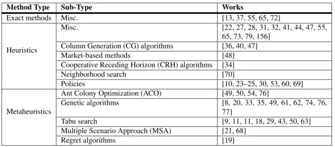
Table 3.3: Common solution methods for routing problems.
Method Type Sub-Type Works
Exact methods Misc. [13, 37, 55, 65, 72]
Heuristics
Misc. [22, 27, 28, 31, 32, 41, 44, 47, 55, 65, 73, 79, 156]
Column Generation (CG) algorithms [36, 40, 47] Market-based methods [48] Cooperative Receding Horizon (CRH) algorithms [34] Neighborhood search [70]
Policies [10, 23–25, 30, 53, 60, 69]
Metaheuristics
Ant Colony Optimization (ACO) [49, 50, 54, 76]
Genetic algorithms [8, 20, 33, 35, 49, 61, 62, 74, 76, 77]
Tabu search [9, 11, 11, 18, 29, 43, 50, 63] Multiple Scenario Approach (MSA) [21, 68]
Regret algorithms [19]
DMOMCTP is at least NP-hard (reduces to the TSP) and because this work approaches the problem from an a posteriori multiobjective perspective exact methods are assumed to be ineffective in realistic problem sizes and focus is instead placed on approximation methods.
3.3.2 Heuristics.
First, note “that no agreed definitions of heuristics and metaheuristics exist in literature, some use heuristics and metaheuristics interchangeably” [158]. For this work a slightly different but useful definition of both heuristic and metaheuristic are used which define them based on the type of information they rely upon. Specifically this work defines heuristics as problem domain specific approximation methods that require more than a black-box model to operate. This is in contrast with metaheuristics which only require a black box model to operate (but many real applications use problem-specific heuristics when creating tailored version for use). Put another way, heuristics attempt to exploit features of the problem to find good, but not optimal solutions.
Heuristics work well for single objective problems due to the relative ease in which an algorithm designer can craft such heuristics. For multiobjective problems, such heuristics may function as intended for a single objective but can have unintended side-effects
with respect to the other objectives. For example, we may use a TSP heuristic for the DMOMCTP to decrease f1(R) but this likely worsens f2(R). Similarly, we may use potential
field control methods to guide the vehicles among the nodes to avoid (O) and those to cover (W) but the algorithm may get stuck in a local optima.
Works of note utilizing heuristics include Bowerman, et al. [27] who used problem decomposition and heuristics to solve a multiobjective version of the USBRP.
3.3.2.1 Extracting Most Likely State.
One candidate solution method involves extracting the most likely state from the agent’s state model (e.g.˙probability distribution, etc.). As Russell and Norvig state, this works well “when uncertainty is small” [135]. In problems where the state transitions are uncertain but its state is fully observable the problem can be modeled as a Markov decision process (MDP). MDPs are then solved resulting in a policy, providing the optimal action given any state. When the problem is partially observable - as in the DMOMCTP - the problem can be modeled as a partially observable Markov decision process (POMDP). The solution to which is also a policy, however it is not defined with respect to the state, but the agent’s belief state. In practice POMDP methods are computationally intractable [103, 123]. Approximation methods have been presented to address this issue with promising results such as point-based value iteration [127]. Other methods include using Exponential family Principal Components Analysis (EPCA) to reduce the high-dimensional belief spaces [134].
This method may not be particularly useful for the DMOMCTP because the unknown information (what nodes will exist in the future and when they will be revealed) is not correlated to the agent’s actions, only its current time.
3.3.2.2 Robust Control.
An alternative is robust control methods which assumes a bounded amount of uncertainty and do not assign probabilities to values within that interval. Robust solutions
work regardless of the realized value as long as it exists within the assumed bounds [135]. Such methods accept uncertainty and instead formulate solutions that can still succeed given the parameters.
Works that use this method for vehicle routing include [144] which looks at the CVRP with dynamic demand from known customers (i.e. a priori). The authors refer to this problem and approach combination as the Robust Vehicle Routing Problem (RVRP). Arguably, methods such as sample-scenario as used in [68] could be described as robust control algorithms with soft bounds. In essence they reintroduce probabilities and relax the constraints, in an attempt to choose the most robust solution.
3.3.2.3 Potential Field Control.
Potential field control is a solution that lends itself to real-time control due to its low computational cost [135]. This method generates motion directly from attractive and repellent forces that pull and push the agent respectively. Assigning an attractive force to the goal position and repellent forces to the obstacles can then be used by a hill-climbing solver (or some other local search method) to move the agent. While this method is efficient it suffers from local minima (endemic to all such algorithms) that can trap the agent [111, 158].
Works utilizing this method include [142] which is the problem of collection data from a sparse sensor network. The sensors are given weights with respect to their urgency defined as the amount of data they have that needs to be collected. Other vehicles in the swarm are then given repulsive fields. Similarly, [128] utilizes potential fields to guide Autonomous Underwater Vehicle (AUV) used to create a mobile sensor network. Mei, et al. [108] combined ACO with potential fields to find efficient paths globally and locally respectively. Specifically, the local path planning element repairs the path provided by ACO when obstacles are encountered in unknown and/or dynamic environments. Li and Cassandras [99] present a receding horizon method which utilizes potential fields in a
problem domain that appears to be a variant of the OP (profits assigned to customers with deadlines).
3.3.2.4 Reactive Control.
Reactive control is a method offering low computational costs by reacting to stimuli in a deterministic fashion [135]. For example, if our agent reaches an obstacle, a reactive control rule may direct it to backtrack and alter its original path by a set amount (e.g. backup 1 meter and turn 15◦). The problem with such approaches is that the behavior can be difficult to predict in real environments. Such interplay is referred to as emergent behavior [135].
This type of control is arguably a more generalized type of policy as common in solving the DTRP (see Table 3.2 for examples). Alternatively it can be seen as repair operators common to many techniques. For example insertion heuristics in dynamic problems are a reactive method to fix the previous (and now infeasible) solution [154].
3.3.2.5 Reinforcement Learning.
Reinforcement learning is a method which produces a policy via search process. In reinforcement learning, a policy is essentially a deterministic state-to-action lookup. This method requires an accurate model of the domain, a feedback mechanism and a learning period that may be supervised (provided example input-output pairs). One difficulty with this approach is that the agent must tease out which actions were responsible for the reward or penalty which can be difficult in complex problems and/or those with long time frames. Works utilizing these methods include [117] which applied Q-learning to a problem formulation similar to the DARP. However their formulation used a weighted combination function of customer waiting time and traveling time to form a single objective. It also features vehicles with infinite capacity and, customer locations and reveal times that are not uniform (as in the DTRP). Secomandi [137] utilizes Neuro-Dynamic Programming (NDP) (aka reinforcement learning) to the VRP with dynamic demands for known customers.
Meignan, et al. [109] present a coalition based metaheuristic that has a reinforcement learning component applied to the VRP.
3.3.3 Metaheuristics.
Metaheuristics solve optimization problems as if they were black boxes with simple decisions and an output. This group includes many popular algorithms including Tabu-search, Simulated Annealing, Hill climbing, Ant Colony Optimization (ACO) and Gradient-based methods. Yang characterizes metaheuristics as:
Most metaheuristics algorithms are nature-inspired . . . Two major components of any metaheuristic algorithms are: selection of the best solutions and randomization. The selection of the best ensures that the solutions will converge to the optimality, while the randomization avoids the solutions being trapped at local minima and, at the same time, increase the diversity of the solutions. The good combination of these two components will usually ensure that the global optimality is achievable. [158]
Although metaheuristics are problem domain agnostic, many applications of them include domain-specific heuristics, operators, data types, etc. to improve their performance. This fact blurs the line between heuristics and metaheuristics, but makes their application to problems such as the DMOMCTP easier up front (i.e. specializing a general algorithm is arguably easier than generalizing a specific algorithm).
Metaheristics have been studied extensively in the routing literature, especially in multiobjective formulations due to the difficulty in designing heuristic or exact algorithms. Works using metaheuristics that are similar to the DMOMCTP include Doerner, et al. [49]. That paper compared Parallel Ant Colony Optimization (PACO), Vector Evaluated Genetic Algorithm (VEGA) [136] and Multi-Objective Genetic Algorithm (MOGA) [58] in solving a multiobjective VRP problem with a covering objective for mobile medical facilities.
This study focuses on metaheuristics due to their ease of application to new problems -especially multiobjective problems - and their performance with respect to those problems.
3.4 Summary
MOPs differ from single objective problems in that their solution’s utility is a vector. This can be handled using a priori or a posteriori methods but both require a human DM to define their preferences. This process can be difficult and is an active area of research. Since MOP solvers produce sets of solutions, the quality of those sets must be measured which can be difficult. Previous works have produced a number of metrics including hypervolume, generalized spread and generational distance. Number of constraint violations is a measure not confined to MOPs, but for problems like the DMOMCTP are important to consider because finding feasible solutions can be difficult.
The DMOMCTP enjoys a sizable amount of related works, employing a variety of methods for single and multiobjective, static and online, simple and complex routing problems. Not only are routing problems difficult (NP-complete) but the most effective methods can change rather drastically between problem domains. This leaves us with only hints as to what will work well for the DMOMCTP which forms the impetus behind this work.