Multi-parametric mixed integer linear programming under global uncertainty

Contents lists available at ScienceDirect

Computers

and

Chemical

Engineering

journal homepage: www.elsevier.com/locate/compchemeng

Multi-parametric

mixed

integer

linear

programming

under

global

uncertainty

Vassilis

M.

Charitopoulos,

Lazaros

G.

Papageorgiou

,

Vivek

Dua

∗

DepartmentofChemicalEngineering,CentreforProcessSystemsEngineering,UniversityCollegeLondon,TorringtonPlace,LondonWC1E7JE,United Kingdom

a

r

t

i

c

l

e

i

n

f

o

Articlehistory: Received15September2017 Revised12April2018 Accepted13April2018 Availableonlinexxx Keywords:

Optimisationunderuncertainty Multi-parametricprogramming Mixedintegerlinearprogramming Cylindricalalgebraicdecomposition Grobnerbases

Processscheduling

a

b

s

t

r

a

c

t

Majorapplicationareasoftheprocesssystemsengineering,suchashybridcontrol,schedulingand syn-thesiscanbeformulatedasmixedintegerlinearprogramming(MILP)problemsand arenaturally sus-ceptibletouncertainty.Multi-parametricprogrammingtheoryformsanactivefieldofresearchandhas proventoprovideinvaluabletoolsfordecisionmakingunderuncertainty.Whileuncertaintyinthe right-handside(RHS)andintheobjectivefunction’scoefficients(OFC)have beenthoroughlystudiedinthe literature,thecase ofleft-hand side(LHS)uncertainty hasattractedsignificantlyless attention mainly becauseofthe computationalimplicationsthat ariseinsuchaproblem.Inthe presentwork,we pro-poseanovelalgorithmfortheanalyticalsolution ofmulti-parametricMILP(mp-MILP)problemsunder globaluncertainty,i.e.RHS,OFCandLHS.Theexactexplicitsolutionsandthecorrespondingregionsof theparametricspacearecomputedwhileanumberofcasestudiesillustratesthemeritsoftheproposed algorithm.

© 2018TheAuthors.PublishedbyElsevierLtd. ThisisanopenaccessarticleundertheCCBYlicense.(http://creativecommons.org/licenses/by/4.0/)

1. Introduction

Mathematical modelling is a non trivial task that requires deep and thorough understanding of the principles and phenomena in- volved in the problem under study. Inevitably, mathematical mod- elling relies on a number of assumptions and simplifications due to lack of exact knowledge about the system under examination, thus rendering any solution liable to uncertainty. The classification of uncertainty in optimisation problems is a challenging task but broadly one could classify the uncertainty as model intrinsic and extrinsic. Model intrinsic uncertainty refers to a number of param- eters that the modeller does not have explicit knowledge of, e.g. kinetic constants, stoichiometric coefficients, equipment efficiency etc. For this kind of uncertainty, the value used in the models is experimentally calculated or provided by the manufacturer of the equipment; even in that case, these values cannot be known ex- actly and a number of assumptions is usually employed. Note that this kind of uncertainty, appears most of the times on the left- hand side (LHS) of the constraints. On the other hand, model ex- trinsic uncertainty refers to data that affect the model due to fac- tors which cannot be controlled at a level of model abstraction. Ex- amples of model extrinsic uncertainty can be regarded as, the cost

∗ _{Correspondingauthor.}

E-mailaddress:[email protected](V.Dua).

of raw material, emissions restriction policies, product demand for subsequent planning periods etc. This kind of uncertainty is more likely to appear on the right-hand side (RHS) of the constraints and in the objective function’s coefficients (OFC). Consideration of un- certainty in process systems engineering is of great importance as it can endanger the optimality or even the feasibility of a solu- tion that was computed in a deterministic way ( Apapand Gross-mann,2017;Sahinidis,2004). In an effort to avoid such occasions, a number of mathematical formulations and solution techniques have been proposed in the literature with the goal to create mod- els which are robust towards uncertainty. Stochastic programming

( Apap andGrossmann,2017; Bertsimas andSim,2004; Birgeand

Louveaux,2011) relies on the availability of historical data which can provide statistical information about the behaviour of uncer- tain parameters. In stochastic programming, the unknown parame- ters are assumed to follow a discrete probability distribution and the decision variables are classified into two groups: “here and now” and “wait and see”. Depending on the instances that the un- certainty is expected to be revealed, the mathematical program is referred to as “two-stage” or “multi-stage” with the objective to minimise the cost of the initial actions. Robust optimisation (RO), assumes that all constraints of the optimisation should never be violated and aims to provide a solution that is feasible regardless of the extent of the actual uncertainty. Because of that, RO is of-

https://doi.org/10.1016/j.compchemeng.2018.04.015

0098-1354/© 2018 The Authors. Published by Elsevier Ltd. This is an open access article under the CC BY license. (http://creativecommons.org/licenses/by/4.0/)

Table1

Summaryofdevelopmentsinmulti-parametricprogrammingtheory.

Multi-parametric SaatyandGass(1954),YufandZeleny(1976),Schechter(1987) Linearprogramming

(mp-LP)

Gal(1995),Borrellietal.(2003),Filippi(2004),Hladík(2010),Charitopoulosetal.(2017a) Multi-parametric(mixed

integer)

Duaetal.(2002),Bemporadetal.(2002),TøNdeletal.(2003) Quadraticprogramming

(mp-(MI)QP)

Spjøtvoldetal.(2006),Guptaetal.(2011),OberdieckandPistikopoulos(2015) Multi-parametricmixed

integer

GeoffrionandNauss(1977),Jenkins(1990),AcevedoandPistikopoulos(1999) Linearprogramming

(mp-MILP)

DuaandPistikopoulos(2000),Faíscaetal.(2009) Multi-parametric(mixed

integer)

DuaandPistikopoulos(1998,1999) Nonlinearprogramming

(mp-(MI)NLP)

AcevedoandSalgueiro(2003),Pistikopoulosetal.(2007),Fotiouetal.(2006),CharitopoulosandDua(2016), Charitopoulosetal.(2017b)

Multi-parametric Fiacco(1990),Duaetal.(2004) Globaloptimisation

(mp-GO)

Wittmann-HohlbeinandPistikopoulos(2012a),Oberdiecketal.(2014)

ten conceived as conservative or worst-case oriented ( Ben-Taland Nemirovski,2002).

For the study of the effect of uncertain parameters on the op- timal solution, the two main methodologies reported in the open literature are: sensitivity analysis and (multi-)parametric program- ming. The former provides information about the effect of un- certainty around the neighbourhood of the nominal value while the latter characterises explicitly its effect on the optimal solution throughout the entire range of parametric variability. Next, we re- view the developments in multi-parametric programming theory in order to familiarise the reader with the topic of this article.

1.1.Literaturereview

Multi-parametric programming (mp-P) is an optimisation based technique which systematically studies the effect of uncertain pa- rameters on the optimal solution of mathematical programming problems. Through multi-parametric programming, one aims to compute offline, the explicit optimal solution to a mathematical program which consists of two parts:

• The optimisers and the optimal objective value as functions of the uncertain parameters, i.e. x(

θ

) and z(

θ

), respectively. • The regions of the parametric space where each explicit solu-

tion remains optimal. These regions are also known and will be referred to for the rest of the article as critical regions (CRs). The distinct feature of mp-P is the fact that, under the presence of uncertainty, the need for constant re-optimisation is replaced by efficient function evaluations that can be performed online when- ever the uncertainty is realised. For this reason, mp-P has attracted the interest of many researchers and the main milestones in the history of mp-P are summarised in Table1.

Gass and Saaty ( 1954,1955a,1955b) shortly after the invention of the simplex algorithm studied the parametric analysis of the optimal solution for Linear Programming (LP) problems when un- certain cost coefficients are considered in the objective functions. However, the first systematic framework for (multi-)parametric lin- ear programming (mp-LPs) problems was proposed by Gal and Ne- doma ( 1972,1975) who studied the solution of mp-LPs with per- turbation on the RHS of the constraints and/or the OFC, i.e. RIM- mp-LP. For the case of mp-LPs the majority of the algorithms employ the optimal basis invariancy to create the correspond- ing CRs and compute the explicit optimisers. On the contrary, Borrellietal.(2003) proposed an algorithm for the solution of mp- LPs based on the direct exploration of the parametric space study- ing the underlying geometry of the problem. Another algorithm for mp-LP problems was proposed by Jones andMorrari (2006) who

revisited the classic mp-LP as linear complementary problems and employed lexicographic perturbation to efficiently deal with de- generacy in mp-LPs. Note that the aforementioned algorithm can handle RIM-mp-LP problems as well as multi-parametric quadratic programming (mp-QP) problems.

Multi-parametric mixed integer linear programming (mp-MILP) problems, have been studied by AcevedoandPistikopoulos(1999), DuaandPistikopoulos(2000), LiandIerapetritou(2007a) to name a few. For the solution of mp-MILPs the decomposition approach of DuaandPistikopoulos(2000) has proven to be computationally advantageous compared to the rest. It involves an iterative scheme between the solution of a master MIP problem and slave mp-LPs until the master MIP is infeasible. During this procedure, integer and parametric cuts are employed to prevent investigation of pre- viously explored solutions.

Multi-parametric (mixed integer) quadratic programming (mp- (MI)QP) problems form another important class of mp-P prob- lems due to their application in optimal control schemes. The first algorithm for mp-QPs was devised by Dua(2000) where the Karush–Kuhn–Tucker (KKT) conditions of optimality were solved explicitly and was later on applied in the seminal work of Bemporad etal. (2002) leading to the concept of explicit model predictive control, while in Duaetal.(2002) the mp-MIQP prob- lems were treated.

The global optimisation of non-convex mp-NLPs and mp-MILPs with RHS uncertainty was initially discussed by Dua et al. (2004) and the authors proposed four different para- metric convex overestimators along with a B&B algorithm. Note that Fiacco (1990) had proposed a solution technique for global optimisation for the case of non convex multi-parametric sepa- rable NLPs restricted to a convex set. Another algorithm for the global optimisation of mp-MILPs for RIM problems was proposed by Faísca et al. (2009). The authors follow the decomposition scheme as in Pertsinidis et al. (1998) and Dua and Pistikopou-los(2000) where the integer vector is fixed by the solution of a master MINLP to global optimality and then is fixed resulting in a slave mp-LP. Despite the merits of the aforementioned algorithm, because of the non-convex nature of the problem, the comparison procedure of overlapping CRs is not always computationally possi- ble and thus the authors for these cases store the corresponding solutions in a parametric envelope and the best one is chosen online through function evaluation.

Wittmann-HohlbeinandPistikopoulos(2012b) proposed a com-

putationally efficient two stage method for the approximate solu- tion of mp-MILPs under global uncertainty. In order to handle LHS uncertainty, the authors employ worst-case oriented RO and thus render the initial problem partially immune to uncertainty. The

partially immune problem is practically an RIM-mp-MILP problem which can be solved by existing algorithms. Note that although RO can handle efficiently LHS uncertainty, the resulting solution can be overly conservative or even unbounded for some instances. As far as the explicit solutions are considered, again no compari- son procedure is followed and the determination of the best so- lution is done via online evaluation. Later on, the same authors ( Wittmann-Hohlbein and Pistikopoulos, 2012a) studied mp-MILP problems with only LHS uncertainty. When LHS is introduced to the problem, bilinear terms arise either in the form of

θ

_·x or

θ

·y rendering the problem a non-convex mp-MINLP. The proposed spatial B&B scheme from this work encompasses the construction of suitable McCormick envelopes that transform the LHS uncer- tainty to RHS and branching schemes on the optimisation variables and/or uncertain parameters. Computational studies showed that the algorithm can be computationally onerous as it results in a large number of CRs and also the quality of the solution is highly dependent on the branching scheme selected. Nevertheless, this work underlines the complexity of the resulting mp-P when LHS is considered. Global uncertainty in general mp-MILPs was also stud- ied by LiandIerapetritou (2007a) and the authors employed the optimality conditions of LPs for the definition of explicit solutions by retrieving the corresponding optimal bases. When LHS uncer- tainty was also considered, projection schemes were employed and approximations of the non-convex CRs were computed. Finally, a solution algorithm for the single parametric case of LHS in p-LPs was devised by KhalilpourandKarimi(2014) that included inver- sion techniques of perturbed matrices.

1.2. Problemstatement

The aim of this article is to provide a solution algorithm for the most general case of mp-MILPs, i.e. the case where uncertain pa- rameters appear simultaneously on the RHS, OFC and LHS (global uncertainty). mp−MILPGlobal =

⎧

⎪

⎪

⎪

⎨

⎪

⎪

⎪

⎩

z

(

θ

)

= min x,y c T

₍

_θ

₎

_{x + d}T

₍

_θ

₎

_y subjectto: A

(

θ

)

x + W

(

θ

)

y ≤b

(

θ

)

(

θ

)

x +

(

θ

)

y =

γ

(

θ

)

x ∈X⊆Rn x, _y ∈

{

₀,₁

}

n y

θ

∈

⊆Rθ (1)

Problem (1), is a multi-parametric programming problem with non-convex parametric objective function and a non-convex fea- sible set. The non-convexity of the parametric objective function arises from the bilinear terms in the form of either cT (

θ

) ·x or

dT (

θ

) ·y. The parametric feasible set of (1) is also non-convex be- cause of the presence of bilinear terms between the optimisation variables, i.e. x and the uncertain entries of the technology matrix, i.e. A(

θ

). As already stated in the previous section of the article, the aforementioned problem remains as one of the biggest challenges because of its computational complexity. The challenges involved in the solution of problem (1) are:

• The computation of the explicit optimisers, i.e. x(

θ

), and the CRs where each explicit solution is optimal.

• Because of the non-convex nature of the problem it is likely that a number of CRs overlap in the same region of the para- metric space. In order to provide at the end one explicit solu- tion per CR, one needs to follow a comparison procedure which in the state of the art requires solving a number of MINLPs to global optimality.

Many problems in PSE can be formulated as MILPs and thus providing a solution technique for mp-MILPs under global uncer- tainty can significantly enhance the applied value of such solu- tions. Acevedo and Pistikopoulos (1997) studied the problem of plant synthesis under demand uncertainty while uncertainty in

Table2

mp-MILPalgorithms.

Algorithm Uncertaintyclass Explicitsolutions perCR RHS OFC LHS AcevedoandPistikopoulos(1999) 1 DuaandPistikopoulos(2000) 1 LiandIerapetritou(2007a) ₁

Faíscaetal.(2009) 2

Wittmann-Hohlbeinand Pistikopoulos(2012a)

1

Oberdiecketal.(2014) 1.3

process planning has also been formulated as a parametric prob- lem ( Pistikopoulos andDua, 1998). Process scheduling forms an- other important class of problems that has been studied through parametric programming. Ryuetal.(2007) studied the scheduling of zero-wait batch processes and they considered variable process- ing times after the employment of linearisation techniques. Jiaand Ierapetritou (2006) proposed a framework for RHS uncertainty in scheduling problems that leads to the solution of an mp-MILP problem. LiandIerapetritou(2007b) provided a generalised frame- work for process scheduling under uncertainty where depending on the topology of the uncertainty (RHS, LHS, OFC) different mixed integer mp-P problems had to be solved.

Despite the considerable attention that mp-P has drawn from the research community ( CharitopoulosandDua,2017; Pistikopou-losetal.,2012) the solution of mp-MILPs under global uncertainty remains one of the least studied problem due to the computational complexity involved. In Table 2 an updated summary of the pro- posed algorithms for mp-MILPs is presented along with the classes of uncertainty that can be handled. In the third column of Table2, the average number of explicit solution per CR is given based on computational studies reported in corresponding papers. To the best of our knowledge, no previous research work has been pro- posed for the exact solution of problem (1) without the employ- ment of projection or discretisation techniques or through a hybrid optimisation scheme. In the present work, we propose a novel al- gorithm for the exact solution of general mp-MILPs under global uncertainty based on the principles of symbolic manipulation and semi-algebraic geometry. A significant feature of the proposed al- gorithm lies in the exact computation of non-convex CRs where only one globally optimal explicit solution is stored and no need for online comparison is needed.

The remainder of the article is organised as follows: in Section2, we introduce the reader to the main concepts that form the basis for the present work. Then we illustrate the main steps of the proposed algorithm while the nature of the optimal explicit solution and the CRs is discussed. To illustrate the solution proce- dure, in Section3, a number of examples are solved. Process syn- thesis and scheduling case studies underline the potential practi- cal value of the proposed algorithm. A short discussion about the computational issues and non-convexity of the problem follows in Section 4. Finally, concluding remarks and future research direc- tions are outlined in Section5.

2. Methodology

2.1. Gr¨o bnerbasestheory

The key idea of the proposed algorithm is as follows. Instead of approaching the solution of the mp-P problem numerically we exploit concepts from computer algebra. Upon inspection, problem (1) involves bilinear terms of optimisation variables with uncertain parameters and within the context of computer algebra this can

be viewed as a “power-product”. Based on this inspection, Gr ¨o bner bases theory can be employed for the solution of square system of equations that is derived by the 1st order KKT conditions of prob- lem (1). Before we proceed further it is important to provide some formal definitions that are crucial in Gr ¨o bner bases theory.

Let k be any field and let k[ x] =k[ x1,...,xt ] be the ring

of polynomials in t indeterminates. Any polynomial can be de- scribed as a sum of terms of the form:

α

xβ1₁ ...xβt

t with

α

∈k and

β

i ∈N, i= 1 ,...,t and the term xβ11 ...xtβt is called power-product.

Definition1. Gro¨bner basis ( Buchberger,2006)

A set of non-zero polynomials G₌

{

g1,...,gt

}

contained in an ideal I, is called a Gro¨bner basis for I if and only if for all f∈I such that f=0, there exists i∈

{

1 ,...,t

}

such that lp( g_i ) divides lp( f), where lp( _·) stands for the leading power-product of a polynomial function.

In the definition given, an ideal is a set of polynomials of the form

[

i= 1 ] tu_i g_i with g_i in G and arbitrary polynomials u_i . The existence of such ideal is guaranteed by the Hilbert Basis theorem ( BuchbergerandWinkler,1998), which also guarantees the termi- nation of algorithms that are used for the computation of Gro¨bner

bases.

Roughly speaking, within Gro¨bner bases theory a set of polyno- mial V is transformed into an other set of polynomials G which is equivalent to the former but has certain favourable computational properties. At the core of Gro¨bner bases theory the Buchberger al- gorithm is found ( Buchberger, 2006) which is employed for the computation of the Gro¨bner basis of a specific set of polynomi- als. Buchberger introduced within the algorithm the concept of S- polynomials as well as provided a theorem for the proposed algo- rithm which for the sake of space are not discussed in the present article; however, the interested reader can refer to the book of BuchbergerandWinkler(1998) for further exposition on the sub- ject. Apart from Buchberger’s algorithm for the computation of

Gro¨bner bases, Faug e`re devised two algorithms, F4 ( Faugere,1999) and F5 ( Faugere,1998) which compared to Buchberger’s algorithm are computationally more efficient. F4 is based on linear alge- bra principles where successive truncated Gro¨bner bases are cre- ated and reductions of the polynomials are performed in parallel; within the algorithmic routine a symbolic preprocessing step is in- cluded as well as the author adopted the Buchberger’s criteria for the selection of the critical pairs of power-products.

Note, that Mathematica 10, the computer algebra system (CAS) where the proposed algorithm is implemented uses an optimised version of the Buchberger’s algorithm.

2.2.Globaluncertaintyingeneralmp-MILPs

Let us consider again the mp-MILPs under global uncertainty. Without loss of generality consider the case where the equality constraints are replaced by opposing inequality constraints thus leading to the form of problem ( Pmaster ).

(

Pmaster

)

=

⎧

⎪

⎨

⎪

⎩

z

(

θ

)

= min x,y c T

₍

_θ

₎

_{x + d}T

₍

_θ

₎

_y subjectto: A

(

θ

)

x + W

(

θ

)

y ≤b

(

θ

)

x ∈ X ⊆Rn x, _y ∈

{

₀,₁

}

n y

θ

∈

⊆Rθ (2)

Problem ( P_master ) is an mp-MILP that involves uncertain param- eters on the RHS, LHS and OFC. The key idea is to treat both the uncertain parameters and the binary variables as symbols and thus reduce ( P_master ) to an mp-LP under global uncertainty at the first stage. Another idea would be to follow a decomposition scheme similar to DuaandPistikopoulos(2000) where the decision maker would iterate between the a Master MILP and slave symbolic mp- LPs; however we do not explore this option in the present work

as results from the case studies indicate the dimensionality of the binary variables do not affect significantly the computational com- plexity of the proposed scheme. Note that idea for the relaxation of the binary variables as uncertain parameters has been used in some of our previous works ( CharitopoulosandDua,2016; Chari-topoulosetal.,2017b;Dua,2015;GueddarandDua,2012). Treating the binary variables as uncertain parameters between their respec- tive lower and upper bound results in a relaxed mp-MILP (R-mp- MILP) which can be solved analytically.

(

R−mpMILP

)

⎧

⎪

⎪

⎪

⎨

⎪

⎪

⎪

⎩

z

(

θ)

=min x,y c T

₍

_θ)

_x+dT

₍

_θ)

_y subject to : A

(

θ)

x+W

(

θ)

y≤b

(

θ)

x∈X

{

x∈Rnx

|

_xmin k ≤xk ≤xmax k ,k=1 ,...,nx

}

y∈[0 ,1] n y

θ

∈

{

θ

∈Rn θ

|

θ

_lmin _≤

θ

_l≤

θ

max l ,l=1 ,...,nθ

}

(3)

The R-mp-MILP is an augmented mp-P where apart from the uncertain parameters we consider the relaxed binary variables. For- mulating the first order KKT conditions for the R-mp-MILP leads to the system of Eq.(4).

(

P

)

⎧

⎨

⎩

∇

xL

(

x , y ,

θ

)

= 0

λ

j

(

y ,

θ

)(

[ k= 1]nx aj,k

(

θ

)

xk + [ k= 1]ny wj,k

(

θ

)

yk −bj

(

θ

))

= 0,

∀

j = 1,...,m (4) where L

(

x,y,

θ

,

λ

)

=cT

(

θ

)

x+dT

(

θ

)

y+

λ

T

₍

m j=1 n x k=1aj,k

(

θ

)

xk + m j=1 n y

k=1wj,k

(

θ

)

yk −bj

(

θ

))

is the Lagrangian function of the R- mp-MILP problem. Solving ( P) analytically results in the explicit parametric expressions of the optimisation variables, i.e. x( y,

θ

) and the Lagrange multipliers, i.e.

λ

( y,

θ

) which will be used in the next step to evaluate the optimality and feasibility conditions, i.e. the non-negativity of the Lagrange multipliers and the satisfaction of the inactive constraints. The set of solutions computed at this step are called “candidate solutions”. Candidate solutions, include so- lutions that can be locally or globally optimal or infeasible due to constraint violation or integrality conditions. In the evaluation of the candidate solutions the first step is to consider the non- negativity of the Lagrange multipliers which would lead to the re- jection of infeasible solutions. Note that by doing so, we avoid to visit every possible integer node and thus reduce the computa- tional burden. As next step, we impose the integrality conditions on the binary variables, i.e. y∈[0 ,1] n y→_y∈

{

₀ ,₁

}

n y_{; as a result}

now the Lagrange multipliers and the vector of optimisation vari- ables are functions of the uncertain parameters. i.e. x(

θ

),

λ

(

θ

) and the feasibility and optimality qualification is performed so as to compute the final “integer feasible solutions”. Note that at the end of this step, for the “integer feasible solutions” the corresponding CRs are given by the inequality constraints (5) and (6).

λ

j

(

θ

)

≥0, j = 1,...,m ⇒ optimalityconditions (5) g _j

(

θ

)

≤0, j = 1,...,m ⇒ feasibilityconditions (6) where g_j (

θ

) stands for the vector of inequality constraints of prob- lem (R-mpMILP) that is now explicit only in

θ

. If the solution under evaluation is feasible, then the inequality constraints provide a set of parametric inequalities that form the CR of the integer feasible solution.

Remark1. When global uncertainty is considered in mp-MILPs the explicit optimisers and the optimal objective value, i.e. x(

θ

) and

z(

θ

), are fractional polynomial functions of the uncertain parame- ters continuous within their respective CR but not necessarily con- tinuous in the entire parametric space. The corresponding CRs are in general non-convex and possibly discontinuous ( Charitopoulos etal.,2017a;Wittmann-HohlbeinandPistikopoulos,2012a).

Table3

PossibleoutcomesinthedefinitionofCRINT.

Case1

CR1⊆CR2whichmeansthatallconstraintsofCR2areredundant andCRINT =CR1

Case2 CR1⊇CR2whichmeansthatallconstraintsofCR1areredundant andCRINT =CR2

Case3 TheCRINTisdefinedbyasetofactiveconstraintsfromboth

CR1andCR2asboth

CRshavesomenon-redundantconstraints

Because of the combinatorial nature of the problem, it is com- mon issue mp-P that some CRs may co-exist in the same space and thus requiring some dominance criterion so as to decide upon the dominant CR in the common parametric space; in this work we follow the same procedure for the comparison and dominance of overlapping CRs from our latest work ( CharitopoulosandDua, 2016;Charitopoulosetal.,2017a).

2.3. Cylindricalalgebraicdecompositionandcomparisonof

overlappingCRs

Defining redundant constraints and computing the new CRs within the comparison procedure is a non-trivial task, especially for non-convex problems. A comparison procedure for explicit solutions valid in the same parametric space can be found in Acevedo and Pistikopoulos (1997). This procedure is applicable only for the case of convex CRs, i.e. when the CRs are defined as a set of linear inequality constraints. In general, while solving a mp- MILP problem under global uncertainty it can happen that two dif- ferent parametric solutions, i.e. z1(

θ

) and z2(

θ

) to be feasible in the

same parametric space. The comparison procedure aims to identify the regions where:

z1

(

θ

)

−z2

(

θ

)

≤0 (7)

and

z2

(

θ

)

−z1

(

θ

)

≤0 (8)

given that z1(

θ

) is valid in CR1 and z2(

θ

) is valid in CR2. The first

step is to compute CRINT=CR1∩CR2.

2.3.1. ComputationofCRINTandredundantconstraints.

Excluding the case that CR_INT =∅ there are three possible out- comes in the definition of the CR_INT which are described in Table3

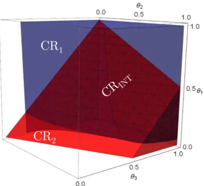
In Fig. 1 the different cases for the definition of the CR_INT can be envisaged.

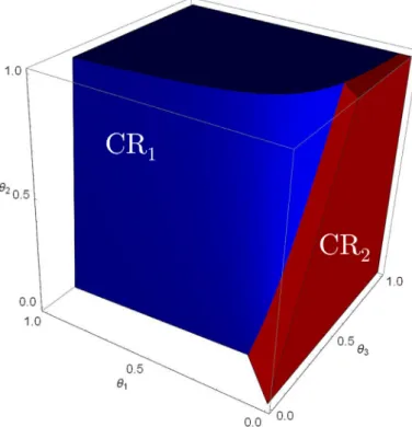
For illustration purposes assume that the following two ran- domly generated CRs, given by Eqs.(9) and (10), are under exam- ination. We have chosen to illustrate a case that one of the CRs is convex the other one non-convex and their overlap ( CR_INT ) is non- convex as well, in order to underline the salient feature of the pro- posed algorithm, i.e. computing exact non-convex CRs. Graphically, in the parametric space CR1and CR2 are presented in Fig.2.

CR1 =

0 ≤

θ

1,

θ

2,

θ

3 ≤1

θ

1 −θ_θ2₁+ 25

θ

3 ≥25 (9) CR2 =

0 ≤

θ

1,

θ

2,

θ

3 ≤1

θ

3 −

θ

1 ≥0.5

θ

2 (10)

CR1 is non-convex while CR2 is convex as polyhedral and thus

previously proposed methods for computing their potential over- lap are not applicable without some kind of convex approxima- tion. Moreover, identifying redundant constraints and computing the “dominant” CRs infers a problem of solving inequalities which are quantified by logical operators (

∃

,

∀

, ∧, ¬ etc.). It can be un- derstood that posing the problem of computing the overlap be- tween two CRs is equivalent to posing the question “is there any

range of uncertain parameters for which any inequalities that form the CRs are simultaneously satisfied?”. This question can be in turn postulated as the following quantified mathematical formula:

{∃

θ|

CR_{i ∧}CR_{j ,} for i₌ j

}

where _∧ stands for the “logical and” op- erator. One of the most widely known and used algorithms for the solution of quantified systems of inequalities is the Cylin- drical Algebraic Decomposition (CAD) algorithm ( Jirstrand, 1995; Strzebo´nski,2000). In brief, one by computing the CAD of a sys- tem of inequalities after a number of projection in the decision space (the parametric space in the case of interest for the present work) partitions the space into a sets of, typically non-convex, re- gions where each inequality retains a constant sign. By doing so, one can evaluate whether a set of inequalities is satisfied within certain regions and at the end compute the final solution to the system of inequalities (in our case, a CR itself, an overlap among different CRs or the region of the parametric space where an ex- plicit solution dominates another). For a detailed exposition on the subject of cylindrical algebraic decomposition the interested reader is referred to the tutorial article of Jirstrand(1995).

As mentioned above, in the present work Mathematica was em- ployed for the analytic solution of the mp-MILP under global un- certainty. Specifically, for the comparison procedure the command “Reduce” was employed which involves an implementation of the CAD algorithm. “Reduce” is a command in Mathematica that qual- ifies sets of conditional arguments within a given set of parame- ters and computes a new set within which these conditional state- ments are satisfied. A detailed exposition on the specifics of the function can be found in Strzebo´nski (2000) where the author details the different strategies employed internally in Mathemat- ica. For example in the definition of the intersection of two CRs ( CR_INT ), “Reduce” identifies the redundant constraints of both CRs and computes the region of parametric space where both CRs ex- ists; for the case that the CRs do not overlap the output of “Re- duce” is a “False” statement equivalent to the argument CR_INT =∅. Defining the CR_INT thus infers computing the CAD of the para- metric space where both CR1 and CR2 are always valid and a part

of its mathematical expression is given by Eq.(11). In Fig. 1 the meshed area of the parametric space represents the overlap of the two CRs. CRINT =

⎧

⎪

⎪

⎪

⎪

⎪

⎪

⎪

⎪

⎪

⎪

⎪

⎪

⎨

⎪

⎪

⎪

⎪

⎪

⎪

⎪

⎪

⎪

⎪

⎪

⎪

⎩

0 <

θ

1≤0 .049

0 ≤

θ

2≤

θ

1

(

20 +

θ

1

)

0 .2 −0 .04

θ

1+0.04_θθ2 1 ≤

θ

3≤1 0 .049 ≤

θ

1≤0 .099

0 ≤

θ

2≤1 0 .2 −0 .04

θ

1+0.04_θθ2 1 ≤

θ

3≤1 . . . . . . 0 .5 ≤

θ

1≤1

0 ≤

θ

2<2 −2

θ

1

θ

1+0 .5

θ

2≤

θ

3≤1 (11)

The redundant constraints from each CR can be computed as

RC_CR

i=

{

θ|

θ

∈

(

CRi ∧

(

¬CRINT

))

}

,

∀

i=1 ,2 using CAD computations.

2.3.2. ComputationofCRREST andthefinalnon-overlappingCRs.

After the definition of the CR_INT the dominance criterion can be expressed by the conditional inequality (12).

z1

(

θ

)

−z2

(

θ

)

≤0,

θ

∈ CRINT (12) As a next step, excluding the case that CR_INT =∅, the compar- ison procedure is continued and a new set of conditional state- ments is qualified, given by (12). The output of this step is used so as to define the CR_REST

i, given by (13) and (14), while the two

modified CRs after the comparison procedure no longer overlap.

CR_REST 1=

{

θ

|

θ

∈

(

CRINT ∧

(

z1

(

θ

)

≤z2

(

θ

)

)

}

(13)

Fig.1. DefinitionofCRINT.

Fig.3. Finalnon-overlappingCRsintheparametricspace.

Following the comparison procedure for the previous illustra- tive case, assume that z1

(

θ

)

−z2

(

θ

)

=−2

θ

1−19

θ

2+2

θ

3−68 . In

order to identify the dominant solution for the illustrative case the related CAD is computed in order to evaluate (12). The out- put of the “Reduce” in the present case a new set of inequalities, namely CR_Rest ; this is the fraction of CR_INT in which z1(

θ

) ≤z2(

θ

).

More specifically in the case, the explicit solution of CR1is always

dominant in the overlap of the two CRs and thus CR_REST

1≡CRINT

while CR_REST

2=∅.

After the CR_REST regions are computed the final CRs can be com- puted as follows:

CR₁f in =

{

θ

|

θ

∈

(

CR1 ∧

(

¬ CRREST 2

)

}

(15)

CR₂f in =

{

θ

|

θ

∈

(

CR2∧

(

¬ CRREST 1

)

}

(16) Finally, the two CRs that no longer overlap are presented graph- ically in Fig. 3, the mathematical expression of CR2 is given by

Eq. (17) while the mathematical expression of CR1 remains the

same as the one given by Eq.(9). Notice that z1(

θ

) is globally op-

timal in CR₁f in and z2(

θ

) is globally optimal in CR2f in .

CR₂f in=

⎧

⎪

⎪

⎪

⎪

⎪

⎪

⎪

⎪

⎪

⎪

⎪

⎪

⎪

⎨

⎪

⎪

⎪

⎪

⎪

⎪

⎪

⎪

⎪

⎪

⎪

⎪

⎪

⎩

θ

3 ≤1

⎧

⎪

⎪

⎪

⎨

⎪

⎪

⎪

⎩

θ

1 = 0

θ

2 = 0 &

θ

3 ≥0 0 ≤

θ

2≤1 &0.5

θ

2≤

θ

3

θ

1>0 &

θ

1

(

θ

1 + 20

)

<

θ

2 ≤1&

θ

1+ 0.5

θ

2 ≤

θ

3

θ

1 = 0.0498 &0 ≤

θ

2 ≤1&0.5

θ

2+ 0.0498≤

θ

3<0.198+ 0.8019

θ

2

θ

2 ≥0

⎧

⎪

⎪

⎨

⎪

⎪

⎩

0.04

θ

1+

θ

3<0.2+ 0.04_θ1θ2 &

θ

1 + 0.5

θ

2 ≤

θ

3

⎧

⎪

⎨

⎪

⎩

θ

1>0.0992&

θ

1

(

θ

1

(

θ

1 + 0.48

θ

2 −0.272

)

−0.0769

θ

2+ 0.0153

)

+ 0.003

θ

2<0

)

0<

θ

1<0.0498&

θ

2<

θ

1

(

θ

1 + 20

)

0.0498<

θ

1<0.0992&

θ

2≤1.

θ

1 = 0.0992&0.5

θ

2 + 0.0992 ≤

θ

3 &

θ

3<0.40318

θ

2+ 0.196 0<

θ

1<0.0498&

θ

2 =

θ

1

(

20+

θ

1

)

&

θ

1+ 0.5

θ

2 ≤

θ

3<1 (17)

A flowchart of the main steps for the exact solution of general mp-MILPs under global uncertainty is given in Algorithm1 while a more elaborate description is given in Algorithm S.2.

Remark 2. Note that when LHS uncertainty is considered in the coefficients of the binary variables exact linearisation techniques can be employed to transform the LHS to RHS uncertainty. More specifically, following the Glover transformation ( Glover,1975) the product between an uncertain parameter and a binary variable, for the case of non-negative uncertain parameter, can be ex- pressed with the help of an artificial variable, i.e.

θ

RHS=

θ

·y, as:

(

y−1

)

θ

up +

θ

≤

θ

RHS ≤

θ

up ,

θ

RHS ≤

θ

.

Remark 3. Note that despite the fact that in the proposed algo- rithm we refer only to binary variables the algorithm is applica- ble to integer variables too, as illustrated in a similar work by Dua(2015).

3. Casestudies

In the present section the main steps of the proposed algorithm are demonstrated on a number of illustrative examples and case studies.

3.1.Example1:mp-MILPwithLHSuncertainty

In order to illustrate to applicability of the proposed method- ology for the case of mp-MILPs we consider the following mp- MILP problem with LHS uncertainty ( Wittmann-Hohlbeinand Pis-tikopoulos,2012a). LHS−mpMILP

⎧

⎪

⎪

⎪

⎪

⎪

⎪

⎪

⎪

⎪

⎨

⎪

⎪

⎪

⎪

⎪

⎪

⎪

⎪

⎪

⎩

z

(

θ

)

= min x,y

(

−2x1 −x2 +y1 +y2

)

subjectto: x1 +

(

3+

θ

1

)

x2 + y1 ≤9

(

2+

θ

2

)

x1 + x2 −y2 ≤8 x1 −y1 +y2 ≤4 0 ≤x1 ≤4,0 ≤x2 ≤3 y1,2 ∈

{

0,1

}

, −10≤

θ

1,2 ≤10 (18)

Following the proposed algorithm, first the Lagrangian function of problem (18) is formulated as shown in Eq.(19).

L

(

x1,x2,y1,y2,

θ

1,

θ

2,

λ

1,

λ

2,

λ

3,

λ

4,

λ

5,

λ

6,

λ

7

)

= −2x1−x2+ y1+ y2+

λ

1

(

x1+

(

3+

θ

1

)

x2+ y1−9

)

+

λ

2

(

2+

θ

2

)

x1+ x2 −y2 −8

)

+

λ

3

(

x1−y1+ y2−4

)

+

λ

4

(

−x1

)

+

λ

5

(

−x2

)

+

λ

6

(

x1−4

)

+

λ

7

(

x2 −4

)

(19)

Next, the gradient of the Lagrangian is computed with respect to the optimisation variables, i.e. x1, x2 and is given in Eq.(20).

∇

x 1,x 2L = [

(

θ

2 + 2

)

λ

2 +

λ

1+

λ

3−

λ

4 +

λ

6 −2,

(

θ

1+ 3

)

λ

1

+

λ

2−

λ

5+

λ

7 −1]T (20)

Note that the components of the gradient of the Lagrangian are explicit in

θ

and

λ

and also because of the existence of uncertain parameters in the constraint matrix nonlinear products of the form

λ

·

θ

are present. After the gradient of the Lagrangian is computed, the first order KKT conditions are formulated and this results in a square system of 9 equations and 9 unknowns. More specifically,

nx equations are from the condition that the gradient of the La- grangian must be zero and ng equations are given by the strict complementary slackness conditions. Solving the KKT system, re- sults in 17 candidate solutions as shown in Table4.

It takes 0.12 s for Mathematica to compute 17 candidate so- lutions for problem (18) of which, after qualifying with the non- negativity condition of the Lagrange multipliers, the 8th, 9th and 12th candidate solutions are removed from further consideration. By substituting the explicit expressions of the optimisation vari- ables, i.e. x1( y,

θ

) and x2( y,

θ

), in the inequality constraints the fea-

sibility of the candidate solutions is examined. At this point, based on the proposed algorithm, the integrality conditions are imposed on the binary variables and this results in the explicit expressions of the optimisation variables and the Lagrange multipliers in

θ

and the 56 solutions that are now left, based on each possible inte- ger combination of the binary variables, are called “integer candi- date solutions”. For these solutions, the feasibility and optimality conditions are qualified next. The output of the qualification with the feasibility and optimality conditions can either be an empty set, meaning that the corresponding integer candidate solution is integer infeasible, or a set of parametric inequalities that denote a region in the parametric space. If that region in the parametric space exists, then this is called the CR of the integer feasible so- lution; otherwise this solution is removed. Because of the combi- natorial nature of the problem, some of the feasible solutions after this step were found to overlap and the comparison procedure was employed. The final explicit solution is given in Table5.

In Fig.4 the final partition of the parametric space is shown af- ter the comparison procedure so as to highlight that the optimal partition does not consist only of polyhedral regions. This can be further understood by the explicit expressions of the correspond- ing CRs that involve fractional terms. A visual representation of the optimal objective function in the parametric space is shown in Fig.5 where the non-convexity of the underlying problem is dis- tinct.

3.2. Example2:mp-MILPwithglobaluncertainty

Next the following numerical example is considered from Wittmann-HohlbeinandPistikopoulos(2012b). Uncertainty is con- sidered in the cost coefficients of both continuous and binary vari-

Table4

CandidatesolutionsofLHS−mpMILP.

x1 x2 λ1 λ2 λ3 λ4 λ5 λ6 λ7 1 8θ1+y1+θ1y2+3y2+15 θ1θ2+2θ1+3θ2+5 9θ2−θ2y1−2y1−y2+10 θ1θ2+2θ1+3θ2+5 θ2 θ1θ2+2θ1+3θ2+5 2θ1+5 θ1θ2+2θ1+3θ2+5 0 0 0 0 0 2 0 8+y2 0 1 0 θ2 0 0 0 3 4 y2−4θ2 0 1 0 0 0 −θ2 0 4 y1−y2+4 −4θ2−θ2y1−2y1+θ2y2+3y2 0 1 −θ2 0 0 0 0 5 y2+8 θ2+2 0 0 2 θ2+2 0 0 − θ2 θ2+2 0 0 6 y2+5 θ2+2 3 0 2 θ2+2 0 0 0 0 θ2θ+22 7 4 3 0 0 0 0 0 2 1 8 4 0 0 0 0 0 −1 2 0 9 0 3 0 0 0 −2 0 0 1 10 0 0 0 0 0 −2 −1 0 0 11 4+y1−y2 3 0 0 2 0 0 0 1 12 y1−y2+4 0 0 0 2 0 −1 0 0 13 0 9−y1 θ1+3 1 θ1+3 0 0 − 2θ1+5 θ1+3 0 0 0 14 4 5−y1 θ1+3 1 θ1+3 0 0 0 0 2θ1+5 θ1+3 0 15 y1−y2+4 −2y1_θ−₁₊y23−5 1 θ1+3 2θ1+5 θ1+3 0 0 0 0 0 16 9−y1 0 0 0 0 0 5+θ1 0 0 17 −y1−3θ1 3 2 0 0 0 0 0 −5−2θ1 Table5

OptimalexplicitsolutionsandCRsofLHS-mp-MILP.

i y1 y2 xi1 xi2 zi CRi 1 0 0 (−8θ1−15) θ1θ2+2θ1+3θ2+5 −9θ2−10 θ1θ2+2θ1+3θ2+5 2(−8θ1−15)−9θ2−10 θ1θ2+2θ1+3θ2+5 ⎧ ⎪ ⎪ ⎨ ⎪ ⎪ ⎩ −5 6≤θ1≤0 0≤θ2≤−63θθ11−5 θ1≥0 θ2≤0 2 0 0 4 −4θ2 −8+4θ2 ⎧ ⎪ ⎪ ⎨ ⎪ ⎪ ⎩ θ1≤ −56 0≤θ2 −5 6≤θ1≤0 θ2≥−63θθ11−5 3 0 0 − 5 2+θ2 3 −3− 10 2+θ2 ⎧ ⎪ ⎪ ⎨ ⎪ ⎪ ⎩ θ1≤ −43 −3 4≤θ2≤0 −4 3≤θ1 - 5 12+4θ1≤θ2≤0 4 0 0 4 3 −11 θ1≤ −43 θ2≤ −34 5 0 0 4 − 5 3+θ1 −8− 5 3+θ1 θ1≥ −43 θ2≤ −12+54θ1

ables, the LHS and the RHS of the constraints.

(

P2

)

:=

⎧

⎪

⎪

⎪

⎪

⎪

⎪

⎪

⎪

⎨

⎪

⎪

⎪

⎪

⎪

⎪

⎪

⎪

⎩

z

(

θ

)

= min x,y

(

6.4+ 0.25

θ

1

)

x1 + 6x2 +

(

7.5+ 0.3

θ

1

)

y1 + 5.5y2 Subjectto: 0.8x1+

(

0.67+ 0.015

θ

1

)

x2 ≥10+

θ

2 x1 ≤40y1 x2 ≤40y2 x1,2 ≥0 y1,2∈

{

0,1

}

−20 ≤

θ

1,2 ≤20

Solving the problem based on the proposed algorithm, 8 candi- date set of solutions are computed out of which 2 are rejected be- cause of violation of the non-negativity of the Lagrange multipliers. Next, for the remaining six candidate solutions, the integrality con- ditions are imposed and thus 24 integer candidate solutions arise. Note that after this step, both the Lagrange multipliers and the op- timisation variables are explicit functions of the uncertain parame- ters as shown in Table S.1, for the case that the binary variables are fixed to be 1. The final explicit results along with the correspond- ing CRs are given in Table6

It is interesting to note that the second final parametric solu- tion is discontinuous at

θ

1=44 .667 . Despite that the present work

is based on the grounds of computer algebra and symbolic manip- ulation, the answer for this discontinuity can be given from a lin- ear algebra perspective. For the second explicit solution, the active constraints are the first one and the non-negativity of x1. The cor-

responding technology matrix is given in (21).

Aacti ve = [−0.8 −0.67−0.015

θ

1,−1 0] (21)

Now, if the integrality constraints are dropped and the problem is considered as an LP, for this solution to be basic the basic matrix, i.e. A_{acti ve} , has to be invertible and thus its determinant has to be non-zero. For the determinant of (21) to be nonzero it is computed that −0 .8 +0 .67 +0 .015

θ

1=0 →

θ

1=44 .667 and justifies why z2

becomes discontinuous at this point, which however is beyond the examined region for the present case study.

3.3.Example3:mp-MILPglobaluncertainty

This example is taken from Wittmann-Hohlbeinand Pistikopou-los (2012b) and includes uncertain entries in the RHS, OFC and LHS.

(

P3

)

:=

⎧

⎪

⎪

⎪

⎪

⎪

⎪

⎨

⎪

⎪

⎪

⎪

⎪

⎪

⎩

z

(

θ

)

= min x,y

θ

1x1+ x2 + y1 Subjectto: x1+

θ

3x2 + x4 = 1+

θ

1y2 −x1+ x2 + x3 =

θ

2+ 2y1 y2−y1≤0 x_i ≥0,

∀

i = 1,...,4 y1,2 ∈

{

0,1

}

−5≤

θ

1,2,3 ≤5

The solution of the problem returns 6 candidate set of solutions and after the integrality conditions are imposed 13 integer candi-

Fig.4. FinalCRsoftheLHS-mp-MILP.

Fig.5. 3Dplotoftheoptimalobjectivefunctionintheparametricspace.

date solutions are obtained; note that the 13 integer candidate so- lutions are now parametric only in

θ

. Qualifying with the primal and dual optimality conditions 13 explicit solutions and CRs are computed and the comparison procedure follows next. At this step, a number of different integer solutions were found to be cost-wise identical and thus dominance in these case cannot be proven. For these cases, we investigated two different scenarios where in the first one the solutions of integer vector y=[1 1] were preferred to those with integer vector y=[1 0] and vice versa but for the sake of space only the first scenario is reported herein in Table 7 and Table S.2. Note that the final explicit solutions are in general frac- tional polynomial functions of

θ

and the CRs are non-convex with a number of them discontinuous as shown in Fig.6, e.g. CR9.

For the sake of space the mathematical expression of CR5 is

omitted as it was found to be three pages long. The explicit math- ematical expressions of the CRs given in Tables S.2–S.4 show that CRs are not necessarily convex while in the present example the order of polynomials involved are up to 3. Finally, it is worth notic- ing that even though CR4 and CR5 are individually fragmented, at

the final representation of the parametric space in Fig. S.1 the fea- sible solution set is compact and the objective function continuous across the different regions.

3.4. Example4:mp-MILPglobal

Another example involving global uncertainty was adopted from Dua and Pistikopoulos (2000). The corresponding mp-MILP

Table6

Resultsofexample2.

(a)Explicitsolutionofexample2

x1 x2 y1 y2 z(θ) if[θ1θ2]∈CR1 0 0 1 0 0.3θ1+7.5 if[θ1θ2]∈CR2 0 66.67_θ1+θ244+666.67.67 0 1 5.5θ1+400θ2+4245.67 θ1+44.67 if[θ1θ2]∈CR3 1.25θ2+12.5 0 1 0 0.3125θ1θ2+3.425θ1+8θ2+87.5 (b)Criticalregionsofexample2

Criticalregions Mathematicalexpression CR1:= −20≤θ1≤20 −20≤θ2≤ −10 CR2:= ⎧ ⎪ ⎪ ⎨ ⎪ ⎪ ⎩ 0≤θ1≤20 −10≤θ2≤ −8 −0.0675≤θ1≤0 −8≤θ2≤θ1(−_θ110_(θ.₁96₊θ701−.2667)751.947)−136+1079.533.47 CR3:= ⎧ ⎪ ⎪ ⎪ ⎪ ⎪ ⎨ ⎪ ⎪ ⎪ ⎪ ⎪ ⎩ −20≤θ1≤ −0.0675 −10≤θ2≤20 −0.0675≤θ1≤0 _θ1(−10.96θ1−751.947)+1079.47 θ1(θ1+70.2667)−136.533 ≤θ2≤20 −10≤θ2≤ −8 0≤θ1≤20 −8≤θ2≤20 Table7

Explicitsolutionsofexample3.

x1 x2 x3 x4 y1 y2 z(θ) if[θ1θ2,θ3]∈CR1 1 0 θ2+3 0 1 0 θ1+1 if[θ1θ2,θ3]∈CR2 1 0 θ2+1 0 0 0 θ1 if[θ1θ2,θ3]∈CR3 θ1−θ2_θθ₃3₊−12θ3+1 θ2+θ1+ 3 θ3+1 0 0 1 1 θ2 1−θ1((θ2+2)θ3−2)+θ2+θ3+4 θ3+1 if[θ1θ2,θ3]∈CR4 −θ2θθ33−+21θ3+1 θ2+3 θ3+1 0 0 1 0 θ1(−θ2)θ3−2θ1θ3+θ1+θ2+θ3+4 θ3+1 if[θ1θ2,θ3]∈CR5 −θ2θ_θ3₃−₊21θ3+1 θ2+ 1 θ3+1 0 0 0 0 -θ1θ2θ3+θ1+θ2+1 θ3+1 if[θ1θ2,θ3]∈CR6 0 0 θ2+2 0 1 0 1 if[θ1θ2,θ3]∈CR7 0 0 θ2 0 0 0 0 if[θ1θ2,θ3]∈CR8 −θ2−2 0 0 θ2+3 1 0 -θ1θ2−2θ1+1 if[θ1θ2,θ3]∈CR9 −θ2 0 0 θ2+1 0 0 −θ1θ2

under global uncertainty is given in ( P4).

(

P4

)

:=

⎧

⎪

⎪

⎪

⎪

⎪

⎪

⎪

⎪

⎪

⎪

⎪

⎪

⎪

⎪

⎪

⎨

⎪

⎪

⎪

⎪

⎪

⎪

⎪

⎪

⎪

⎪

⎪

⎪

⎪

⎪

⎪

⎩

z

(

θ

)

= min x,y −

θ

1x1−2x2+ 10y1+ 5y2 Subjectto: x1 +

θ

3x2 ≤20 x1 + 2x2 ≤12 x1≤10 x2 ≤10 x1 ≤20y1 x2 ≤20y2 x1 −x2 ≤

θ

2 −4 1 ≤y1+ y2 xi ≥0,

∀

i= 1,2 y1,2 ∈

{

0,1

}

1 ≤

θ

1 ≤6, 0≤

θ

2,3 ≤5

Following the proposed algorithm the first order KKT system of equations is solved so as to compute symbolically the optimisation variables and the Lagrange multipliers as functions of the binary variables and the uncertain parameters, i.e. x1,2( y1, y2,

θ

1,

θ

2,

θ

3)

and

λ

1,...,10

(

y1,y2,

θ

1,

θ

2,

θ

3

)

, respectively. Note that despite that

the optimisation variables are two we seek analytical solution of the Lagrange multipliers thus 12 variables in total. For the specific system of equations, 30 candidate solutions are computed of which 9 are integer feasible and are subsequently examined for overlaps. An example of overlapping solutions is the first candidate solution for the case that both binary variables are equal to 1, i.e. CR111,

and the ninth candidate integer solution for the binary vector [1 0], i.e. CR910. In Fig.7 a graphical representation of the two over-

lapping regions is given where their overlap is marked with gray

colour. Once the overlapping regions are identified the comparison procedure is enabled. For this specific case the solution of the so- lution stored in CR910 was found to be inferior compared to the

one stored in CR111 and as a result the overlap ( CRINT ) was sub- tracted from CR910. Graphically this procedure is shown in Fig. 8

where from the initial CR the part of the overlap where this CR is inferior is getting cut off and thus resulting in the computation of the new CR. Mathematically, this procedure requires the elimina- tion of the quantifiers in the corresponding Boolean formula and the computation of the semi-algebraic set where the correspond- ing conditions can be satisfied always.

In order to compute the final globally optimal explicit solutions of the present examples, during the identification of overlapping CRs, 18 comparisons where performed and 4 final solutions are computed. It is worth mentioning that in the present example, some of the solutions with different integer vectors were found to be cost-wise identical and thus the comparison procedure could not prove dominance of either one. In those cases, we decided to keep both of the CRs and after the termination of the algorithm in a post-processing step CRs with identical solutions were merged. The explicit solutions of the example ( P4) are given in Table8 and

the corresponding CRs in Table S.5. The graphical partition of the parametric space is envisaged in Fig. S.2.

3.5.Example5:mp-MILPglobal

This example involves uncertain parameters in the objective function’s coefficient, the right-hand side of the second constraint

Fig.6. Criticalregionsof(P3). Table8 Explicitsolutionsof(P4). x1 x2 y1 y2 z(θ) if[θ1θ2,θ3]∈CR1 4+32θ2 163−θ2 1 1 13(−2θ1(θ2+2)+2θ2+13) if[θ1θ2,θ3]∈CR2 (θ2−_θ4)₃₊θ31+20 24−θ2 θ3+1 0 1 −θ1((θ2−4)θ3+20)+2θ2+5θ3−43 θ3+1 if[θ1θ2,θ3]∈CR3 0 6 0 1 −7 if[θ1θ2,θ3]∈CR4 0 20θ3 0 1 5− 40 θ3

Fig.7. InstanceofoverlappingCRsintheparametricspace.

Fig.8. GraphicalillustrationofthecomputationofnewCRafterthecomparison procedureintheparametricspace.

and for left-hand side uncertainty we consider coefficients of con- tinuous and binary variables. The four uncertain parameters are al- lowed to vary between 0 and 10.

(

P5

)

:=

⎧

⎪

⎪

⎪

⎪

⎪

⎪

⎪

⎪

⎪

⎪

⎪

⎪

⎨

⎪

⎪

⎪

⎪

⎪

⎪

⎪

⎪

⎪

⎪

⎪

⎪

⎩

z

(

θ

)

= min x,y

(

−3+

θ

1

)

x1−8x2+ 4y1 + 2y2 Subjectto: x1 + x2 ≤13+

θ

2

(

5+

θ

3

)

x1−4x2 ≤20 −8x1 + 22x2 ≤121 x1 ≤

θ

4y1 x2 ≤20y2 −4x1 −x2 ≤ −8 x1,2 ≥0 y1,2∈

{

0,1

}

0 ≤

θ

1,2,3,4 ≤10

The first step of the proposed algorithm results in 26 candidate solutions. The final integer feasible solutions are 7. From these, 3 explicit solutions are discarded after the dominance procedure and thus the final optimal explicit solutions are 4 and given in Table9. The corresponding CRs are given in Table S.6.

3.6. Processsynthesisunderglobaluncertainty

3.6.1. Casestudy1

The present case study deals with the selection between two chemical reactors for the manufacture of a chemical product. As-

sume that the engineer has to choose between a reactor I, the selection of which is denoted by the binary variable y1, that can

accomplish higher conversion rate at more cost. The other option is reactor II, the selection of which is denoted by y2, that pro-

vides lower production yield at lower cost. The aim is to minimise the cost. However, the data that are available are not reliable and thus uncertain parameters have to be considered for the produc- tion cost, the production yield and the demand. The problem is formulated as a mp-MILP under global uncertainty as follows:

(

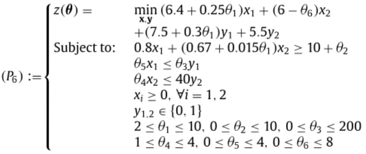
P6

)

:=

⎧

⎪

⎪

⎪

⎪

⎪

⎪

⎪

⎪

⎪

⎪

⎨

⎪

⎪

⎪

⎪

⎪

⎪

⎪

⎪

⎪

⎪

⎩

z

(

θ

)

= min x,y

(

6.4+ 0.25

θ

1

)

x1 +

(

6−

θ

6

)

x2 +

(

7.5+ 0.3

θ

1

)

y1 + 5.5y2 Subjectto: 0.8x1 +

(

0.67+ 0.015

θ

1

)

x2 ≥10+

θ

2

θ

5x1 ≤

θ

3y1

θ

4x2 ≤40y2 xi ≥0,

∀

i= 1,2 y1,2 ∈

{

0,1

}

2 ≤

θ

1 ≤10,0≤

θ

2 ≤10,0 ≤

θ

3 ≤200 1 ≤

θ

4 ≤4,0 ≤

θ

5 ≤4,0 ≤

θ

6 ≤8

The total number of candidate solutions are 8 as shown in Table S.7.

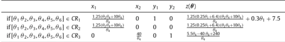
Following the steps of Algorithm1, 4 integer feasible paramet- ric solutions are found and the final ones are 3. Notice, that al- though the number of candidate solutions does not grow, the de- gree of power-products that appear in the optimisers and the La- grange multipliers grows. The final explicit solutions of the case study 1 are given in Table 10 while the corresponding CRs in Table11.

3.6.2. Casestudy2

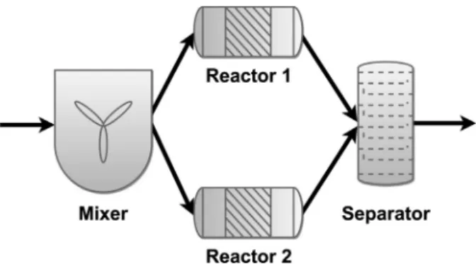
The present case study is a variant of a process synthesis prob- lem adopted from Biegleretal.(1997). Within the synthesis prob- lem, uncertainty in process demand, operation cost and conversion rate, namely

θ

1,

θ

2 and

θ

3, respectively. As shown in figure, the

process refers to the production of a chemical C ( x5) which can

be achieved either through process unit II or III; for the produc- tion of C, a chemical species B ( x2,3) needs to be converted. B, can

be either purchased directly from the market ( x4) or manufactured

through process I with raw material A ( x1) as feed (see Fig.9).

The corresponding MILP under global uncertainty is formulated as an mp-MILP as follows,

(

P7

)

:=

⎧

⎪

⎪

⎪

⎪

⎪

⎪

⎪

⎪

⎪

⎪

⎪

⎪

⎪

⎪

⎪

⎪

⎪

⎪

⎪

⎪

⎪

⎪

⎨

⎪

⎪

⎪

⎪

⎪

⎪

⎪

⎪

⎪

⎪

⎪

⎪

⎪

⎪

⎪

⎪

⎪

⎪

⎪

⎪

⎪

⎪

⎩

z

(

θ

)

= min x,y 2.5x1+

(

4+

θ

1

)

x2+ 5.5x3+ 10y1 +15y2+ 20y3 −18x5 Subjectto: 0.9x1−x2 −x3+ x4 = 0 x5 = 0.82x2 +

θ

3x3 2 ≤x5≤5+

θ

2 x1 ≤16y1 x2 ≤30y2 x3≤30y3 y2+ y3 ≥1 x4 ≤14 0.4x1 ≤5+

θ

2 x_i ≥0,

∀

i = 1,...,5 yi ∈

{

0,1

}

,

∀

i = 1,2,3 0 ≤

θ

1 ≤5 0 ≤

θ

2 ≤5 0.75≤

θ

3 ≤0.95

The LHS uncertainty involved in ( P7) is located in the second

equality constraint and represents uncertainty in the conversion coefficient. Solving problem ( P7) results in 97 candidate solutions.

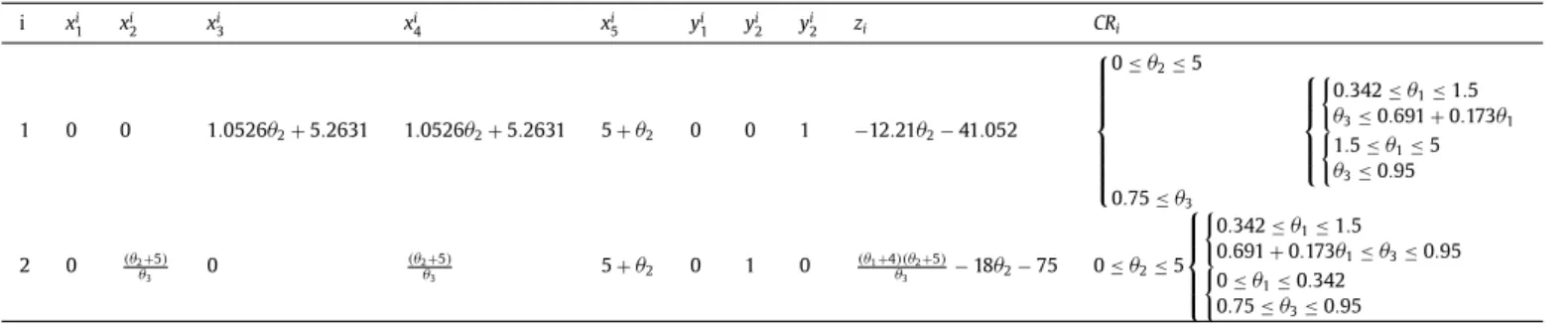
Evaluating with the optimality and integrality conditions results in 3 integer feasible solutions. Two of these solutions are found to overlap and the comparison procedure is employed, resulting in two final optimal solutions which are given in Table12 along with their corresponding CRs.