Technological University Dublin
Technological University Dublin
ARROW@TU Dublin
ARROW@TU Dublin
Articles
School of Mathematics
2015
Efficient Computational Strategies for Doubly Intractable
Efficient Computational Strategies for Doubly Intractable
Problems with Applications to Bayesian Social Networks
Problems with Applications to Bayesian Social Networks
Alberto Caimo
Technological University Dublin, [email protected]
Antonietta Mira
Università della Svizzera Italiana, [email protected]
Follow this and additional works at: https://arrow.tudublin.ie/scschmatart
Part of the Mathematics Commons
Recommended Citation
Recommended Citation
Caimo, A. and Mira, A. (2015). Efficient Computational Strategies for Doubly Intractable Problems with Applications to Bayesian Social Networks. Statistics and Computing, 25(1), 113 – 125, 2015 doi: 10.21427/cn08-ks89
This Article is brought to you for free and open access by the School of Mathematics at ARROW@TU Dublin. It has been accepted for inclusion in Articles by an authorized administrator of ARROW@TU Dublin. For more
information, please contact
[email protected], [email protected], [email protected].
This work is licensed under a Creative Commons Attribution-Noncommercial-Share Alike 3.0 License
1 23
Statistics and Computing
ISSN 0960-3174
Stat Comput
DOI 10.1007/s11222-014-9516-7
Efficient computational strategies
for doubly intractable problems with
applications to Bayesian social networks
1 23
Your article is protected by copyright and all
rights are held exclusively by Springer Science
+Business Media New York. This e-offprint is
for personal use only and shall not be
self-archived in electronic repositories. If you wish
to self-archive your article, please use the
accepted manuscript version for posting on
your own website. You may further deposit
the accepted manuscript version in any
repository, provided it is only made publicly
available 12 months after official publication
or later and provided acknowledgement is
given to the original source of publication
and a link is inserted to the published article
on Springer's website. The link must be
accompanied by the following text: "The final
publication is available at link.springer.com”.
Stat Comput
DOI 10.1007/s11222-014-9516-7
Efficient computational strategies for doubly intractable problems
with applications to Bayesian social networks
Alberto Caimo · Antonietta Mira
Received: 15 March 2014 / Accepted: 6 September 2014 © Springer Science+Business Media New York 2014
Abstract Powerful ideas recently appeared in the litera-ture are adjusted and combined to design improved sam-plers for doubly intractable target distributions with a focus on Bayesian exponential random graph models. Different forms of adaptive Metropolis–Hastings proposals (vertical, horizontal and rectangular) are tested and merged with the delayed rejection (DR) strategy with the aim of reducing the variance of the resulting Markov chain Monte Carlo estima-tors for a given computational time. The DR is modified in order to integrate it within the approximate exchange algo-rithm (AEA) to avoid the computation of intractable nor-malising constant that appears in exponential random graph models. This gives rise to the AEA + DR: a new methodology to sample doubly intractable distributions that dominates the AEA in the Peskun ordering (Peskun Biometrika 60:607– 612, 1973) leading to MCMC estimators with a smaller asymptotic variance. TheBergmpackage forR(Caimo and Friel J. Stat. Softw. 22:518–532,2014) has been updated to incorporate the AEA + DR thus including the possibility of adding a higher stage proposals and different forms of adap-tation.
Keywords Adaptive Metropolis–Hastings proposal· Delayed rejection·Doubly-intractable target·Intractable likelihoods·Markov chain Monte Carlo·Exponential random graphs
A. Caimo (
B
)Institute of Management, University of Lugano, Lugano, Switzerland
e-mail: [email protected] A. Mira
Institute of Finance, University of Lugano, Lugano, Switzerland e-mail: [email protected]
1 Introduction
In this paper we combine the approximate exchange algo-rithm (AEA) proposed inCaimo and Friel(2011), which has been proven to be particularly efficient in estimating expo-nential random graph models (ERGMs), with the delayed rejection (DR) introduced in Tierney and Mira (1999), a strategy to reduce the asymptotic variance of the resulting MCMC estimators. In particular we focus on the adaptive direction sampling approximate exchange algorithm (ADS-AEA) which is based on the idea of running, in parallel, multiple chains that, at each fixed simulation time, interact with each other to allow the construction of a distribution that selects the proposal direction of the candidate move by picking at random a pair of chains.
We also suggest an alternative to ADS-AEA based on an adaptive random walk proposal distribution. Three different adaptation strategies will be studied to design a good proposal variance-covariance matrix: the first one is based on the past history of each single chain (vertical adaptation); the second is based on the current population of all chains at the given simulation time (horizontal adaptation), and finally global adaptation takes into account the past history of all chains (rectangular adaptation).
The three ingredients (ADS, DR and Adaptive proposal) are combined in various ways and compared to obtain the most effective strategy. Optimality is measure by the effective sample size (ESS) and the performance (defined as ESS per simulation time) and the focus is on estimating ERGMs.
The novel methodological contribution consists in the new second (and higher stage) acceptance probability of the approximate exchange algorithm with delayed rejection (AEA + DR) that does not require the calculation of the likeli-hood normalising constant and can thus be used to generate a Markov chain having a general doubly intractable posterior
Author's personal copy
Stat Comput target as its stationary distribution. The DR strategy leads,
by construction, to MCMC estimators that have a smaller asymptotic variance. Indeed the AEA-DR dominates, in the Peskun sense (Peskun 1973), the regular AEA.
2 Exponential random graph models
Exponential random graph models (seeRobins et al.(2007) for a recent review) assume that the topological structure in an observed network y can be explained by the relative prevalence of a set of overlapping sub-graph configurations
s(y)also called graph or network statistics.
Each network statistic has an associated unknown para-meter. A positive value for a certain parameterθ(i)indicates that the edges involved in the formation of the corresponding network statistic si(y)are more likely to be observed relative to edges that are not involved in the formation of that network statistic, and vice versa.
Network statistics and parameters are at the core of ERGMs and the challenge is to estimate the parameters for each statistic such that the model is a good fit for the given data. From a statistical point of view, networks are relational data represented as mathematical graphs. A graph consists of a set of n nodes and a set of m ties which define a relation-ship between pairs of nodes called dyads. The connectivity pattern of a graph can be described by an n×n adjacency
matrix y encoding the presence or absence of a tie between node i and j : yi j =1 if the dyad(i,j)is connected, yi j =0 otherwise. The likelihood of an ERGM represents the prob-ability distribution of a random network graph and can be expressed as:
p(y|θ)= q(y|θ)
z(θ) =
exp{s(y)Tθ}
z(θ) (1)
where q(y|θ)is the unnormalised likelihood. This equation states that the probability of observing a given network graph
y is equal to the exponent of the observed graph statistics s(y)
multiplied by parameter vectorθ divided by a normalising constant term z(θ). The latter is calculated over the sum of all possible graphs on n nodes and it is therefore extremely diffi-cult to evaluate for all but trivially small graphs since this sum involves 2(n2)terms (for undirected graphs). The intractable
normalising constant makes inference difficult for both fre-quentist and Bayesian approaches. This problem does not only occur in ERGMs, but in many other statistical models including, for example, the autologistic model (Besag 1974) in spatial statistics. Given the similarities among these mod-els from a computational tractability point of view, we envis-age that the MCMC simulation strategies proposed in this paper are amenable of successful application in these other contexts as well.
3 Bayesian methods for ERGMs
Bayesian methods are becoming increasingly popular as techniques for modelling social networks. In the ERGM con-text recent works on using the Bayesian approach for infer-ring ERGMs have been proposed byKoskinen et al.(2010) andCaimo and Friel(2011, 2013).
Following the Bayesian paradigm, a prior distribution is assigned toθ. The posterior distribution ofθgiven the data
y is:
p(θ|y)= p(y|θ)p(θ)
p(y) . (2)
Direct evaluation of p(θ|y)requires the calculation of both the likelihood p(y|θ)and the marginal likelihood p(y)which are typically intractable. For this reason posterior parameter estimation for ERGMs has been termed a doubly-intractable problem.
3.1 Exchange algorithm
Markov chain Monte Carlo (MCMC) algorithms (Tierney 1994) are general simulation methods for sampling from posterior distributions and computing posterior quantities of interest. The most widely used MCMC sampler is the Metropolis–Hastings (MH) that, under easy to verify regu-larity conditions, constructs an ergodic Markov chain having the posterior p(θ|y)∝ p(y|θ)p(θ)as its unique stationary and limiting distribution.
A naïve MH update, proposing to move from the cur-rent stateθtoθ1, would require calculation of the following acceptance probability at each sweep of the algorithm:
α(θ, θ1)=1∧ q(y|θ1)p(θ1)h(θ|θ1) q(y|θ)p(θ)h(θ1|θ) × z(θ) z(θ1) (3) where q(·)represents the unnormalised likelihood and h(·)is a proposal distribution used to generate the candidate move
θ1. For doubly intractable target distributions, the ratio in (3) is unworkable due to the presence of the normalising con-stants z(θ)and z(θ1)(note that, on the other hand, the mar-ginal likelihood cancels and thus one source of intractability is resolved).
A special case of the MH algorithm is the random-walk MH, where the proposal (typically a Gaussian distribution) is centred at the current position of the Markov chain and thus
θ1 =θ+σ whereis, usually, a standard Gaussian dis-placement. Since this proposal h is symmetric i.e. h(θ|θ1)=
h(θ1|θ), it cancels in the acceptance ratio. A typical diffi-culty in the MH algorithm is the proper tuning of the pro-posal distribution that translates, for the random-walk MH in the choice of the tuning parameterσ. Off-line tuning aim-ing at achievaim-ing the optimal (in some high dimensional
con-Author's personal copy
Stat Comput
text) acceptance rate of approximately 0.234 (Roberts et al. 1997; Roberts and Rosenthal 1998, 2001) is possible but time consuming. A recent better alternative is adaptive on-line design of the proposal: when tuning the proposal at sim-ulation time t the whole past history of the chain can be taken into account. Different forms of adaptations are possi-ble but since these adaptive strategies destroy the Markovian properties of the sampler, careful rules should be followed in on-line adaptation procedures (Andrieu and Atchadé 2006;
Andrieu and Moulines 2006;Roberts and Rosenthal 2007;
Atchadé and Rosenthal 2005). Another possibility is to run in parallel more Markov chains, all having the same target distribution, and when designing the proposal for one of the chains learn from the current position of the other ones. This strategy does not destroy the Markovian property of the chain being updated and thus it is easier to adopt and gives more freedom in designing adaption strategies, but has additional computational costs. This is the reason why, when compar-ing alternative adaptation strategies, simulation time should be taken into account.
To get around the issue related to the intractability of the likelihood and thus of the MH acceptance probability, Mur-ray et al.(2006) proposed to estimate zz(θ(θ)
1) directly, by
con-sidering the following augmented distribution:
p(θ1,y1, θ|y)∝ p(y|θ)p(θ)h(θ1|θ)×p(y1|θ1) (4) where y1 are auxiliary data generated from the distribu-tion p(·|θ1)which is the same distribution from which the observed data y are assumed to have been sampled from. Notice that the original target is a proper marginal of the augmented distribution thus, running a Markov chain on the augmented state space and marginalising overθ, returns an ergodic sample from the proper posterior of interest.
Using this augmented distribution has the advantage that the acceptance probability in (3) can be written as:
1∧q(y|θ1)p(θ1)h(θ|θ1) q(y|θ)p(θ)h(θ1|θ) × q(y1|θ) q(y1|θ1)× z(θ) z(θ1)× z(θ1) z(θ). (5)
All intractable normalising constants cancel above and below the ratio making the acceptance probability (5) of the Metropolis–Hastings algorithm on the enlarged state space, computable.
3.2 Adaptive direction sampling approximate exchange algorithm (ADS-AEA)
The exchange algorithm of Murray et al. (2006) requires exact simulation of new data y1from the likelihood p(·|θ1). However in the ERGM context, and more generally in Gibbs random fields, exact sampling from the likelihood is difficult.
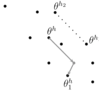
Caimo and Friel(2011) proposed to approximate the exact
θ
h2θ
h1θ
hθ
h1
Fig. 1 The move ofθhis generated from the differenceθh1−θh2plus
a random term
simulation of y1 from p(·|θ1)using MCMC. A theoretical justification for the validity of this approach has been given byEveritt(2012).
In order to improve mixingCaimo and Friel(2011) use an adaptive direction sampling (ADS) method (Gilks et al. 1994;Roberts and Gilks 1994) similar to that ofBraak and Vrugt(2008). The approach consists in running in parallel a collection of H chains which interact with one another. The ADS move (Fig.1), as illustrated inCaimo and Friel(2011), can be described as follows. Set a scalar value forγ (ADS move factor), for each chain h:
(1) Sample two current statesθh1 andθh2 without
replace-ment from the population{1, . . . ,H} \h
(2) Samplefrom a symmetric proposal distribution (3) Proposeθ1h=θh+γθh1−θh2+
(4) Sample y1from p(·|θ1h)
(5) Accept the move fromθhtoθ1hwith probability
α(θh, θh 1)=1∧ q(y|θh 1)p(θ h 1)q(y1|θ h) q(y|θh)p(θh)q(y 1|θ1h) . (6)
Note that, since the ADS proposal distribution is symmetric, it does not appear in the acceptance probability.
3.3 Florentine marriage network
Let us consider, as a toy example, the 16-node Florentine marriage network data concerning the marriage relations between some Florentine families in around 1430 (Padgett and Ansell 1993). The network graph is displayed in Fig.2. We propose to estimate the posterior distribution of the following 3-dimensional ERGM:
q(y|θ)=exp
θ(1)
s1(y)+θ(2)s2(y)+θ(3)s3(y)
(7) where s1(y)= i<jyi j number of edges
s2(y)=i<j<kyi kyj k number of 2-stars
s3(y)=
i<j<l<kyi kyj kylk number of 3-stars.
Author's personal copy
Stat Comput
Fig. 2 Florentine marriage network graph
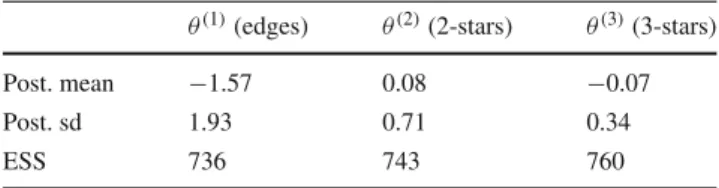
Table 1 Florentine marriage network—Posterior parameter estimates and effective sample size (ESS)
θ(1)(edges) θ(2)(2-stars) θ(3)(3-stars)
Post. mean −1.57 0.08 −0.07
Post. sd 1.93 0.71 0.34
ESS 736 743 760
A vague multivariate Normal prior p(θ) =N(0,100Id)is chosen, where Idis the identity matrix with dimensions equal to that of the model (the same prior setting will be used for all the examples in this paper). TheBergmpackage forR
(Caimo and Friel 2014) allows to carry out inference with the approximate exchange algorithm described above.
We set the ADS move factor γ = 0.8 and =
N(0,0.025Id). The auxiliary chain used to simulate auxil-iary network data from the model consists of 50 iterations and the main chain of 4,000 iterations for each of the 6 chains of the MCMC population so that we have a total of 24,000 main iterations. The tuning parameters were chosen so that the overall acceptance rate is around 21 %. Table1
shows the posterior estimates and effective sample size (ESS) (Kass et al. 1998) which is calculated for each parameterθ(i),
i =1, . . . ,d: E S S θ(i)= S 1+2kρk(θ(i)) ,
where S is the number of posterior samples andρk(·)is the autocorrelation at lag k. The infinite sum is often truncated at lag k whenρk(θ(i)) <0.05.
The results indicate the tendency to a low number of edges as expressed by the edge parameterθ(1)and null parameter values forθ(2)andθ(3). These estimates are consistent with the ones obtained using a frequentist approach (Hunter et al. 2008) as expected given the fairly vague prior.
4 Delayed rejection strategy
Delayed rejection (DR) is a modification of the Metropo-lis-Hastings MCMC algorithm introduced in Tierney and Mira (1999) and generalized in Green and Mira (2001);
Mira(2001a), aimed at improving efficiency of the result-ing MCMC estimators relative to asymptotic variance order-ings introduced inPeskun(1973) and generalized byTierney
(1998);Mira(2001b). The basic idea is that, upon rejection in a MH, instead of advancing simulation time and retaining the same position of the Markov chain, a second stage move is proposed. The acceptance probability of the second stage candidate preserves reversibility of the Markov chain with respect to the target distribution of interest (the posterior, in a Bayesian setting). This delaying rejection mechanism can be iterated for a fixed or random number of stages.
The higher stage proposal distributions can be designed in a very flexible way (using our intuition on the target at hand) and are allowed to depend not only on the current position of the Markov chain but also on the candidates so far proposed and rejected (within each sweep). In some sense we can learn from our earlier mistakes. But notice that this form of local adaptation does not destroy the Markovian property since, as soon as a candidate move is accepted, the rejected val-ues are disregarded. Thus DR allows partial local adaptation of the proposal within each time step of the Markov chain still retaining reversibility and Markovianity. The advantage of DR over alternative ways of combining different MH pro-posals or kernels, such as mixing and cycling (Tierney 1994), is that a hierarchy between kernels can be exploited so that kernels that are easier to compute (in terms of CPU time) are tried first, thus saving in terms of simulation time. Or moves that are more “bold” (bigger variance of the proposal, for example) are tried at earlier stages thus allowing the sampler to explore the state space more efficiently following a sort of “first bold” versus “second timid” tennis-service strategy.
Suppose the current position of the Markov chain is Xt =
θ. As in a regular MH, a candidate moveθ1is generated from a proposal h1(θ,·)and accepted with probability
α1(θ, θ1)=1∧ p(θ1,y)h1(θ1|θ)
p(θ,y)h1(θ|θ1) = 1∧ N1
D1.
(8)
Note that the subscript in h1andα1indicate that this is the first stage proposal and acceptance probability. Upon rejec-tion, instead of retaining the same posirejec-tion, Xt+1=θ, as we would do in a standard MH, a second stage moveθ2is gen-erated from a proposal distribution that is allowed to depend, not only on the current position of the chain, but also on what we have just proposed and rejected: h2(θ2|θ, θ1). The second
Author's personal copy
Stat Comput
stage acceptance probability is:
α2(θ, θ1, θ2) =1∧ p(θ2,y)h1(θ1|θ2)h2(θ|θ2, θ1)[1−α1(θ2, θ1)] p(θ,y)h1(θ1|θ)h2(θ2|θ, θ1)[1−α1(θ, θ1)] =1∧ N2 D2. (9) This process of delaying rejection can be iterated and the i -th stage acceptance probability is, followingMira(2001a):
αi(θ, θ1. . . θi)= =1∧Ni Di =1∧ p(θi,y)h1(θi−1|θi)h2(θi−2|θi, θi−1) . . .hi(θ|θi, θi−1. . . θ1) p(θ,y)h1(θ1|θ)h2(θ2|θ, θ1) . . .hi(θi|θ, θ1. . . θi−1) ×[1−α1(θi, θi−1)][1−α2(θi, θi−1, θi−2)]. . .[1−αi−1(θi, . . . , θ1)] [1−α1(θ, θ1)][1−α2(θ, θ1, θ2)]. . .[1−αi−1(θ, θ1, . . . , θi−1)] (10) If the i -th stage is reached, it means that Nj <Dj for j = 1, . . . ,i−1, thereforeαj(θ, θ1. . . θj)is simply Nj/Dj, j = 1, . . . ,i−1 and a recursive formula can be obtained: Di =
hi(θ . . . θi)(Di−1−Ni−1)which leads to:
Di =hi(θi|θ . . .)[hi−1(θi−1|θ . . .)[hi−2(θi−2|θ . . .)· · ·
[h2(θ2,|θ, θ1)[h1(θ1|θ)p(θ,y)−N1] −N2]
−N3]. . .−Ni−1]. (11)
Since reversibility with respect to p is preserved separately at each stage, the process of delaying rejection can be inter-rupted at any stage. The user can either decide, in advance, to try at most, a fixed number of times to move away from the current position or, alternatively, upon each rejection, toss a
π-coin (i.e. a coin with head probability equal toπ), and if the outcome is head move to a higher stage proposal, otherwise stay put.
Tierney and Mira(1999) prove that the DR strategy pro-vides MCMC estimators with smaller asymptotic variance than standard MH. This better performance holds no mat-ter what is the function f whose expectation relative to the target posterior we want to estimate (provided f is squared integrable with respect to the target). The performance of the approach has to be evaluated by weighting the improved asymptotic variance against the increased computational cost of the delayed rejection approach.
5 Approximate exchange algorithm with delayed rejection (AEA + DR)
The idea is to combine the DR strategy with the approximate exchange algorithm. We name this new algorithm the AEA + DR and different instances of it will be specified in subse-quent sections depending of the (adaptive) proposal
distrib-ution used. For the AEA + DR algorithm a theoretical modi-fication of the i -th stage acceptance probability is needed to take into account the fact that the target normalising constant depends on the parameter of interest. This is a novel method-ological contribution that gives rise to an efficient MCMC sampler that can be used in general for doubly intractable problems. Efficiency is measure by the asymptotic variance of the resulting estimators. Indeed the AEA + DR domi-nates, in the Peskun sense (Peskun 1973), the original AEA in that the probability of moving away from the current posi-tion is higher. Indeed, the intuiposi-tion behind Peskun ordering is that, every time a Markov chain, used for MCMC purposes, retains the same position, it fails to explore the state space and the autocorrelation along its path increases, leading to a larger asymptotic variance of the sample path ergodic aver-ages (the MCMC estimators). In a Metropolis–Hastings type algorithm the Markov chain stays put every time a candidate move is rejected. Thus, upon rejection, instead of advancing simulation time and retaining the same position, a second stage move is proposed. This attempt, by itself, increases the probability of moving away from the current position and thus the resulting AEA+DR algorithm achieves higher efficiency as measured by the effective sample size. Since the mechanism of delaying rejection is time consuming, a fair comparison should be made taking simulation time into account and thus considering the performance defined as ESS divided by simulation time.
The first stage acceptance probability is unchanged rela-tive to the standard AEA, and (recalling (5)) is given by:
α1(θ, θ1)=1∧ q(y|θ
1)p(θ1)h1(θ|θ1)q(y1|θ)
q(y|θ) p(θ)h1(θ1|θ)q(y1|θ1)
(12)
The second stage acceptance probability that preserves the detailed balance condition is:
α2(θ, θ1, θ2)
=1∧ q(y|θ2) p(θ2)h1(θ1|θ2)h2(θ|θ2, θ1)q(y2|θ)[1−] q(y|θ)p(θ)h1(θ1|θ)h2(θ2|θ, θ1)q(y2|θ2)[1−α1(θ, θ1)]
(13)
where y2are auxiliary data generated from the distribution
p(·|θ2)which is the same likelihood distribution from which the observed data y are assumed to have been sampled from. Higher stage acceptance probabilities are modified accord-ingly. The second stage proposal of the delayed rejection ver-sion of the adaptive direction sampler (named ADS + DR) is designed to be negatively correlated with the first stage pro-posal following the idea of antithetic second stage suggested inBédard et al.(2010).
Stat Comput 6 Adaptive approximate exchange algorithm (AAEA)
Three forms of adaptation of the Metropolis–Hastings pro-posal distribution (alternative to the ADS-AEA) are consid-ered: vertical, horizontal and rectangular. At simulation time
t there is a rectangular t×H family of particles available: θi,j,i =1, . . . ,t; j=1, . . . ,H . Suppose we are interested in updating the position of particleθt,h(in the previous for-mulas this particle was simply indicated asθ with no sub-scripts). To this aim a random walk Metropolis–Hastings proposal is designed by taking a Gaussian distribution with mean equal toθt,hand variance-covariance matrix, given by the empirical variance (multiplied by 2.382/d where d is the model dimension, followingRoberts and Rosenthal(2009)) of either:
AAEA-1 all past particles along the same chain h (vertical adaptation):θi,h,i =1, . . . ,t−1;
AAEA-2 all particles at the current time t for all chains (hor-izontal adaptation):θt,i,i=1, . . . ,H ;
AAEA-3 particles from all chains and all past simulations (rectangular adaptation, aka inter-chain adaptation fromCraiu et al. 2009) :θi,j,i =1, . . . ,t−1;j = 1, . . . ,H .
The sample covariance matrix used in AAEA-1 and AAEA-3 is computed recursively following the Eq. (3) in
Haario et al.(2001).Roberts and Rosenthal(2007) provide two conditions (“Containment” and “Diminishing Adap-tation”) that guarantee that a generic adaptive MCMC is ergodic with respect to the proper stationary distribution. In order to meet these conditions we follow the algorithm suggested in Roberts and Rosenthal (2007) that, with a small probability β (set equal to 0.01 in our simulation study), instead of using the adaptive proposal described above, uses the following static proposal: Normal distri-bution with variance-covariance matrix equal to 0.0025Id where Id is the identity matrix of size d, the model dimension.
We note that, when designing adaptive algorithms, it is usually not difficult to ensure directly that “Diminish-ing Adaptation” holds, since adaption is user controlled one can always adapt less and less as the algorithm pro-ceeds. However, “Containment” is a technical condition that avoids “escape to infinity”. It always holds, for example, if the target has sub-exponential tails, or if the state space is finite or compact. The latter requirement is easily met by using a prior with compact support which is more than justified in the context of ERGM given the interpretation of the parameters. The “Containment” condition, in gen-eral settings, may be more challenging to check. A careful review of sufficient conditions that ensure it can be found in Bai et al. (2009). We note that the horizontal
adapta-tion scheme described above does not destroy the Markov-ian property since the covarMarkov-iance matrix is updated only based on information available at the current simulation time.
More sophisticated forms of MCMC adaptive strategies could be used in the context of doubly intractable targets. We have not explored them further since, in the context of ERGMs, the adaptation procedures used, despite being sim-ple are quite effective. We refer the interested reader to the tutorial byAndrieu and Thoms(2008) for a general frame-work of stochastic approximation which allows one to sys-tematically optimise generally used criteria for designing adaptive MCMC algorithms, such as targeting a user speci-fied acceptance probability.
As also discussed inCraiu et al.(2009), a question of inter-est in adaptive MCMC is whether one should wait a short or a long time before starting the adaptation. Based on our simu-lation experience we found that the most effective strategy is to use the ADS approach during the burn-in phase and then switch to one of the adaptive algorithm mentioned above. Furthermore, the simulation results presented use intensive adaptation (Giordani and Kohn 2010) i.e. adaptation is per-formed at every iteration.
We believe that more sophisticated forms of adaptations such as regional or tempered adaptation (Craiu et al. 2009) are not needed in our setting.
7 Adaptive approximate exchange algorithm with delayed rejection (AAEA + DR)
The three adaptation schemes outlined in the previous sec-tion could be combined within the DR mechanism. For example at first stage horizontal adaptation can be used since the resulting proposal is typically less computation-ally intensive to obtain (because H is usucomputation-ally smaller than
t especially after the burn-in phase), at second stage we
can try vertical adaptation and resort to rectangular adap-tation only at third stage. The intuition behind this combi-nation is to use simple proposals first and resort to more refined proposals (typically more computationally inten-sive to construct, as rectangular adaptation) only if really needed.
In the examples considered we follow a different rationale when combining the adaptive approximate exchange algo-rithm with the delayed rejection, namely, the second stage proposal is equal to the first stage one with the variance-covariance matrix rescaled by a factor of 0.5. In other words a more timid move is attempted at second stage. This is a very naïve form of delayed rejection but it is often quite effective (see for exampleGreen and Mira(2001);Haario et al.(2006)).
Stat Comput 8 Examples
8.1 Introduction to the results
In this section we compare the adaptive direction sampler (ADS-AEA) with three alternative forms of adaptation as defined in Sect.6.
For each one of the four adaptive algorithms considered we have also implemented the corresponding two stage DR version as explained in Sect.5. For vertical, horizontal and rectangular adaptation this is done by simply adding a second stage proposal which is identical to the first stage one except that the variance-covariance matrix is multiplied by 0.5. For the DR version of the adaptive direction sampler, upon rejection of the first stage candidate move θ1h = θh +
γ1 θh1 1 −θ h2 1
+1, the second stage proposal is deter-ministically obtained from the first one by simply going in the opposite direction relative to the current position:θ2h =
θh−γ 1
θh1−θh2+
1or, in other terms,θ2h=2θ0h−θ1h. This strategy follows the idea of second stage antithetic pro-posal which has been proved in (Bédard et al. 2010) to be generally highly effective.
We thus have a total of eight different algorithms under comparison. To our surprise the horizontal adaptation approach AAEA-2 outperforms all other adaptive algorithms (we were expecting rectangular adaptation to have a better performance given that more particles are used to learn the variance-covariance structure of the target distribution that is then used in the random walk Metropolis–Hastings sam-pler). The performance of the horizontal adaptive algorithms is then further enhanced when combined with the delayed rejection strategy.
The DR version of each algorithm is always better than the corresponding single stage proposal in terms of ESS. This simply confirms the fact that the DR dominates the cor-responding single stage Metropolis–Hastings sampler in the Peskun ordering i.e. in terms of asymptotic variance of the resulting MCMC estimators (for a given number of sweeps). If the additional simulation time of the DR is also taken into account in the comparison (i.e. if we consider the ESS per unit computational time), the DR still outperforms the corre-sponding single stage proposal in all cases but for the adaptive direction sampler (this is because the second stage proposal of the adaptive direction sampler, ADS + DR, has a very small acceptance probability due to the structure of the first stage proposal and the antithetic move implemented at sec-ond stage).
In the next three subsections we present three examples of increasing complexity. The Florentine Marriage Network has 16 nodes and the proposed ERGM has three parameters; the Karate Club network has 34 nodes and three parameters; while the Faux Mesa High School Network has 208 nodes
and nine parameters. We anticipate that, as the dimensions and the complexity of the model increase, the efficiency of the three proposed adaptive strategies with delayed rejection (that turn out to be the winning strategies) becomes more and more comparable in terms performance while, in terms of ESS (a more neutral measure in that it is not affected by coding ability), the best algorithm is rectangular adaptation with delayed rejection.
Horizontal adaptation performs better because calculat-ing the covariance of a small set of points is cheaper than calculating the covariance matrix in vertical and rectangu-lar adaptation where more points enter in the estimation of the covariance. Indeed the CPU time needed to run the three adaptation scheme follows, in general, this ordering CPU-horizontal <CPY-vertical < CPU-rectangular and this is because, when computing the variance-covariance matrix, there and increasingly more particles entering the computa-tion for vertical versus horizontal and for rectangular versus vertical. Furthermore, the number of particles used in vertical and rectangular adaptation increases with simulation length while it is a static value (equal to the number of chains) for horizontal adaptation. Of course the intuition is that more par-ticles lead to a better estimate and thus more efficient sampler resulting in larger ESS. There is thus a trade-off that leads to a competitive advantage of horizontal adaptation in small and simple models. This advantage washes out for larger and more complex models.
Horizontal adaptation performs better for targets of small dimension, because calculating the covariance matrix of a small set of points turns out to be cheaper (in terms of CPU time) than computing the covariance in vertical and rectan-gular adaptation. There is, of course, an interplay between the number of chains and the number of iterations used. In horizontal adaptation, the number of chains has to be “large enough” in order to have the population points spread about the target distribution. As a rule of thumb, in horizontal adap-tation, the number of chains should grow with the square of the dimension of the target since we need to estimate its d dimensional covariance matrix. Thus we conjecture that the better performance of horizontal adaptation will wash out as d grows (more network statistics) and the computational complexity of the problem increases (more nodes), indeed our simulation results agree with this intuition (see results in the last example).
8.2 Florentine marriage network
Let us consider again the Florentine marriage network and model defined in Eq.7. We use a total number of 24,000 iter-ations for estimating the posterior density and four different approaches:
– ADS-AEA consists of six chains of 4,000 iterations each;
Author's personal copy
Stat Comput Table 2 Florentine marriage network—Posterior parameter estimates
and effective sample size (ESS) for model7
θ(1)(edges) θ(2)(2-stars) θ(3)(3-stars)
AAEA-2 (horizontal adaptation)
Post. mean −1.47 0.05 −0.06
Post. sd 1.86 0.69 0.36
AAEA-2+DR (horizontal adaptation + DR)
Post. mean −1.61 0.08 −0.06 Post. sd 1.55 0.53 0.25 1 (edges) -5 0 5 0.00 0.10 0.20 2 (kstar2) -3 -2 -1 0 1 2 3 0.0 0.2 0.4 0.6 3 (kstar3) -2 -1 0 1 0.0 0 .4 0. 8 1.2 0 10 20 30 40 50 -1.0 -0.5 0.0 0 .5 1.0 Lag 0 10 20 30 40 50 -1.0 -0.5 0.0 0 .5 1.0 Lag 0 10 20 30 40 50 -1.0 -0.5 0.0 0.5 1.0 Lag
Fig. 3 Florentine marriage network. MCMC diagnostics for the overall chain. The 2 plot columns are: estimated marginal posterior densities (left), and autocorrelation plots (right)
– AAEA-1 (vertical adaptation) consists of six chains of 4,000 iterations each;
– AAEA-2 (horizontal adaptation) consisting of 24 chains of 1,000 iterations each;
– AAEA-3 (rectangular adaptation) consisting of six chains of 4,000 iterations each.
In Table2are displayed the posterior parameter estimates and effective sample size calculated for the AAEA-2 and
1 (edges) -8 -6 -4 -2 0 2 4 6 0.00 0.10 0.20 2 (kstar2) -2 -1 0 1 2 0.0 0.2 0.4 0 .6 0.8 3 (kstar3) -1.5 -1.0 -0.5 0.0 0.5 1.0 0.0 0.5 1.0 1.5 0 10 20 30 40 50 -1.0 -0.5 0.0 0 .5 1.0 Lag 0 10 20 30 40 50 -1.0 -0.5 0.0 0 .5 1.0 Lag 0 10 20 30 40 50 -1.0 -0.5 0.0 0.5 1.0 Lag
Fig. 4 Florentine marriage network—MCMC diagnostics for the AAEA-2 + DR
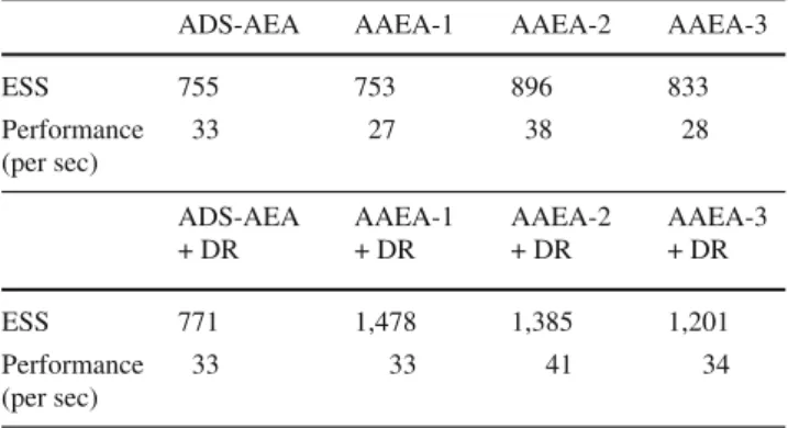
AAEA-2 + DR which turned out to be the best approaches in terms of performance. In particular the AAEA-2 + DR yields a variance reduction of about 83 % compared to the ADS-AEA.
In Fig. 3 it can be seen that the autocorrelations of the parameter estimates returned by the ADS-AEA decay slower than the autocorrelations of the AAEA-2 + DR displayed in Fig.4. The AAEA-2 algorithm outperforms the ADS-AEA in terms of both ESS (20 %) and performance (20 %). The AAEA-2 + DR outperforms the AAEA-2 in terms of ESS of about 60 % and performance of about 15 % (Table3). Computing times can be calculated as ESS / Performance.
In Table4it is possible to observe the correlation matrix between the parameters in the posterior distribution. There is a very strong negative correlation between all the parameters of the model.
8.3 Karate club network
This example concerns the karate club network (Zachary 1977) displayed in Fig.5which represents friendship
rela-Author's personal copy
Stat Comput
Table 3 Florentine marriage network—effective sample size (ESS) and performance for each algorithm for model7based on 100 simulations
ADS-AEA AAEA-1 AAEA-2 AAEA-3
ESS 755 753 896 833 Performance (per sec) 33 27 38 28 ADS-AEA + DR AAEA-1 + DR AAEA-2 + DR AAEA-3 + DR ESS 771 1,478 1,385 1,201 Performance (per sec) 33 33 41 34
Table 4 Florentine marriage network—Posterior correlation matrix between the parameters in the distribution for model7
θ(1) θ(2) θ(3)
θ(1) 1.00 −0.94 −0.80
θ(2) – 1.00 −0.94
θ(3) – − 1.00
tions between 34 members of a karate club at a US university in the 1970.
We propose to estimate the following 3-dimensional model using the network statistics proposed bySnijders et al.(2006):
q(y|θ)=exp
θ(1)
s1(y)+θ(2)v(y, φu)+θ(3)u(y, φv)
(14) where s1(y)= i<j yi jnumber of edges v(y, φv)=eφvn−2 i=1 1−1−e−φvi E Pi(y) geometrically weighted edgewise shared partners
(GWESP) u(y, φu)=eφu n−1 i=1 1−1−e−φui Di(y) geometrically weighted degrees (GWD)
where E Pi(y)and Di(y)are the edgewise shared partners and degree distributions respectively. We setφu = φv = log(2)so that the model is a non-curved ERGM (Hunter and Handcock 2006). The prior setting is the same as the one in Sect.3.3: p(θ) = N(0,100I3). The tuning parameters for the ADS proposal are:γ =0.9 and = N(0,0.0025Id)so that the overall acceptance rate is around 21 %. The auxiliary chain consists of 100 iterations and a total number of 24,000 main iterations is used. The number of chains used in the
Fig. 5 Zachary karate club network graph
Table 5 Zachary karate club network—Posterior parameter estimates for model14
θ(1)(edges) θ(2)(gwesp) θ(3)(gwdegree)
ADS-AEA
Post. mean −3.51 0.74 1.18
Post. sd 0.62 0.21 1.12
AAEA-2+DR (horizontal adaptation + DR)
Post. mean −3.44 0.72 1.01
Post. sd 0.59 0.21 1.07
various strategies is the same as in the previous example in Sect.8.2.
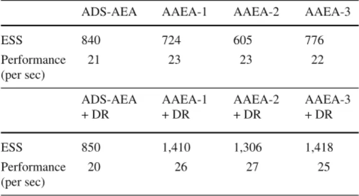
In Table5are displayed the posterior parameter estimates obtained using the ADS-AEA and AAEA-2 + DR. In this example, as happened in the teenage friendship network above, the AAEA-3 outperforms the AAEA-2 in terms of variance reduction of about 40 % but not in terms of per-formance. For this reason AAEA-2 is still to be preferred (Fig.6).
In Fig. 7 it can be seen that the autocorrelations of the parameters for the AAEA-2 approach decay quicker than the autocorrelations given by the other methods as shown in Fig.6. The AAEA-2 outperforms the ADS-AEA of about 12 % in terms of performance whereas the AAEA-2 + DR makes a further improvement of about 20 % with respect to the AAEA-2 + DR (see Table6).
As in the Florentine marriage network example, we can observe (Table 7) that there is a strong negative posterior correlation between parameters θ(1) andθ(2) and between
θ(1)andθ(3).
Generally a strong correlation between parameters in the posterior distribution hampers the behaviour of vanilla MCMC schemes. In fact high posterior correlation can slow down the motion of the chain towards equilibrium distribu-tion. It is in this case that the adaptive approximate exchange algorithm with delayed rejection (AAEA-2 + DR) gives the best performance compared to the adaptive direction sam-pling approximate exchange algorithm.
Stat Comput 1 (edges) -6 -5 -4 -3 -2 -1 0 0.0 0.1 0.2 0.3 0.4 0.5 2 (gwesp.fixed.0.693147180559945) -0.5 0.0 0.5 1.0 1.5 0.0 0.5 1.0 1.5 3 (gwdegree) -4 -2 0 2 4 6 8 0.00 0.10 0.20 0.30 0 10 20 30 40 50 -1.0 -0.5 0.0 0.5 1.0 Lag 0 10 20 30 40 50 -1.0 -0.5 0.0 0.5 1.0 Lag 0 10 20 30 40 50 -1.0 -0.5 0.0 0.5 1.0 Lag
Fig. 6 Zachary karate club network—MCMC diagnostics for the ADS-AEA
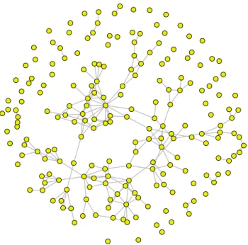
8.4 Faux Mesa high school network
In this example we revisit a well known network dataset (Fig.8) in social science concerning friendship relations in a school community of 203 students (Handcock et al. 2007). The vertex attributes x that we are interested in are “grade” (it takes values 7 through 12 indicating each student’s grade in school) and “sex” of each student.
The main focus is on the factor attribute effects (which give information about the tendency of a node with a specific attribute to form an edge in the network) and on the transi-tivity effect expressed by the GWESP and GWD statistics defined in Sect. 8.3withφu=φv=1.
The model we propose to estimate is defined by the fol-lowing nine network statistics:
s1(y)= i<jyi jnumber of edges s2(y,x)= i<jyi j(1(gr adei=8)+1(gr adej=8)) node factor for “grade”=8
s3(y,x)= i<jyi j(1(gr adei=9)+1(gr adej=9)) 1 (edges) -6 -5 -4 -3 -2 0.0 0.2 0.4 0.6 2 (gwesp.fixed.0.693147180559945) 0.0 0.5 1.0 1.5 0.0 0.5 1.0 1.5 2.0 3 (gwdegree) -2 0 2 4 6 0.0 0.1 0.2 0.3 0.4 0 10 20 30 40 50 -1.0 -0.5 0.0 0.5 1.0 Lag 0 10 20 30 40 50 -1.0 -0.5 0.0 0.5 1.0 Lag 0 10 20 30 40 50 -1.0 -0.5 0.0 0.5 1.0 Lag
Fig. 7 Zachary karate club network—MCMC diagnostics for the AAEA-2 + DR
Table 6 Zachary karate club network—effective sample size (ESS) and performance for each algorithm for model14based on 100 simulations
ADS-AEA AAEA-1 AAEA-2 AAEA-3
ESS 840 724 605 776 Performance (per sec) 21 23 23 22 ADS-AEA + DR AAEA-1 + DR AAEA-2 + DR AAEA-3 + DR ESS 850 1,410 1,306 1,418 Performance (per sec) 20 26 27 25
Table 7 Zachary karate club network—Posterior correlation matrix between the parameters in the distribution for model14
θ(1) θ(2) θ(3)
θ(1) 1.00 −0.80 −0.75
θ(2) – 1.00 0.37
θ(3) – – 1.00
Stat Comput
Fig. 8 Faux Mesa High School friendship network graph
node factor for “grade”=9
s4(y,x)=
i<jyi j(1(gr edei=10)+1(gr adej=10)) node factor for “grade”=10
s5(y,x)=
i<jyi j(1(gr adei=11)+1(gr adej=11)) node factor for “grade”=11
s6(y,x)=
i<jyi j(1(gr adei=12)+1(gr adej=12)) node factor for “grade”=12
s7(y,x)=
i<jyi j(1(sexi=M)+1(sexj=M)) node factor for “sex = male”
s8(y)=v(y, φv)GWESP
s9(y)=u(y, φu)GWD
where1(·)is the indicator function.
The tuning parameters for the ADS proposalγ =0.3 and
= N(0,0.0025Id)are chosen so as to obtain the overall acceptance rate is around 21 %. 5,000 auxiliary iterations are
used for network simulation and 60,000 main iterations are used for estimating the posterior density of model defined above:
– ADS-AEA consists of 20 chains of 3,000 iterations each; – AAEA-1 (vertical adaptation) consists of 30 chains of
2,000 iterations each;
– AAEA-2 (horizontal adaptation) consists of 20 chains of 3,000 iterations each;
– AAEA-3 (rectangular adaptation) consists of 20 chains of 3,000 iterations each.
In Table8are displayed the posterior parameter estimates obtained using the ADS-AEA and AAEA-2 + DR. In Table9, the adaptive algorithms with delayed rejection outperform the ADS-AEA in terms of both variance reduction and per-formance. All the adaptive algorithms with delayed rejection deliver the same results in terms of performance.
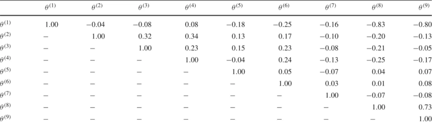
As in the previous examples, we can observe (Table10) that there is a strong negative posterior correlation between parametersθ(1)andθ(8)and betweenθ(1)andθ(9).
From the results displayed in Table8we can conclude that the network is very sparse (θ(1)negative) and that students having the same gender seem to create friendship connections (θ(7)negative). The transitivity effect expressed byθ(8)and the popularity effect expressed byθ(9)are important features of the network.
9 Conclusions
The exchange algorithm of Murray et al. (2006) makes the computation of the MH acceptance probability feasi-ble even for target distributions whose normalizing con-stant depends on the parameter of interest (doubly intractable problems).
The approximate exchange algorithm, due toCaimo and Friel(2011), modifies the original exchange algorithm and makes it applicable also in settings where sampling from the assumed data generating process is not feasible. This is the case for exponential random graphs the model we focus on in this paper.
Table 8 Faux Mesa High School network—Posterior parameter estimates θ(1) θ(2) θ(3) θ(4) θ(5) θ(6) θ(7) θ(8) θ(9) ADS-AEA Post. mean −5.53 −0.15 −0.09 −0.04 −0.12 0.20 −0.18 0.28 1.53 Post. sd 0.33 0.15 0.17 0.21 0.18 0.23 0.12 0.25 0.12 AAEA-2 + DR (horizontal adaptation + DR)
Post. mean −5.48 −0.14 −0.09 −0.04 −0.11 0.19 −0.17 0.27 1.52 Post. sd 0.30 0.12 0.13 0.19 0.16 0.20 0.10 0.23 0.11
Stat Comput Table 9 Faux Mesa High
School network—ESS and performance for each algorithm based on 10 simulations
ADS-AEA AAEA-1 AAEA-2 AAEA-3
ESS 667 1,041 1,008 1,094
Performance (per sec) 1.8 2.3 2.1 2.2
ADS-AEA+DR AAEA-1 + DR AAEA-2 + DR AAEA-3 + DR
ESS 873 1,376 1,320 1,440
Performance (per sec) 1.4 2.6 2.6 2.6
Table 10 Faux Mesa High School network—Posterior correlation matrix between the parameters
θ(1) θ(2) θ(3) θ(4) θ(5) θ(6) θ(7) θ(8) θ(9) θ(1) 1.00 −0.04 −0.08 0.08 −0.18 −0.25 −0.16 −0.83 −0.80 θ(2) − 1.00 0.32 0.34 0.13 0.17 −0.10 −0.20 −0.13 θ(3) − − 1.00 0.23 0.15 0.23 −0.08 −0.21 −0.05 θ(4) − − − 1.00 −0.04 0.24 −0.13 −0.25 −0.17 θ(5) − − − − 1.00 0.05 −0.07 0.04 0.07 θ(6) − − − − − 1.00 0.03 0.01 0.08 θ(7) − − − − − − 1.00 −0.07 −0.08 θ(8) − − − − − − − 1.00 0.73 θ(9) − − − − − − − − 1.00
The delayed rejection strategy allows to locally adapt the proposal distribution within each sweep of a MH algorithm at the cost of additional computational time.
The adaptive random walk proposal ofHaario et al.(2001) revised byRoberts and Rosenthal(2009) allows for global adaptation between MH iterations. This learning from the past process is also expensive from a computational point of view.
These three ingredients are combined in different ways within the approximate exchange algorithm (AEA) to avoid the computation of intractable normalising constant that appears in exponential random graph models. This gives rise to the AEA + DR: a new methodology to sample dou-bly intractable target distributions which achieves variance reduction relative to the adaptive direction sampling approx-imate exchange algorithm ofCaimo and Friel(2011) imple-mented in theBergmpackage forR(Caimo and Friel 2014), which is our benchmark.
The 8 algorithms under comparison (seven of which are original contributions) are tested on three examples. Consis-tently, the best combination (in terms of ESS for fixed simu-lation time), is given by the horizontal adaptive approximate
exchange algorithm with delayed rejection, which achieves a
variance reduction that varies between 55 and 98 % (relative to the benchmark).
This translates into a better performance varying from 25 to 40 %, if the extra simulation time, due to the delayed rejection mechanism and the adaptation procedure, is taken
into account. The strongest improvements are obtained in the examples with highly correlated posterior distributions.
The applicability of the proposed methodology goes beyond the social network context as it works for any doubly intractable target.
The delayed rejection strategy and the form of adaptation proposed in the present paper have been implemented in the
Bergmpackage.
Acknowledgments The authors gratefully acknowledge financial
support from the Swiss National Science Foundation.
References
Andrieu, C., Atchadé, Y.F.: On the efficiency of adaptive MCMC algo-rithms. In: Proceedings of the 1st International Conference on Performance Evaluation Methodologies and Tools, ACM Inter-national Conference Proceeding Series, vol. 180 (2006) Andrieu, C., Moulines, É., et al.: On the ergodicity properties of some
adaptive MCMC algorithms. Ann. Appl. Probab. 16(3), 1462– 1505 (2006)
Andrieu, C., Thoms, J.: A tutorial on adaptive MCMC. Stat. Comput. 18(4), 343–373 (2008)
Atchadé, Y.F., Rosenthal, J.S., et al.: On adaptive Markov chain Monte Carlo algorithms. Bernoulli 11(5), 815–828 (2005)
Bai, Y., Roberts, G.O., Rosenthal, J.S.: On the containment condition for adaptive Markov chain Monte Carlo algorithms. Adv. Appl. Stat. 21, 1–54 (2009)
Bédard, M., Douc, R., Moulines, E.: Scaling analysis of delayed rejec-tion MCMC methods. Methodol. Comput. Appl. Probab. 29, 1–28 (2010)
Stat Comput
Besag, J.E.: Spatial interaction and the statistical analysis of lattice systems (with discussion). J. R. Stat. Soc. Ser. B 36, 192–236 (1974)
Caimo, A., Friel, N.: Bayesian inference for exponential random graph models. Soc. Netw. 33(1), 41–55 (2011)
Caimo, A., Friel, N.: Bayesian model selection for exponential random graph models. Soc. Netw. 35(1), 11–24 (2013)
Caimo, A., Friel, N.: Bergm: Bayesian exponential random graphs in R. J. Stat. Softw. (2014), to appear
Craiu, R.V., Rosenthal, J., Yang, C.: Learn from thy neighbor: parallel-chain and regional adaptive MCMC. J. Am. Stat. Assoc. 104(488), 1454–1466 (2009)
Everitt, R.G.: Bayesian parameter estimation for latent Markov random fields and social networks. J. Comput. Graph. Stat. 21(4), 940–960 (2012)
Gilks, W.R., Roberts, G.O., George, E.I.: Adaptive direction sampling. Statistician 43(1), 179–189 (1994)
Giordani, P., Kohn, R.: Adaptive independent Metropolis–Hastings by fast estimation of mixtures of normals. J. Comput. Graph. Stat. 19(2), 243–259 (2010)
Green, P.J., Mira, A.: Delayed rejection in reversible jump Metropolis– Hastings. Biometrika 88(4), 1035–1053 (2001)
Haario, H., Saksman, E., Tamminen, J.: An adaptive Metropolis algo-rithm. Bernoulli 7(2), 223–242 (2001)
Haario, H., Laine, M., Mira, A., Saksman, E.: Dram: efficient adaptive MCMC. Stat. Comput. 16(4), 339–354 (2006)
Handcock, M.S., Hunter, D.R., Butts, C.T., Goodreau, S.M., Morris, M.: Statnet: software tools for the representation, visualization, analysis and simulation of network data. J. Stat. Softw. 24(1):1– 11, (2007)http://www.jstatsoft.org/v24/i01
Hunter, D.R., Handcock, M.S., Butts, C.T., Goodreau, S.M., Morris, M.: Ergm: A package to fit, simulate and diagnose exponential-family models for networks. J. Stat. Softw. 24(3):1–29, (2008)
http://www.jstatsoft.org/v24/i03
Hunter, D.R., Handcock, M.S.: Inference in curved exponential family models for networks. J. Comput. Graph. Stat. 15, 565–583 (2006) Kass, R.E., Carlin, B.P., Gelman, A., Neal, R.M.: Markov chain Monte Carlo in practice: a roundtable discussion. Am. Stat. 52(2), 93–100 (1998)
Koskinen, J.H., Robins, G.L., Pattison, P.E.: Analysing exponential ran-dom graph (p-star) models with missing data using Bayesian data augmentation. Stat. Methodol. 7(3), 366–384 (2010)
Mira, A.: On Metropolis–Hastings algorithms with delayed rejection. Metron 59(3–4), 231–241 (2001a)
Mira, A.: Ordering and improving the performance of Monte Carlo Markov chains. Stat. Sci. 16, 340–350 (2001b)
Murray, I., Ghahramani, Z., MacKay, D.: MCMC for doubly-intractable distributions. In: Proceedings of the 22nd Annual Conference on Uncertainty in Artificial Intelligence (UAI-06), AUAI Press, Arlington (2006)
Padgett, J.F., Ansell, C.K.: Robust action and the rise of the Medici, 14001434. Am. J. Sociol. 98(12591), 319 (1993)
Peskun, P.: Optimum Monte-Carlo sampling using Markov chains. Bio-metrika 60(3), 607–612 (1973)
Roberts, G.O., Gilks, W.R.: Convergence of adaptive direction sam-pling. J. Multivar. Anal. 49(2), 287–298 (1994)
Roberts, G.O., Gelman, A., Gilks, W.R.: Weak convergence and optimal scaling of random walk Metropolis algorithms. Ann. Appl. Probab. 7(1), 110–120 (1997)
Roberts, G.O., Rosenthal, J.S.: Optimal scaling of discrete approxima-tions to langevin diffusions. J. R. Stat. Soc. Ser. B 60(1), 255–268 (1998)
Roberts, G.O., Rosenthal, J.S.: Optimal scaling for various Metropolis– Hastings algorithms. Stat. Sci. 16(4), 351–367 (2001)
Roberts, G.O., Rosenthal, J.S.: Coupling and ergodicity of adaptive Markov chain Monte Carlo algorithms. J. Appl. Probab. 44, 458– 475 (2007)
Roberts, G.O., Rosenthal, J.S.: Examples of adaptive MCMC. J. Com-put. Graph. Stat. 18(2), 349–367 (2009)
Robins, G., Snijders, T., Wang, P., Handcock, M., Pattison, P.: Recent developments in exponential random graph ( p∗) models for social networks. Soc. Netw. 29(2), 192–215 (2007)
Snijders, T.A.B., Pattison, P.E., Robins, G.L., S, H.M.: New specifica-tions for exponential random graph models. Soc. Methodol. 36, 99–153 (2006)
ter Braak, C.J., Vrugt, J.A.: Differential evolution Markov chain with snooker updater and fewer chains. Stat. Comput. 18(4), 435–446 (2008)
Tierney, L.: Markov chains for exploring posterior distributions. Ann. Stat. 22, 1701–1728 (1994)
Tierney, L.: A note on Metropolis–Hastings kernels for general state spaces. Ann. Appl. Probab. 8, 1–9 (1998)
Tierney, L., Mira, A.: Some adaptive Monte Carlo methods for Bayesian inference. Stat. Med. 18(1718), 2507–2515 (1999)
Zachary, W.: An information flow model for conflict and fission in small groups. J. Anthropol. Res. 33, 452–473 (1977)