Florida International University
FIU Digital Commons
FIU Electronic Theses and Dissertations University Graduate School
6-2-2017
Exploring Potentials in Mobile Phone GPS Data
Collection and Analysis
Eazaz Sadeghvaziri
Florida International University, [email protected]
DOI:10.25148/etd.FIDC001961
Follow this and additional works at:https://digitalcommons.fiu.edu/etd Part of theTransportation Engineering Commons
This work is brought to you for free and open access by the University Graduate School at FIU Digital Commons. It has been accepted for inclusion in FIU Electronic Theses and Dissertations by an authorized administrator of FIU Digital Commons. For more information, please [email protected].
Recommended Citation
Sadeghvaziri, Eazaz, "Exploring Potentials in Mobile Phone GPS Data Collection and Analysis" (2017).FIU Electronic Theses and Dissertations. 3375.
FLORIDA INTERNATIONAL UNIVERSITY Miami, Florida
EXPLORING POTENTIALS IN MOBILE PHONE GPS DATA COLLECTION AND ANALYSIS
A dissertation submitted in partial fulfillment of the requirements for the degree of
DOCTOR OF PHILOSOPHY in CIVIL ENGINEERING by Eazaz Sadeghvaziri 2017
To: Interim Dean Ranu Jung
College of Engineering and Computing
This dissertation, written by Eazaz Sadeghvaziri, and entitled Exploring Potentials in Mobile Phone GPS Data Collection and Analysis, having been approved in respect to style and intellectual content, is referred to you for judgment.
We have read this dissertation and recommend that it be approved.
_______________________________________ Mohammed Hadi _______________________________________ B M Golam Kibria _______________________________________ Yan Xiao _______________________________________ Seung Jae Lee _______________________________________ Xia Jin, Major Professor Date of Defense: June 2, 2017
The dissertation of Eazaz Sadeghvaziri is approved.
Interim Dean Ranu Jung College of Engineering and Computing Andres G. Gil Vice President for Research and Economic Development
and Dean of the University Graduate School
© Copyright 2017 by Eazaz Sadeghvaziri All rights reserved.
DEDICATION
I dedicate this dissertation to my lovely parents, Hayedeh and Fariborz, and my lovely brothers and sister, Davoud, Faraz, and Forouz for their unconditional love and their endless support and encouragement. Without their kindness, understanding, patience, and most of all love, the completion of this work would not have been possible.
ACKNOWLEDGMENTS
First and foremost, I would like to express my deepest gratitude toward my major advisor, Dr. Xia Jin, for her support, patience, guidance, and understanding at every stage of this dissertation. This dissertation would not have been possible without her support and mentoring.
My deepest appreciation is extended to the committee members Dr. Mohammed Hadi, Dr. Yan Xiao, Dr. B. M. Golam Kibria, and Dr. Seung Jae Lee for serving on my committee and for their invaluable input to my research work. I am thankful for their time and help in reviewing my work.
I experienced a great teamwork environment in the Geographic Information System (GIS) lab. A special credit belongs to my late mates: Hamidreza Asgari, Mohammad Lavasani, Kollol Shams, Seyedmirsajad Mokhtarimousavi, Mario B. Rojas IV, Md Sakoat Hossan, and Fengjiang Hu for being part of my journey. I would also like to thank Mojtaba Mohammadafzali, Arash Moshkforoush, Masood Moghaddami, Arman Sargolzaei, Homa Fartash, and Dr. Mehrdad Beladi for their support.
ABSTRACT OF THE DISSERTATION
Exploring Mobile Phone Data for Better Understanding of Travel Behavior and Mobility Patterns
by
Eazaz Sadeghvaziri
Florida International University, 2017 Miami, Florida
Professor Xia Jin, Major Professor
In order to support efficient transportation planning decisions, household travel survey data with high levels of accuracy are essential. Due to a number of issues associated with conventional household travel surveys, including high cost, low response rate, trip misreporting, and respondents’ self-reporting bias, government and private agencies are desperately searching for alternative data collection methods. Recent advancements in smart phones and Global Positioning System (GPS) technologies present new opportunities to track travelers’ trips. Considering the high penetration rate of smartphones, it seems reasonable to use smartphone data as a reliable source of individual travel diary. Many studies have applied GPS-Based data in planning and demand analysis but mobile phone GPS data has not received much attention. The Google Location History (GLH) data provide an opportunity to explore the potential of these data. This research presents a study using GLH data, including the data processing algorithm in deriving travel information and the potential applications in understanding travel patterns. The main goal of this study is to explore the potential of using cell phone GPS data to advance the understanding in mobility and travel behavior. The objectives of the study include: a) assessing the technical
feasibility of using smartphones in transportation planning as a substitute of traditional household survey b) develop algorithms and procedures to derive travel information from smartphones; and c) identify applications in mobility and travel behavior studies that could take advantage of these smartphones GPS data, which would not have been possible with conventional data collection methods.
This research aims to demonstrate how accurate travel information can be collected and analyzed with lower cost using smartphone GPS data and what analysis applications can be made possible with this new data source. Moreover, the framework developed in this study can provide valuable insights for others who are interested in using cell phone data. GLH data are obtained from 45 participants in a two-month period for the study. The results show great promise of using GLH data as a supplement or complement to conventional travel diary data. It shows that GLH provides sufficient high resolution data that can be used to study people’s movement without respondent burden, and potentially it can be applied to a large scale study easily. The developed algorithms in this study work well with the data. This study supports that transportation data can be collected with smartphones less expensively and more accurately than by traditional household travel survey. These data provide the opportunity to facilitate the investigation of various issues, such as less frequent long-distance travel, hourly variations in travel behavior, and daily variations in travel behavior.
TABLE OF CONTENTS
CHAPTER PAGE
INTRODUCTION ... 1
1.1. Background ... 1
1.2. Research Goal and Objectives ... 3
1.3. Dissertation Organization ... 4
LITERATURE REVIEW ... 6
2.1. Passively Collected Data... 6
2.1.1. Mobile Network Data ... 7
2.1.2. Global Positioning System Data ... 12
2.1.3. Mobile Phone GPS Data ... 15
2.1.4. Google Location History Data ... 19
2.2. Data Processing ... 20
2.2.1. Trip Ends Identification ... 21
2.2.2. Trip Purpose Identification ... 22
2.2.3. Trip Mode Identification ... 23
2.2.4. Location Identification ... 25
2.3. Data Applications... 27
2.3.1. Traffic Flow Characteristics ... 27
2.3.2. Origin-Destination Matrix ... 29
2.3.3. Rout Choice Model ... 30
2.3.4. Daily Variability ... 32
2.3.5. Other Applications ... 36
2.4. Summary ... 38
SURVEY DESIGN AND IMPLEMENTATION ... 42
3.1. Google Location History Data ... 42
3.2. Survey Design ... 43
3.3. Instructions for Participation... 45
3.4. Survey Recruitment ... 51
3.5. Sample Composition ... 53
DATA PROCESSING METHODS ... 62
4.1. Fixed Location Detection ... 63
4.2. Trip Purpose Detection ... 64
4.3. Data Validation ... 72
TRAVEL PATTERN ANALYSIS ... 75
5.1. Time-of-Day Dependence for Long-Distance Trips ... 76
5.2. Daily Variations for Long-Distance Trips ... 84
CONCLUSIONS AND RECOMMENDATIONS ... 92
6.1. Conclusions ... 92
6.2. Study Limitations and Future Research ... 95
REFERENCES ... 96
LIST OF TABLES
TABLE PAGE
Table 3-1 Descriptive Statistics ... 61
Table 4-1 Collected Data Using Different Methods ... 74
Table 5-1 An Example of Travel Information in a 24-Hour Timeframe ... 76
Table 5-2 ANOVA Test of Long-Distance Trip Frequency of Different Times of Day .. 81
Table 5-3 Bonferroni Test of Long-Distance Frequency of Trips of Different Times of Day ... 82
Table 5-4 ANOVA Test of Extra-Long Distance Trip Frequency of Different Times of Day ... 84
Table 5-5 ANOVA Test of Long-Distance Trip Frequency of All Days of Week ... 85
Table 5-6 ANOVA Test of Long-Distance Trip Frequency of Different Days of Week . 86 Table 5-7 ANOVA Test of Extra-Long Distance Trip Frequency of All Days of Week . 87 Table 5-8 ANOVA Test of Extra-Long Distance Trip Frequency of Different Days of Week ... 88
Table 5-8 Model Summary of Created Models ... 89
Table 5-9 ANOVA Test of Models ... 89
LIST OF FIGURES
FIGURE PAGE
Figure 3-1 Questionnaire ... 44
Figure 3-2 Location Activation Process for Different Operation Systems ... 47
Figure 3-3 Downloading the GLH data ... 47
Figure 3-4 Instructions for uploading the GLH data ... 49
Figure 3-5 FAQ’s Sample ... 50
Figure 3-6 Flyer for Recruitment Announcement ... 52
Figure 3-7 Message Used in Different Group Pages in Facebook ... 53
Figure 3-9 Histogram of Education ... 54
Figure 3-10 Histogram of Gender ... 55
Figure 3-11 Histogram of Ethnicity ... 56
Figure 3-12 Histogram of Marital Status ... 57
Figure 3-13 Histogram of Employment Status ... 58
Figure 3-14 Histogram of Driving License ... 59
Figure 3-15 Histogram of Age ... 59
Figure 3-16 Histogram of Work Type ... 60
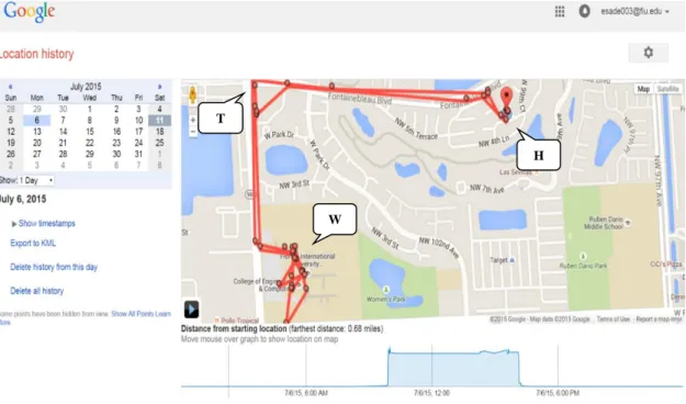
Figure 4-1 GLH Data Trace for a Sample Daily Travel ... 65
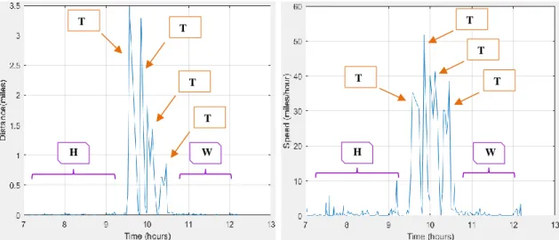
Figure 4-2 Sample Travel (a) Distance-Time (b) Speed-Time (c) 3D Space-time ... 66
Figure 4-3 Verification Trips (a) Distance-Time (b) Speed-Time (c) 3D Time-space .... 68
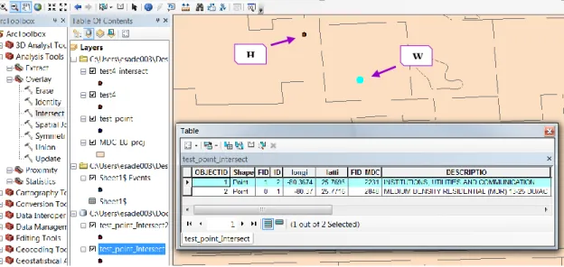
Figure 4-4 GIS Interface of a Sample Location Detection ... 71
Figure 4-5 GIS Interface of Home Detection ... 71
Figure 4-6 Locations Detection (a) Home Detection (b) Workplace Detection ... 72
Figure 4-6 Benchmarks of Data Verification Trip ... 73
Figure 5-2 Location of Home, Work and other of the Participant ... 77
Figure 5-3 Two-Dimensional Diagram of Longitude and Latitude ... 78
Figure 5-4 Two-Dimensional Diagram of Longitude and Time ... 78
Figure 5-5 Three-Dimensional Diagram of Longitude, Latitude, and Time ... 79
Figure 5-6 Schematic Example of Time Spent in Different Locations ... 80
Figure 5-7 Long-Distance Trip Frequency of Different Time of Day ... 81
Figure 5-8 Extra-Long Distance Trip Frequency of Different Times of Day ... 83
Figure 5-9 Long-Distance Trip Frequency of All Days of Week ... 84
Figure 5-10 Long-Distance Trip Frequency of Different Days of Week ... 85
Figure 5-11 Extra-Long Distance Trip Frequency of All Days of Week ... 86
ABBREVIATIONS AND ACRONYMS ATB Activity-Travel Behavior
CA Call Activities CDR Call Detail Records
FDOT Florida Department of Transportation GIS Geographic Information Systems GPS Global Positioning System GLH Google Location History IRB Institutional Review Board OD Origin Destination
INTRODUCTION
1.1.Background
In order to support transportation planning decisions, one must first have detailed travel information from people and households that can be used to understand travel behavior. Traditionally, these data were obtained from household travel surveys which suffered from low respondent rates, high respondent burden, and significant costs for survey implementation (Wolf et al., 2003; Pearson, 2004; Stopher and Greaves, 2007). Recent research has shown the promise of passively collected data to supplement/complement traditional household travel surveys. The term passively collected data means the data were collected without active engagement with the respondents, which could include GPS data, mobile phone network data, and etc.
In other words, as communication and information technologies advance, emerging data sources via passive collection methods have shown promises in helping transportation professionals better understand and map people’s movement through space and time. Traditional travel surveys are plagued by low respondent rates, high respondent burden, and significant costs for survey implementation (Wolf et al., 2003). Passively collected data, such as Global Positioning Systems (GPS) data, mobile network data, and cellphone GPS data, may have the ability to supplement and/or complement traditional household travel surveys and overcome existing issues.
A significant body of research has examined the use of GPS data and their capability to serve as an alternative to household travel surveys (Auld et al., 2009; Stopher et al., 2008; Hossan et al., 2017; Jin et al., 2014). Generally, the GPS device was fixed to
a participant’s vehicle or a participant was asked to carry the device daily (Boht and Maat, 2009; Pang et al., 2013; Vacca and Meloni, 2015; Dai et al., 2003. Although these studies indicated that the use of GPS could provide detailed travel trajectory data with sufficient level of accuracy, it had some limitations. The cost of purchasing the GPS units and administering the survey (mail the units to the participants and retrieve them back) could severely limit the size and length of this type of surveys. There is also certain level of respondent burden. For example, a participant could forget to charge the device or leave it at home which would render it useless.
Later studies started to explore the usage of cell phone data, particularly the Call Detail Record (CDR) data (Gonzalez et al., 2008). These data are produced and stored by the network providers whenever a subscriber uses a cellphone, such as making a call, sending a text, or browsing the internet. The CDR log records the time and location when that triggered; this location is calculated via triangulation. Due to the proliferation of cellular phones, a large sample of data could be obtained at minimum cost. Recent data indicated a penetration rate of 128% in developed, and 89% in developing countries (International Telecommunication Union, 2015). However, since the location information is indirectly measured, the CDR data tend to be less accurate than GPS data (Calabrese et al., 2013. These CDR data are measured via triangulation which means that during each usage activity, the signal of the phone is discovered by multiple cellular network towers. Therefore, the accuracy of this data can deteriorate for many reasons including a low number of available towers as well as tower switching to improve overall cellular network performance. In addition, the cellular phone must be in use to trigger recording, which
means no information is provided when the phone is inactive. This could leave significant gaps in the trajectory traces, which would compromise the use of the data.
In an effort to search for other data sources that overcome the current limitations, the goal of this thesis is to explore the potential of cellphone GPS data, which combines high accuracy with a high penetration rate and low respondent burden. These data can be easily obtained from cellular phones with an integrated GPS system. According to Wikipedia smartphone penetration was about 56% in the US in 2013, and is expected to increase every year (Wolf et al., 2001). Cellphone GPS data have an average accuracy of 31 feet, which holds great promises in travel pattern analysis with higher resolution rather than the CDR data with an accuracy of 164-984 feet (Lindsey et al., 2013).
1.2.Research Goal and Objectives
A quick review of the literature indicated that very few studies have focused on cellphone GPS data; most existing studies focused on GPS or CDR data. Nevertheless, these studies still provide valuable insights in terms of data processing algorithms and potential applications. A major challenge of passively collected data is that there is no participant input, so the researchers mainly rely on data mining techniques to derive useful information that describes mobility patterns.
The main goal of this study is to explore the potential of using smartphone data to collect transportation data to advance the understanding in mobility and travel behavior. The objectives of the study include: 1) explore the feasibility of the transportation data collection using the proposed method and develop algorithms and procedures to derive travel information from smartphones; and 2) identify applications in mobility and travel
behavior studies that could take advantage of these cell phone GPS data, which would not have been possible with conventional data collection methods. This research aims to demonstrate how accurate travel information can be collected and analyzed with lower cost using smartphone GPS data and what analysis applications can be made possible with this new data source. Moreover, the framework developed in this study can provide valuable insights for others who are interested in using cell phone data.
1.3.Dissertation Organization
This study is organized as follow: Chapter 1 introduces the study background, explains the problems, and states the goal and objectives.
Chapter 2 presents a literature review regarding different ways of collecting data such as CDR data, GPS, and mobile phone GPS data. In this chapter data processing methods and applications of the data are presented.
Chapter 3 elaborates on the survey design and data collection process for this study.. It describes the survey design and implementation process, including the questionnaire,, respondent recruitment, data collection, and results of the survey.
Chapter 4 describes the data processing algorithm to derive travel information from the GLH data, including trip ends identification, location identification, trip purpose identification, and validation of the results.
Chapter 5 presents further analysis of the travel behavior and mobility patterns based on the travel information derived, which demonstrates the advantages and potentials of incorporating smartphone GPS data into planning analysis.
Chapter 6 summarize the finding of this research and point out future research opportunities.
LITERATURE REVIEW
This chapter presents a detailed review of recent studies related to the applications of Global Positioning System (GPS) Data, Call Detail Records (CDR), and mobile phone GPS data; also known as passively collected data. Some of the applications of these data include trip end identification, trip purpose inference, traffic flow characteristics derivation, transportation mode estimation, location prediction, travel variability, Origin-Destination Matrix, Traffic Monitoring Traffic Monitoring, Rout Choice Model, and many more. All of these applications and other will be discussed throughout this section.
2.1.Passively Collected Data
The most important information contained within an individual’s travel data is coordinates and timestamps. These three sources which will be explained in this section are Mobile Network, Global Positioning System, and Mobile Phone GPS.
Some studies have been conducted a comprehensive review of trajectory data sources. The most recent and comprehensive of these was Yue et al. (2014). He constructed a review of studies related to travel behavior and categorized them by trajectory data types. In early studies data were mostly collected from household interviews or censuses. With these data researchers focused more on temporal, rather than spatial relationships.
Smart card, first used for automatic fare collection in public transportation, could be used in demand forecasting and travel demand modeling. However, one of the first concern in this field of research has been privacy. The actual and perceived ability of these data to accurately capture human mobility patterns has caused public concern to grow. Some the protection of this type of private data, with special attention to location. By
replacing a participant’s user name with a number, records became anonymous. Over the past decades, different types of trajectory data have begun to supplement conventional travel surveys as new collection methods have emerged. This renaissance of technology has also driven a new wave of travel behavior studies. “Big data” has brought opportunities and challenges for travel behavior studies. However, it seems that in future there will be more discoveries in trajectory-based travel behavior research based on “big data”.
2.1.1. Mobile Network Data
Mobile network data is a relatively new data source. Other attempts to improve travel surveys saw the incorporation of mobile network data, most commonly the Call Detail Records (CDR). The mobile network is comprised of a series of towers. The spacing and number of the towers, as well as signal strength, will directly affect the accuracy of the data. These data are recorded when a cellphone is transmitting Radiofrequency waves with cellular towers. Simply, data are only recorded when the phone is active, such as during a phone call or sending a message. Similar to GPS, the location of the cellphone is calculated based on the cellphone’s distance from surrounding towers. Using this method, it is possible to locate a phone within 50-300 meter accuracy (Federal Communication Commission, 2015).
In other word, this kind of data is recorded from cellphones, irrespective of the service provider. When a cellular device connects to the cellular network, the data is generated. A connection to the network can be established many ways but some of the most common include placing/receiving a call, sending/receiving a message, and connecting to
the internet. Typically, this source collects the device’s estimated location (latitude and longitude) and a timestamp for the connection.
As a cellphone moves, the signal will switch to the nearest and strongest towers’ signal. However, a phone does not need to move to switch towers. A phone can be observed to switch between towers, or oscillate, due to network policies regarding performance optimization or the proximity to competing cellular tower with equal strength. In respect to travel studies, oscillation can cause the data indicate false movements; a real movement could also be misinterpreted as the oscillation based on the repetitive nature of the movement.
A typical CDR dataset contains the caller ID, timestamp, duration of call or other activity, longitude, and latitude Other data, such as the call-receiver’s ID, may also be available. Due to privacy concerns, these ID’s are always anonymized and the formatting varies across carriers.
Due to the proliferation of cellular phones, a large sample of data can be obtained while greatly reducing the cost. Recent data indicated a penetration rate of 120% in developed, and 92% in developing countries (International Telecommunication Union, 2015). It should be stated that caution should be taken, as sampling mobile phone network could introduce bias or over represent participants with multiple phones. Not only is the scale of it enormous, this dataset also eliminates the respondent’s burden; most “respondents” are not even aware the data is being recorded. However, CDR data tend to be less accurate than GPS data. Since data are only recorded when the phones are in use, these data are less frequent and irregular. This could leave significant gaps in trajectory
traces, which complicates the application of the data. However, many studies have used these data successfully.
These data have been used for many applications including exploring mobility patterns and activity-travel behavior (ATB), estimating origin-destination (OD) matrices, developing procedures for generating mobile phone datasets, and location detection (Calabrese et al., 2013; Jarv et al., 2014; Iqbal et al., 2014; Chen et al., 2014; Cheng et al., 2012). Mobile network data has two types: cell phone user-based and cell-tower-based data. Cell phone user-based has anonymous user ID, cell tower ID, and information on phone call, data, time, and location. Cell-tower-based data has cell tower traffic information (Yue et al., 2014).
Calaberse et al. (2013) studied individual mobility patterns by using mobile network data. The authors suggested techniques to extract mobility information using cell phone tracing of millions of users within the Boston Metropolitan Area. The dataset included anonymous location estimations collected by AirSage from approximately one million cell phones.
The first step of the authors was to explore if individuals’ calling activities were frequent enough and produced sufficient data to monitor users’ movement. It was understood that this data would be less accurate than traditional GPS data. Additionally, network performance rules occasionally shift a caller to a further tower in order to maintain overall network performance. Due to this, it was noted that a user traveled several miles in just a few seconds. Although this did occur, it was not frequent enough to discount the entire dataset so the errors were rectified.
Following the error adjustments, trip lengths and home locations were estimated. The length of trips was calculated as the distance between consecutive network connections. Then, mobility measures were calculated and compared to existing mobility measures in order to check the validity of the data. Based on this, it was suggested that the data could serve as a representative source from which individual mobility could be calculated.
Jarv et al. (2013) studied activity-travel behavior (ATB) using call detail records (CDR), a form of mobile network data. Using CDR, their activity location and activity space for 12 months were examined. The object of the study was to reveal the variance in monthly behavior over a longer (twelve-month) study period and examine the factors that affect variability.
The files included information for all outgoing call activates (CA) of users in the network. The CDR data originated from EMT, an Estonian cellphone network operator, which had more than 500,000 active clients. The database had records of all outgoing CAs: text messages, calls, Internet connections, and data service initiated by the owner of the phone. The research focused on the people who were 20 to 64 years old and worked in Tallinn.
The results of the study of Jarv et al. (2013) showed that there was large monthly variance in the spatial distribution of activities. Moreover, ATB could be explained by individual (inter- and intrapersonal) factors and the impact of seasonality. It was understood seasonality had a marginal effect on the number of unique activity locations. Additionally, it was found that seasonality affects daily activities. One issue noted was that the frequency of phone usage had a significant impact on the results. It was concluded that
when using this type of data for human behavior research, the characteristics of individual phone use (calling, texting, or connecting to internet) should be taken into account.
Chen et al. (2014) developed a procedure for generating a simulated cellphone dataset which has the ground truth information. This study also sought to understand if a generated dataset could be representative of real-world mobility patterns. In the process of this, the researchers first had to identify activity locations from cellphone trace data; to do this, they were force to develop several items. In order to identify clusters, they developed a model-based clustering model which distinguished between activities and travel clusters; they also developed a logistic regression model that did this. To detect the different types of locations visited, they developed a set of behavior-based algorithms. This study defined trajectory as a set of time-stamped locations describing an individual’s movement in time, but other studies used drivers’ route choice on a highway network. The proposed simulated data (Dataset S) was comprised of two independent datasets: Dataset Ds and Dc. Ds contained household travel survey data and Dc which is a real-world cellphone data. In Dc, there were traces with corresponding time and location information and Ds contained unknown trajectories.
A total of 39,264 respondents were used in Ds; these came from the regional travel survey. Dc was comprised of trajectories with known time and location information. Based on these two sources, Dataset S was generated. It was shown that the simulated data’s distribution of the activity locations were more similar to the accurate than existing studies. For example, participants’ home and work were identified within 100m with 70% and 65% accuracy, respectively. It was concluded that the proposed methodology could illustrate
spatial and temporal patterns of mobility. The results indicated the possibility of using this generated dataset to replace traditional household travel surveys.
Cheng et al. (2012) analyzed activity patterns using cellular phone data in Shanghai, China. This study proposed a new method of extracting activities of individuals and the recognizing home and workplace Around 61 billion location data points from 324 individuals were collected over a two-month period. Home was identified as the location of a participant during the night (9:00 pm – 7:00 am), and work as the locations of a participant during the day (9:00 am – 12:00 pm and 2:00 pm – 5:00 pm). Next residents classified into three groups. Participants in Group 1 had their home identified but not work. Group 2 had both identified and the two are less than 5 Km apart. Similar to 2, group 3 had both locations identified but the two were far from each other.
The results showed that mobile network data can be used to analyze human activity patterns in space-time. It was also found that people that lived and work far apart, such as group 2 and 3, tended to have a time-varying activity area near the home or work. One of the major limitations of this study was the issue of privacy. The other was how the researchers defined home and work, which does not apply to every lifestyle or working schedule.
2.1.2. Global Positioning System Data
GPS devices communicate with a network, or constellations of around 30 satellites which orbit Earth at approximately 20,200 km. Although there are 30, a GPS device usually can only see about 12 due to the configuration of the satellites. Each satellite constantly
beams a signal towards Earth, but the position of a device is recorded every 1-4 seconds, depending on the device (United States of America Department of Defense, 2015).
To identify the location of a GPS device, the distance between a satellite and the device is calculated. Connecting to two satellites provides the longitude and latitude. Incorporating a third satellite facilitates the calculation of the altitude; any additional satellites can increase the accuracy. Today, GPS has a vertical accuracy of five meters (or better) and horizontal accuracy of three meters (or better) 95% of the time (United States of America Department of Defense, 2015). The accuracy will be highest when the device is in clear view of the satellites (such as in an open field) and will suffer when obstructed the lowest while the (between high-rise buildings or in a tunnel).
GPS datasets always contain a timestamp, longitude, latitude, altitude, and speed for each data point. It is not uncommon to see the heading and a measure of accuracy such as the number of satellites in communication with the GPS device, included in the dataset (Lindsey et al., 2013).
In the majority of studies, a GPS device was fixed to the vehicle or the participant was asked to carry the device daily. Although most studies related to GPS devices indicated that travel trajectories with a high level of accuracy can be provided, there are some limitations. The first issue is the monetary limitation. The cost of purchasing the devices and administering the survey (mailing and retrieving the units to participants) can severely limit the scale and duration of this type of survey. Moreover, there is certain level of respondent burden. For instance, a participant may forget to charge the device or leave it at home which would render it useless (Stopher et al., 2008). This source is always more accurate that mobile network data (Calabrese et al., 2013).
Studies which need very accurate position data tend rely on GPS data. For instance, studies that focused on transportation mode detection and developing mobility models for walking have been accomplished with GPS data (Zheng et al., 2008; Lee at al., 2009). Its accuracy also lends it the ability to supplement previous data collection methods, specifically surveys. Studies, such as Yue et al., 2014, proved that GPS data could potentially replace traditional diaries.
Zheng et al. (2008) studied the mobility based on GPS data of people in China. The purpose of the study was to propose an approach to predict participants’ transportation mode. The authors collected the data from 65 people over ten months. Features such as heading change rate (HCR), stop rate (SR), and velocity change rate (VCR) were identified. A graph-based post-processing algorithm was proposed to further improve the predictions. The approach had two parts, online inference and offline learning. It was observed that employing new features caused an eight percent improvement, over previous studies, of mode inference accuracy.
Lee et al. (2009) studied the mobility models for walking in South Korea. The main purpose of the research was to present a new mobility model which can produce trajectories for the walking mode. The authors presented the SLAW (Self-similar Least Action Walk) model. The model was generated for applications where people share common interests or are in a single community, such as a university. Developing SLAW relied heavily on GPS recorded human walk trajectories, including 226 daily traces collected in five different outdoor sites from 101 participants. It was concluded that SLAW could generate the unique performance features of different mobile network routing protocols; people within a single community or with similar interest had certain mobility patterns.
2.1.3. Mobile Phone GPS Data
The most recent efforts to improve travel surveys were made possible with the advent of cellphone GPS, or assisted GPS, data. This technology represents a merging of mobile phone network and traditional GPS data. Mobile phone apps have been used in previous transportation studies (Sunio and Schmocker, 2017; Massahi et al., 2016). Similar to mobile network data, cellphone GPS data have the potential for large scale applications and a reduced, but not eliminated, respondent burden. Due to the cellphone GPS chip’s energy demand, recording data can reduce battery life. Also, depending on the source, retrieving this information may place a burden on the respondent; this sample could introduce bias. As a hybrid between the previous sources, cellphone GPS data have an accuracy level near that of GPS data (9 meters (Lindsey et al., 2013)) while maintaining the high penetration rate, low cost, and minimal burden similar to the CDR data.
A cellphones position is calculated in nearly the same manner as GPS and mobile network, via triangulation. Data points in this dataset can be recorded via Wi-Fi, GPS satellite, or mobile network; certain phones allow user control over how the data is recorded in an effort to conserve power. It is possible to track the phone even when it is not being used, and it can be tracked without the cellphone signal if the phone is in-view of the satellites.
With the advances of smartphone technology, GPS-like data can be collected from a smartphone rather than a GPS device. For instance, travel behavior characteristics such as the number of activity locations visited and size of individuals’ activity space (Ythier et al. 2013), as well as transportation mode (Ansari and Golroo, 2015) can be studied. It was also demonstrated that this new technology can measure position and velocity of vehicles
and used in applications like the traffic monitoring (Herrera et al., 2010). Additionally, using GPS-enabled smartphone, the location of the users can be identified by 100% accuracy. GPS uses so much battery power, however, with new charging technologies, such as wireless chargers, it is not a significant problem to use GPS of smartphones (Hariri et al., 2016; Hariri et al., 2017).
Ythier et al. (2013) studied the influence of social contacts on travel behavior. The purpose of the research was to exploit individual-level data from smartphones to investigate the influence of calling/texting on spatial movement and study the effect of social contact/communication patterns on travel behavior. The authors described how variables can be processed from the data and estimated results using regression analysis. Three concepts were used in the study. Travel behavior which could be explained as travel intensity, which is the number of activity locations visited, and size of individual’s activity space, which is the area that most activity of the traveler spends time. Five variables were used as travel behavior characteristics: number of trips, number of activity locations, number of occasional activates, average distance per trip, and maximum distance traveled between home and an activity location.
The study’s sample was comprised on 111 participants in Switzerland over three months. In this study, participants carried a N95 mobile phone. Using GPS, longitude, latitude, and altitude with time step of 10 seconds were accessible. However, participants were allowed to turn on/off the device to save battery life which made the data incomplete. Moreover, information of calls, such as duration of outgoing, incoming, and missed calls, as well as outgoing and incoming of text messages, were gathered. It was proved that mobile phone data could be used for understanding the travel behavior, even once they
were collected for billing purpose. It was concluded that the travelers were influenced by their social context. Moreover, the socio-economic characteristics influenced the travel intensity and travel behavior.
Ansari et al. (2015) studied transportation mode choices from a smartphone GPS dataset. The main goal of the study was to identify transportation modes used by the participants via machine learning method. Another purpose was to define attributes for mode classification and determine influential factors. An application was installed on participants’ mobile phone to record their data (GPS track). The sample was comprised of traces for 25 males and 10 females and was collected over two week between 6:00 AM until 9:00 PM. All participants were asked to keep a record of their modes to complement the data. The model could classified transportation modes with around 96% accuracy, which was higher than previous studies.
Herrera et al. (2010) studied a traffic monitoring system based on GPS-enabled smartphones. The study was a proof of concept of a system which was able to measure position and velocity accurately. This presented a field experiment nicknamed Mobile Century which includes 100 vehicle that carried a GPS-enable Nokia N95 phone driving loops on a 10-mile stretch in California for 8 hours. Data were collected using Virtual Trip Lines (VTLs). Virtual Trip lines are geographical markers stored in the handset that probabilistically trigger position and speed updates once the headset crosses them. It was possible to compare the velocity measurements collected by both loop detector and VTLs as well as the computation of penetration rate achieved during the day.
As it was very difficult to collect ground truth velocity information, loop detector velocities were used for comparisons against travel times in order to assess the accuracy of
the data. It was understood that VTL measurements exhibit more variability than loop detector measurements, so the study used the 5-min aggregation method. Based on observations, it was suggested that a 2-3% penetration for these mobile devices would be enough to have an accurate measurement of the velocity of the traffic flow.
The field operational test in the initial phase of the development, called the Mobile Millennium, consisted of the free distribution of traffic software such as the software presented in this paper to regular commuters, and the collection of travel time during the months, and would cover North California in its initial phase. The system had mobile sensors to detect the GPS-enable phones and static (loop detectors) which were expected to provide a more accurate estimation of traffic. Aside from the accuracy of data collection, another advantage of the proposed traffic monitoring system is that the system needs very little installation and maintenance cost. Due to this, the method could potentially be used in developing countries where there is a lack of the resources and monitoring infrastructures.
Yin et al. (2014) evaluated the accuracy of vehicle positioning using GPS-enabled smartphones. Thy intended to compare the results of different methodologies of identifying vehicles’ location. The four data sources which the authors used were professional GPS handset, GPS-enable smartphone, cellular network positioning, and GPS-enable smartphone with Geo-fence. In the first scenario GPS-enabled smartphone was compared to a professional GPS handset, Juno. Second scenario, compared cellular network estimated handover points. In the third scenario, GPS-enable smartphone was compared with Juno. The data were collected from 1:00 PM to 4:00 PM on vehicles commuting on a road in Alberta with twelve Geo-fences. Analyzing the results of the three scenarios, it was
understood that GPS-enabled smartphone could identify the location of user by 100% accuracy; cellular positioning system was lower. Results of a combination of Geo-fence and smartphone positioning was the most accurate.
2.1.4. Google Location History Data
Another way to collect the data of smartphone owners is through Google Location History (GLH). Google’s location service uses Wi-Fi, and other signals, to determine location more accurately and often with lower power usage comparing to GPS. GPS helps provide the device with a precise location, hence, it can be used for turn-by-turn navigation and routing. However, it consumes a ton of battery life. The location service circumvents this problem by using signals that the device is usually using in the first location. It hones in on cell sites and Wi-Fi signals to locate the device accurately.
Cellphone GPS data’s recording frequency varies based on movement, with less data records when the phone is still. Using Google Location History (GLH) data as an example, while the cellphone was in movement, data were usually recorded every 30-60 seconds; while the phone was still, the recording rate increased to over 1 minute and rarely exceeded 5 minutes. Due to the varying recording interval, it is possible to record greater than 1,000 points per day. GLH data can be accessed as a KML or JSON file. Both files provide information on the timestamp, longitude, and latitude.
The locating method by cell phone is adjustable. For instance, for Android system, choosing the second Location option on the setup screen, which is Power saving, let the smart phone even scan Wi-Fi signals when Wi-Fi is off, and it can be done with the minimal hit to the battery. Every single point on the map indicate where Google used Wi-Fi
Positioning System (WPS) to locate the device. Each time the smartphone is within range of a Wi-Fi access point, it would send its MAC address and SSID to Google’s servers. Using GPS (when available) and cell ID data, the Wi-Fi access point can be located, and based on the collected data the history on the map is created (How-To Geek, 2015).
Google operates many location-based services on smartphones. For these services to work best, they need access to the mobile phone owner’s location data. Moreover, Google Maps may store places the traveler has been recently and use them to show more relevant search results. Google does not share the individual’s location history with others or marketers without individual’s permission (Androidcentral, 2015).
2.2.Data Processing
This section discusses an overview of the data processing methods done to the aforementioned data. As indicated by the literature, data processing involves pre-processing, trip end identification, trip purpose identification, and trip mode detection. The main intention of this section is to understand the scope and level of efforts required to use this data.
The first step is pre-processing, usually accomplished through criterion-based data elimination. Speed and location of data points were noted as commonly used criterion to eliminate data. The most common criteria was to remove the data points with unreasonably high speeds (Huntsinger and Ward, 2015; Wang et al., 2013; Sharman and Roorda, 2010). The capabilities of Geographical Information Systems tools (GIS) were also implemented. In one case, the data outside of the study area or outside the desired zones were removed (Zanjani et al., 2015). Moreover, considering time or distance between consecutive data
points has proven to be effective (Berlingerio et al., 2014). In some cases pre-processing involves the removal of trajectories when there was insufficient data (Stopher et al., 2008). Although labor intensive, manual checking was also noted.
At the disaggregate level, considering the distance or time between consecutive data points has proven to be effective (Zanjani et al, 2015). Sometimes pre-processing also involves the removal of data where insufficient data points can be obtained (Bohte and Maat, 2009); although labor intensive, manual checking may also be helpful.
2.2.1. Trip Ends Identification
Various attributes have been used in previous studies to identify trip ends. Many studies used time-constrained rules, however, it tended to work best when the dataset is complete (no signal loss). Trip ends could also be detected when the speed is zero or very low (Nour et al., 2015). Other researchers used the “dwell time” or the amount of time spent at a specific location. This duration was calculated as the difference between departure and arrival time (Berlingerio et al., 2014; Wang et al., 2015; Sadeghavziri et al. 2016). It was also noted that many of these studies used conditional statements whereby both conditions needed to be satisfied to identify a trip end. Some studies also used GIS to help identify trip ends. These cases used data clustering, geo-referencing, and referred to the first/last recorded point of a trajectory (Stopher at al., 2008; Zanjani et al., 2015; Lu et al., 2010).
Some researchers defined activity locations based on duration, frequency, and time-of-day (Fang et al., 2014), as well as point density or other clustering methods in which points were assigned to a cluster based on the relative distance (Zheng et al., 2008). Chen
et al. (2014) showed the potential for the application of a model-based clustering algorithm to identify clusters which were then divided into trip end clusters and travel clustering.
Many studies also used the capabilities of GIS to help identify trip ends, including data clustering (Bohte and Matt, 2009), geo-referencing (Sharman and Roorda, 2010), and retrieving of the first and last recorded points in a trajectory (Lu et al., 2010).
During instances when there is no signal, many studies used the time between consecutive points as a proxy dwell time to detect the trip end. For instance, it is possible to assume that if the location of point A and point B does not change significantly over a time interval when no signal is available, the location is a single trip end. Nonetheless, if the distance between the two points changes significantly during the time interval, most likely that missing data is best represented by a trip rather than a trip end (Schussler and Axhausen, 2009).
Some researchers used GIS (Jarv et al., 2014) and others used criteria to detect Home and Work. For instance, one study (Calabrese et al., 2013) divided the study area into a grid of 500 m by 500 m cells in order to help with home/work locations. The number of nights (6:00 PM - 8:00 AM) spent in each cell was tabulated and the cell with the highest frequency was identified as home.
2.2.2. Trip Purpose Identification
In most studies, trip purpose identification was the most difficult step. Some researchers used GIS to facilitate this process and incorporated the land use patterns. Generally, trip purpose identification was accomplished by three main methods: criterion-based, probabilistic, and machine learning methods.
Generally, the criterion-based method was applied with land use patterns (Bohte et al., 2009; Schonfelder et al., 2003; Pereira et al., 2013). General trip end rules, such as assigning a purpose as shopping if a trip end was located near a known shopping mall, were also used (Wang et al., 2010; Berlingerio et al., 2014; Fang et al., 2014). However, many time, these studies relied on information provided by the participants. Another method was to consider time-of-day and duration were after proximity rules were applied (Cheng et al., 2012; Wang et al., 2013). Some researchers applied a probabilistic approach. For instance, Chen et al. (2014) employed a Multinomial Logit Model in high density areas and a single deterministic matching method in low density areas (Bohte et al., 2009). Another explored the use of Nested Multinomial Logit Models (Wolf et al., 2014, Axhausen et al., 2003) to determine the purpose of the trip based on probabilistic calculations related to the trip distance.
Machine learning, specifically Decision Trees (Ansari and Golroo, 2015; Bohte and Maat, 2009), were employed to detect the purposes of trips. Compared to the first method, probabilistic and machine learning methods were used less due to their complexities. Of all the procedures, trip purpose identification is the area which has the most room for improvement.
2.2.3. Trip Mode Identification
There are different methods which can be used to detect the travel mode, but the most common criteria is speed. Average and maximum speed (Bohte and Maat, 2009; Sadeghvaziri et al., 2016; Alluri et al., 2017), the statistical mode of speed (Nour et al., 2015), a range of average and maximum speeds (Bohte et al., 2008), and the average
acceleration for each mode (Zanjani et al., 2015; Lee et al., 2009) have been applied successfully and applicable to most situation in order to detect the mode of travel.
Another method is using GIS to consider the built environment’s characteristics (Hosseinlou et al., 2012). For instance, pedestrians can only walk on links which are accessible to pedestrians. In addition, other researchers used buffer zone in GIS. For instance, Bohte et al. (2009) created buffer zones around rail stations and bus stops. Being near a known point, or inside a buffer zone, allowed researchers to identify rail and bus modes.
There are other methods for travel mode detection. Some researchers developed a probability matrix (Huntsinger and Ward, 2015; Nitshe et al., 2012; Rojas et al., 2016; Abdi Kordan et al., 2014; Sadeghvaziri et al., 2016; Nitshe et al., 2014), and other researchers deployed fuzzy logic methods (Schüssler and Axhausen, 2008). Although these method were effective at identifying walking and cycling modes, they struggle to differentiate between motorized modes (Wolf et al., 2014).
As machine learning method has a high level of accuracy, it is an emerging approach for travel mode detection (Stenneth et al., 2012; Hosseinlou et al., 2012). In this area some common methods are Decision Tree (Reddy et al., 2008), Support Vector Machine (Pereira et al., 2013; Jahangiri and Rakha, 2014; Zhang et al, 2011), Baysian Network (Moiseeva et al., 2010), Random Forest (Ansari and Golroo, 2015), and Multi-layer Perceptron Neural Network (Das et al., 2015; Gonzalez et al, 2010).
Ansari et al. (2015) detected the travel mode using a machine learning method which was fed smartphone GPS data; 35 participants over 14 days. They also studied attributes for mode classification and determined influential factors. There are two main
methods in mining data and to find the pattern of travels based on GPS traces: procedural and machine learning. In procedural method, based on logical assumptions, the mode of the travelers can be identify. For instance, availability of bicycle at home and low speed of the traveler are hints to interfere that the passenger used his/her bicycle. Machine learning method is very suitable to analyze data through complex approaches and it has been used to identify transportation mode of travelers. As machine learning methods could be used to forecast with high accuracy, it was used in this study. Speed, distance, acceleration, and heading differences were considered as the four main attributes to distinguish different modes. This study also considered new attributes: acceleration, acceleration changes, and heading changes. These attributes were defined based on some logical rules. For instance, acceleration and changes in acceleration would not be very large when walking. Also, walking allows greater freedom to change direction, or heading, than a motorized vehicle. The model was able to detect the travel mode with 96% accuracy. It was concluded that speed was the most dominant attribute in the process of transportation modes classification which was consistent with previous studies.
2.2.4. Location Identification
Chen et al. (2014) developed a set of behavior-based algorithms to identify locations types. They observed three main patterns of cell phone usage that helped identifying activity types at locations. First, as people spend more time at work and home than other places, more sightings were generated at work and home locations. Second, as most individuals depart from home to work at similar times, stay at work for a set period, and go home at similar time, these points could serve as a basis for comparison. Third,
sightings indicated distinct time frames. Most sightings generated at work were during daytime hours and most sightings generated at home were during evening because of individuals natural biological clock is to be at work during daytime hours and at home during evening. Moreover, Cheng et al. (2012) considered the places where the users spent time at night (9:00 PM-7:00 AM) as home and the places where they spent time during the day (9:00 AM-12:00 AM and 2:00 PM-5:00 PM) as work. It is worth mentioning that researchers commonly used timestamps in Unix format; this displays time as a digit which can be easily read by computer and easily converted to be read by humans. For instance, Feb-22-2015 at 13:20:00 is 1424568000 in Unix format. During two months, location traces of 774 individuals were gathered and then analyzed.
Few researchers studied the location prediction accuracy regarding the length of location history. For instance, the purpose of the study of Wang et al. (2014) was to investigate the relation between the length of location history and prediction accuracy for subpopulation which has different level of uncertainty in their trajectories. This study applied entropy S as an indicator of the amount of information input in the predictor. An individual’s trajectory with S = 3 means (2S=23=8) that an individual could be in 1 of 8 possible locations. Entropy was measured based on the temporal-uncorrected entropy with the Equation (1):
𝑆𝑖𝑢𝑛𝑐 = − ∑𝑁𝑖𝑗=1𝑃𝑖(𝑗) log2𝑃𝑖(𝑗) (1)
In this formula Pi(j) is the historical probability that location j was visited by the individual i. Mobile data set which was used in this research was obtained from mobile
phone positioning data. As soon as the mobile phone communicated with the tower, a unique ID number, time, and location was generated. It was found that the level of uncertainty in trajectories was a function of the amount of input information required for correct prediction of the location and low level of uncertainty resulted in a high level of predictability accuracy. For instance, given 100 historical location, for people with low and high level of uncertainty, prediction accuracy would be 80% and 50%, respectively. On the other hand, if a prediction accuracy level over 60% was required, just 10 historical location is enough.
This study found that based on a desired accuracy level, the size of location history could be determined. This implies that limited amounts of input is required for travelers who have a low level of uncertainty in their trajectory. Therefore, it is possible to discard data without compromising the model’s prediction accuracy. Moreover, it was shown that for individuals who had high level of uncertainty trajectory, very long location history did not necessarily provide increased accuracy predictions. For example, for individuals who had highest level of uncertainty in their trajectories, accuracy of prediction stabilized between 50% and 60%.
2.3.Data Applications
This section discusses the transportation applications that can be obtained from these data sources.
2.3.1. Traffic Flow Characteristics
Having accurate data, the different flow can characteristics can be obtained. The three main characteristics that can be obtained with accuracy are travel time, travel speed,
and traffic volume (Bar-Gera, 2007; Liu et al., 2008; Massahi et al., 2016; Caseres et al., 2012; Massahi et al., 2017). For instance, Bar-Gera (2007) aimed to examine the performance of a new operational system to measure travel time and traffic speeds from cellular phone service provider data. They compared cellular measurements with those obtained from magnetic loop detectors. Their case study was a 14 km freeway with ten interchanges over two months. The cellular phone-based system recorded observations for about 2% of the total traffic from 10:00 AM to 2:00 PM, and generated 440331 (63%) travel time estimates for 27 sections. Travel times converted to an average section speed simply as the ratio of road length to estimated travel time. The main finding of their study was that there was a good match the between two measurement methods and that the cellular phone-based system could be useful.
Liu et al. (2008) aimed to study travel time and speed using cell phone data. Traditionally, traffic condition could be measured using loop detectors. However, new technologies have become available recently that can assess traffic conditions by tracking vehicle trajectories and travel times. Among new technologies, smartphones have received strong interest from the transportation field. AirSage, Inc., has constructed a proprietary system that can track cellphone movement in Minnesota and deliver travel times for most of the urban roads, including both signalized arterial and limited access freeways. The performance of the system was evaluated, including system’s accuracy during the peak hours over a 16-day period. Speeds were calculated by dividing travel times (for AirSage’s reported and the observed conditions) by the ground truth segment length and converted to miles per hour. The technology produced results with varied accuracies.
Another application of these data is obtaining the traffic volume. Volume is commonly collected by using on-road (fixed) sensors such as cameras and inductive loops. The installation of fixed sensors to cover all roads is impractical, and not economically feasible. Due to this, they are only installed on subset of links. Cellular systems provide alternative methods to detect phones in motion without the cost and coverage limitations related to those infrastructure-based solutions. Caceres et al. (2012) proposed a set of models that could infer the number of vehicles moving from one cell to another by means of anonymous call data of phones. A set of inter-cell boundaries with different traffic background and characteristics were selected for the field test. The results showed that reasonable estimates were achieved by comparison with volume measurements collected by detectors that were located in the same area.
2.3.2. Origin-Destination Matrix
There are many studies which were able to apply the available data to produce OD table. It was proved that with both GPS (Thakur et al., 2014) and CDR (Wang et al., 2013) data, trips can be reproduced accurately. However, most studies used CDR data to infer trips and then estimate large scale OD matrices (Colak et al., 2015; Iqbal et al., 2014; Sharman and Roorda, 2010; Schussler and Axhausen, 2009). Later, Zanjani et al. (2015) were able to estimate Florida’s statewide OD truck flows.
By incorporating time-of-day, another study found that it was possible to create OD sample characteristics, mobile OD flow distributions, directional patterns, and spatial analysis; flow analysis for each OD pair was also conducted (Li, 2015). Moreover, to
capture more detailed information, Rokib et al. (2015) used similar CDR data in combination with Foursquare check-in data to reproduce OD matrices.
Iqbal et al. (2014) developed origin-destination matrices using cell phone call data. The authors proposed a methodology for developing OD matrices and traffic counts, using cell phone CDR. The patterns of trips were extracted from cell phone and ground traffic scenario was derived from traffic counts. First, CDR, which had time stamped tower location with caller IDs, were analyzed and then trips were used for generating tower-to-tower OD matrices. Then these are associated with corresponding nodes of the traffic network and converted to node-to-node transit OD matrices. The CDR data was collected from Grameenphone Ltd, and it was consisted of call from 6.9 million users. A total of 13 locations of Dhaka were chosen and video data of them were collected over three days. The study was done in central part of capital of Bangladesh, Dhaka, and CDR from 2.87 million user over one month and traffic data from 13 key locations over three days were used. As CDR is recorded for billing purposes by cell phone companies, this way method is more economic than traditional ways which were based on household surveys. The ODs applied to simulate the traffic between 9:00-12:00 in MITSIMLab, then simulation’s results were compared against the observed counts form 4 other locations. As a limitation, the transferability of the models in MITSIMLab was not tested in detail and just key constants of the model were updated to better match the patterns of traffic of Dhaka. The method is effective for places where land use pattern is heterogeneous and there is a limitation of traditional data sources.
Many studies focus on route choices of individuals. For instance, Levinson et al. (2013) investigated the rout which driver choose for a period of 15 days using GPS. The results showed that the participants did not have a single dominate route.
In another study, which was also based on GPS data, the authors identified four types of heterogeneous driver learning and choice evolution patterns (Tawfik and Rakha, 2012). This study had three main findings. First, the observed route choice percentages varied from those derived by using stochastic user equilibrium expectations, but approached specific values. Second, the study identified four types of heterogeneous driver learning and choice evolution patterns. Third, driver and choice situation variables can predict the identified learning patterns.
Dhakar et al. used combination of GPS and GIS data to develop models for rout choice. The results showed statistically significant and reasonable effects of free-flow travel time, intersections, right turns, left turns, and circuity on the attractiveness of different route alternatives (Dakhar and Srimivasan, 2014).
Casello and Udyukov (2014) also used GPS data to study effective path parameters. They used logit models to determine the relative importance of four statistically significant path parameters including grad, auto speed, length, and the presence of bike lanes. It was concluded that possibility of generating a relative robust path and mode model which can be included into multimodal travel forecasting models.
In another study, Spissu et al. (2011) used GPS data explore the route choice models. They successfully, converted GPS data into routs in order to characterize route choice variability and compare the least-cost rout to the actual rout. The study analyzed a GPS-based dataset of 679 routes, collected by a personal probe system called the activity
locator over two weeks for a sample of 12 students from University of Cagliari in Italy. It was shown that the higher levels of intra-individual variability were found for discretionary trips. Moreover, higher levels of inter-individual variability, as well as greater deviation from minimum-cost routs, are associated with study and work trips.
2.3.4. Daily Variability
Another common application encountered in the literature review was daily variability (Huff anf Hanson, 1988; Hanson et al., 1982). Variability in travel behavior has received little attention in the literature review. The main reason is that most data sets used for analyzing and modeling urban travel comparison information for just a single day for each sampled individual and therefore preclude examination of variability (Pas and Koppleman, 1987; Baqersad et al., 2017). Having multiple days’ data available, still the variability in travel pattern is not obvious. Although individuals’ travels have a spatial nature, most studies focused on non-spatial aspects, such as daily travel distance, number of daily trip, and daily travel time (Wang et al., 2017). Not having a comprehensive knowledge on variability in spatial dimensions, such as activity lactations, lead to a potential gap in current thinking on the relationship between activity-travel behavior and the consumption of urban space (Buling et al., 2008). For example, a traveler may have a same number of trips on two days, however, to completely different sets of activity locations.
Location variability characterize travelers’ activity location choice behavior and activity location choice has been proved to be affected by time of day (Kitamure er al., 1998; Baqersad et al., 2017). Therefore, it is important to know whether the travelers’
location variability depends on the time of the day. Time-of-day dependence of location variability is relevant to the concept level of fixity. It is a measure reflecting the extent to which activities are constrained in space. Obviously, those kind of activities which have higher level of fixity are more difficult to relocate and reschedule. Activities with the highest level of fixity are compulsory activities such as school and work (Kitamura and Van, 1987; Shafieifar et al., 2017). Among all activities with different level of fixity that an individual performed, the individuals’ locations during time between activities with higher level of fixity have less variability.
Generally, for evaluating location variability, the frequency of repeat visited to activity locations is measured. One study (Kitamura and Van, 1987) studied the individuals’ activity locations and the results showed that the trips related to two to four most visited locations accounted for more than 70% of all trips. Based on the result of another study (Buliung et al., 2008), individuals did 72% of all their activities at repeated locations and 28% were carried out ate location occurring only once during one-week period. In another study, Song et al. (2010) explored the fraction of time a mobile phone owners spent at their top-visited locations. It was found that individuals spent around 60% of their time at their top two locations. Lu et al. (2013) studied the predictability in human mobility and found that those who visited more than ten locations, spent around 75% of their time at the top two locations, meanwhile, this percentage is about 95% for those who only visited four distinct locations. Therefore, it can be concluded that the individuals’ locations choices presented a significant amount of repetition which is same as conclusion of Schonfelder (2001).