http://siba-ese.unisalento.it/index.php/ejasa/index
e-ISSN: 2070-5948
DOI: 10.1285/i20705948v9n1p122
A comparison of missing data handling methods in linear structural relationship model: evidence from BDHS2007 data
By Mamun et al.
Published: 26 April 2016
This work is copyrighted by Universit`a del Salento, and is licensed un-der aCreative Commons Attribuzione - Non commerciale - Non opere derivate 3.0 Italia License.
For more information see:
DOI: 10.1285/i20705948v9n1p122
A comparison of missing data handling
methods in linear structural relationship
model: evidence from BDHS2007 data
A.S.M.A. Mamun
a, Y. Z. Zubairi
b, A. G. Hussin
c, and S. Rana
∗daDepartment of Statistics, University of Rajshahi, Rajshahi-6205,Bangladesh
bMathematics Division, Centre for Foundation Studies in Science,University of Malaya, Kuala
Lumpur, Malaysia
cFaculty of Defence Science and Technology,National Defence University of Malaysia, Kuala
Lumpur, Malaysia
dDepartment of Mathematics / Institute for Mathematical Research, Universiti Putra Malaysia,
43400 UPM Serdang, Selangor, Malaysia
Published: 26 April 2016
Missing observations in dependent variable is a common feature in survey research. A number of techniques have been developed to impute missing data. In this article, we have evaluated the performance of several impu-tation methods namely mean-before method, mean-before-after method and expectation-maximization algorithm in linear structural relationship model. On the basis of mean absolute error and root mean square error for both simulated and real data sets, we have shown that expectation-maximization algorithm is the most effective method than the other two imputation meth-ods to analyze the missing data in linear structural relationship model.
keywords: Errors-in-variable model, Imputation method,
Expectation-maximization algorithm, Performance indicator, Demographic health survey.
1 Introduction
Missing data are a part of almost all research and it has a negative influence on the analysis, such as information loss, as a result, a loss of efficiency, loss of unbiasedness of
∗
Corresponding author: sohel [email protected]
c
Universit`a del Salento ISSN: 2070-5948
estimated parameters and loss of power. There are several reasons why the data may be missing. They may be missing because of equipment malfunctioned, the data were not entered correctly, sometimes respondent skip questions out of fear of getting in trouble or a subject may be removed from a trial if his/her condition is not controlled sufficiently well. Based on the different reasons, missing data can be classified as missing completely at random (MCAR), missing at random (MAR), and non-ignorable (NI) missing values (Littlel and Rubin, 2002) and these classifications influence the optimal strategy for working with missing values.
Several studies (Hippel, 2004; Winkler and McCarthy, 2005; Littlel and Rubin, 2002) have been conducted on how to deal the data set with missing values. Imputation methods are one of the most widely used technique to solve incomplete data problem (Littlel and Rubin, 2002). Therefore, this study stresses on several imputation methods to determine the best methods to replace missing data.
From a complete data set, incomplete data sets need to be generated in order to com-pare different methods. Many researchers (Junninen et al., 2004; Twisk and Vente, 2001; Norazian et al., 2008) generated randomly simulated missing data patterns for evaluating different methods in different types of data sets, as for example, air quality data sets and longitudinal studies. Perneger and Burnand (2005) applied simple imputation algorithm to reduced missing data in SF-12 health surveys. Moreover, Kofmanhttp (2000) applied the imputation method for incomplete dependent variables in the financial data set.
In this article, we generate different missing data patterns in dependent variable and apply three imputation methods on Bangladesh Demographic and Health Survey 2007 data (NIPORT et al., 2009) namely the mean-before, mean-before-after and expectation-maximization (EM) algorithm for the parameters of linear structural relationship model (LSRM) assuming the ratio of error variance is known. The performance of imputation methods is measured using mean absolute error and root mean square error. We orga-nize this article as follows: Section 2 gives materials and methods which includes the brief description of the estimation of parameters in LSRM, mean imputation techniques, expectation-maximization algorithm, performance indicators, simulation studies and de-scription of the data BDHS 2007 data. Section 3 envelops the results and discussion of the study. Finally, in Section 4, a conclusion is given.
2 Materials and Methods
2.1 Estimation of parameters in LSRM
Consider the following circumstances
Y =α+βX (1)
where, there exists a linear relationship between the random variables X (heights) and (weights) and suppose that they are measured without error.
However,in reality, these two variables X and Y are not observed directly, i.e., they are measured subject to error. Ifδi andi are the two respective errors in measuringXi
and Yi , then we can write xi =Xi+δi and yi =Yi+i , where the error terms δi and
i are normally distributed having zero mean and varianceσ2δ andσ2 ,respectively. This
reveals that the variances of error are not dependent oniand so independent of the level of X and Y, which assumed homoscedasticity. There are some assumptions that have been described in the literature for obtaining the X values. For example,Kendall and Stuart (1973) described the structural model consideringXi as normal distribution with
mean µand variance σX2. In LSRM, the errors are assumed to be normal, the bivariate normal distribution ofxi and yi , is then
xi yi ! ∼N " µ α+βµ # , " σX2 +σδ2 βσ2X βσX2 β2σ2X+σ2 #! (2)
Kendall and Stuart (1973) have shown that there are five equations with six unknown (µ, α, β, σX2, σ2δ, σ2) , hence an additional assumption is required for the unique and consistent solutions of the parameters of the model (1). In particular, Hood et al. (1999) discuss in detail estimation procedure to estimate the model (1) under various assumptions. However, for the case when the ratio of error variance λ= σ2
σ2
δ
is assumed to be known, the Maximum Likelihood Estimate (MLE) for the parameters are given by
ˆ µ= ¯x (3) ˆ α= ¯y+ ˆβx¯ (4) ˆ β = (Sy2−λSx2) +q(S2 y −λSx2)2+ 4λSxy2 2Sxy (5) ˆ σX2 = Sxy( ˆβ 2S2 y + 2λβSˆ xy +λ2Sx2) ( ˆβ2+λ)( ˆβS2 y+λSxy) (6) ˆ σδ2= ( ˆβS 2 x−Sxy)( ˆβ2Sy2+ 2λβSˆ xy+λ2Sx2) ( ˆβ2+λ)( ˆβS2 y+λSxy) (7) where,S2
x , Sy2 and Sxy are defined as Sx2 = n1 P
(xi −x¯)2, Sy2 = 1n P
(yi −y¯)2 and
Sxy = n1P(xi−x¯)P(yi−y¯) ,respectively.
Recently, Carpita and Ciavolino (2015) proposed generalized maximum entropy (GME) estimator for a simple linear measurement error model with a composite indicator. Fur-ther, they (Carpita and Ciavolino, 2016) developed GME estimator for the regression model with a composite indicator as explanatory variable.
2.2 Mean Imputation Techniques
Let us consider n observations x1,x2,...,xn of which m values are missing denoted by
x∗1,x∗2,...,x∗n.Thus,the observed data with missing values are (Ayyub and McCuen, 1996)
Therefore, the first missing value occurs after n1 observations, the second missing value occur after n2 observations, and so on. Note that there might be more than one consecutive missing observation. The mean-before-after technique substitutes all missing values with the mean of one datum before the missing value and one datum after the missing value. Thus for the data in (8),x∗1 will be replaced by (Yahaya et al., 2005)
¯
x1=
xn1+xn1+1
2 (9)
and x∗2 will be replaced by
¯
x2=
xn2+xn2+1
2 (10)
and so on. The mean-before technique substitutes all missing values by the mean of complete case data only (without missing values). Thus for the data in (8), x∗1 and will be replaced by (Yahaya et al., 2005)
¯ x1= 1 n1 n1 X i=1 xi (11)
and x∗2 will be replaced by
¯ x2 = 1 (n2−n1−1) n2 X i=n1+1 xi (12) and so on. 2.3 EM-algorithm
The EM-method is chosen to be the imputation method because the properties of EM itself will cause the likelihood keep on increasing and this makes EM numerically sta-ble. Other than that, EM usually handles parameter constraints automatically since each M-step produces MLE-type estimates. Discussion on EM algorithm can be found in Dempster et al. (1977). Applications of EM algorithm in many areas especially in handling an incomplete data were carried out by Geng et al. (2000); Gaetan and Yao (2003); Wu (1983); Sundberg (1974) and others.
Basically, there are two steps in the EM algorithm which can be called as the Expec-tation or E-step and Maximization or M-step (Dempster et al., 1977).
(a) E-step: Finding the expected value of the complete data likelihood given the ob-served dataY and initial parameter estimation,Θi−1.
Q(Θ,Θi−1) =E[logp(X, Y|Θ)|X,Θi−1]
(b) M-step: In this step, the expectation that calculated in E-step will be maximized. These two steps will be repeated necessarily until they converge to a local maximum of the likelihood function. A discussion on the convergence properties for EM algorithm can be found in Wu (1983).
2.4 Performance Indicator
We considered three performance indicators; say, mean absolute error (MAE) and root mean square error (RMSE) to examine the imputation methods. In order to select the best method for estimating missing values, the predicted and observed data are compared.
The mean absolute error is the average difference between predicted and actual data values (Chen et al., 1998), and is given by
M AE = 1 N N X i=1 |Pi−Oi| (13)
where, N is the number of imputations,Pi and Oi are the imputed and observed data
points, respectively. The MAE varies from 0 to infinity and perfect fit is obtained when
M AE= 0.
The root mean squared error is one of the most commonly used measure (Junninen et al., 2004), which is given by
RM SE = v u u t 1 N N X i=1 |Pi−Oi|2 (14)
The smaller is the RMSE value, the better is the performance of the method.
2.5 Simulation Study
In this section, we have carried out a simulation study in order to investigate the perfor-mance of the three imputation methods. For this experiment, we consider the parameter settings (α = 0, µ= 10, β = 1, σX2 = 5, σδ2 = 0.50, σ2 = 1) and sample sizes n= 50 and 70. To select the value ofσ2
X, we follow the principle of Hood et al. (1999) in which the
difference caused by measurement errors will be dominated by the difference between the mean levels. The different levels of missing values say, 5%, 10%, 20% and 30% are inserted randomly in the dependent variable. Furthermore, on the basis of MAE and RMSE in 10,000 trials; we examine the properties of these three methods.
2.6 Description of the Data
Bangladesh Demographic and Health Survey (BDHS) 2007 (NIPORT et al., 2009) is a nationally representative sample survey designed to provide information on basic na-tional indicators of social progress including fertility, childhood mortality, contraceptive knowledge and use, maternal and child health, nutritional status of mothers and children, awareness of AIDS, and domestic violence.
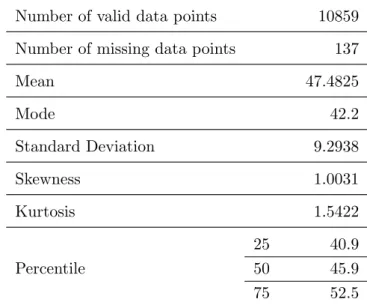
A total of 10,859 women age 15-49 and 3,771 men age 15-54 from 10,400 households cover 361 sample points (clusters) throughout Bangladesh, 134 in urban areas and 227 in the rural areas. The characteristic of weights (dependent variable) and heights (in-dependent variable) of women are given in Table 1 and Table 2, respectively. In order
Table 1: Descriptive statistics of dependent variable (weights) for BDHS 2007 data
Number of valid data points 10859
Number of missing data points 137
Mean 47.4825 Mode 42.2 Standard Deviation 9.2938 Skewness 1.0031 Kurtosis 1.5422 25 40.9 Percentile 50 45.9 75 52.5
Table 2: Descriptive statistics of independent variable (heights) for BDHS 2007 data
Number of valid data points 10859
Number of missing data points 137
Mean 150.5553 Mode 150.5 Standard Deviation 6.5356 Skewness -4.4108 Kurtosis 70.1384 25 146.8 Percentile 50 150.5 75 154.2
to make the relationship (1), we assume that both variables contain measurement error. For examining the accuracy of imputation techniques, we randomly generated 5%, 10%, 20%, 25% and 30% missing data points in dependent variable Y of the complete BDHS 2007 data set (data set without its own 137 missing data points).
3 Results and Discussion
In this section, we compare the different methods of missing values based on simulation study and BDHS2007 data results.
3.1 Comparison of the Different Methods of Missing Values based on Simulation Study
Table 3 demonstrates that for the sample of sizen = 50 at 5% missing values, the EM gives MAE=1.8541 and RMSE= 2.1572 respectively, whereas the mean-before (1.8795 and 2.3844) and the mean-before-after (2.2426 and 2.4920) method give bigger MAE and RMSE values than EM from the simulated data set. Again, when the sample size remains same but the percentage of missing values increase to 10%, 20% and 30%, the EM gives the smallest values of MAE and RMSE than the other two methods. It can be noted that the EM provides almost same values of MAE and RMSE at the different percentage of missing values. However, for the same sample size (n=50), the value of MAE and RMSE increase as the percentage of missing values increase for the methods of mean-before and mean-before-after.
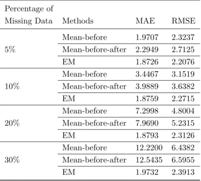
Table 4 also represents the simulation envelope for the various percentage of missing values for the fixed sample size n=70. Like as the simulation results of Table 3, Table 4 shows that the value of MAE and RMSE for EM method are always smaller than the value of the mean-before and mean-before-after method. Again when the percentage of missing values increases, the values of MAE and RMSE for EM differs slightly but the value of MAE and RMSE for the mean-before and the mean-before-after method increases drastically. Moreover, when the sample size varies from 50 to 70 with fixed percentage of missing values (say 10%), the MAE and RMSE of the EM gives almost similar results, whereas it is not true for the mean-before and the mean-before-after methods. A similar conclusion can be made from other percentage of missing values.
Finally, from Table 3 and Table 4, we can say that EM produces the smallest MAE and RMSE than the other two imputation methods for different percentage of missing values and for different sample sizes. It is also observed that the values of MAE and RMSE using the EM method are fairly close with increasing the percentage of missing values. The mean-before and the mean-before-after method, however, show larger values of MAE and RMSE with increasing the percentage of missing values.
Table 3: The MAE and RMSE from three imputation methods forn = 50
Percentage of
Missing Data Methods MAE RMSE
Mean-before 1.8795 2.3844 5% Mean-before-after 2.2426 2.4920 EM 1.8541 2.1572 Mean-before 4.8886 3.6819 10% Mean-before-after 5.6892 4.2681 EM 1.8723 2.2330 Mean-before 10.3717 5.6520 20% Mean-before-after 11.3848 6.1647 EM 1.8894 2.3061 Mean-before 16.1996 7.2737 30% Mean-before-after 17.1567 7.6558 EM 1.8979 2.3414
Table 4: The MAE and RMSE from three imputation methods forn = 70
Percentage of
Missing Data Methods MAE RMSE
Mean-before 1.9707 2.3237 5% Mean-before-after 2.2949 2.7125 EM 1.8726 2.2076 Mean-before 3.4467 3.1519 10% Mean-before-after 3.9889 3.6382 EM 1.8759 2.2715 Mean-before 7.2998 4.8004 20% Mean-before-after 7.9690 5.2315 EM 1.8793 2.3126 Mean-before 12.2200 6.4382 30% Mean-before-after 12.5435 6.5955 EM 1.9732 2.3913
3.2 Comparison of the Different Methods of Missing Values based on BDHS 2007 data
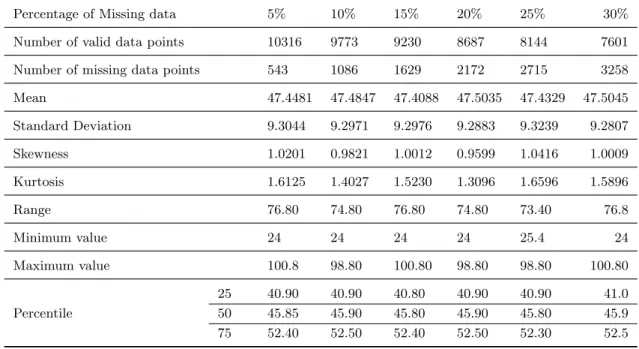
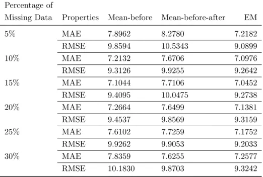
From the simulation study, we get an impression that the EM algorithm outperforms than the other two existing methods for linear structural related variables. The same phenomenon is checked in this section by a practical demographic survey data, BDHS 2007 data. The descriptive statistics for BDHS 2007 data set are shown in Table 5 in which different percentage of missing values are generated. The mean values vary slightly with the percentage of missing data points. In spite of differences in the amount, it is interesting that the analysis generates similar types of results for all percentage of missing values. It can also be seen that there is very small variation in the percentiles with the respective percentage of missing values. This is due to the way in which the missing values were generated, and to the occurrence of a large number of observations within the same range. From Table 6, EM algorithm gives smallest MAE and RMSE for all types of simulated missing data patterns than the other two methods.
Table 5: Descriptive statistics of the dependent variable (weights) for BDHS 2007 data
Percentage of Missing data 5% 10% 15% 20% 25% 30%
Number of valid data points 10316 9773 9230 8687 8144 7601 Number of missing data points 543 1086 1629 2172 2715 3258
Mean 47.4481 47.4847 47.4088 47.5035 47.4329 47.5045 Standard Deviation 9.3044 9.2971 9.2976 9.2883 9.3239 9.2807 Skewness 1.0201 0.9821 1.0012 0.9599 1.0416 1.0009 Kurtosis 1.6125 1.4027 1.5230 1.3096 1.6596 1.5896 Range 76.80 74.80 76.80 74.80 73.40 76.8 Minimum value 24 24 24 24 25.4 24 Maximum value 100.8 98.80 100.80 98.80 98.80 100.80 25 40.90 40.90 40.80 40.90 40.90 41.0 Percentile 50 45.85 45.90 45.80 45.90 45.80 45.9 75 52.40 52.50 52.40 52.50 52.30 52.5
Table 6: The MAE and RMSE from three imputation methods of the dependent variable (weights) for BDHS 2007 data
Percentage of
Missing Data Properties Mean-before Mean-before-after EM
5% MAE 7.8962 8.2780 7.2182 RMSE 9.8594 10.5343 9.0899 10% MAE 7.2132 7.6706 7.0976 RMSE 9.3126 9.9255 9.2642 15% MAE 7.1044 7.7106 7.0452 RMSE 9.4095 10.0475 9.2738 20% MAE 7.2664 7.6499 7.1381 RMSE 9.4537 9.8569 9.3159 25% MAE 7.6102 7.7259 7.1752 RMSE 9.9262 9.9053 9.2033 30% MAE 7.8359 7.6255 7.2577 RMSE 10.1830 9.8703 9.3242
4 Conclusions
In this article, different imputation methods are compared to handle the missing data in linear structural relationship model. Two performance indicators namely MAE and RMSE are used to find the most effective imputation method. Based on the simulated data set, it is observed that the EM method performs better than the other two impu-tation methods to impute missing data in LSRM as it produces the smallest MAE and RMSE. It is also observed that EM method produces relatively same values for MAE and RMSE, whereas the mean-before and mean-before-after method show an increasing pattern in MAE and RMSE when the percentage of missing values are increased. Similar conclusions can be made for real BDHS2007 data set that the EM performs better than the other two imputation methods.
Acknowledgement
The authors are thankful to the Referees and Editor for their very helpful comments and suggestions.
References
Ayyub, B. M. and McCuen, R. H. (1996). Probability, statistics and reliability for engineers and scientists. Springer.
Carpita, M. and Ciavolino, E. (2016). A generalized maximum entropy estimator to simple linear measurement error model with a composite indicator. Advances in data analysis and classification.Available on: DOI: 10.1007/s11634-016-0237-y.
Carpita, M. and Ciavolino, E. (2015). The GME estimator for the regression model with a composite indicator as explanatory variable. Quality and Quantity, 49(3), 955–965. Chen, J. L., Islam, S., and Biswas, P. (1998). Nonlinear dynamics of hourly ozone concentrations:Nonparametric short term prediction. Atmospheric Environment, 32, 39–48.
Dempster, A. P., Laird, N. M., and Rubin, D. B. (1977). Maximum likelihood from incomplete data via EM algorithm. Journal of the Royal Statistical Society. Series B (Methodological), 39(1), 1–38.
Gaetan, C. and Yao, J. F. (2003). A multiple imputation metropolis version of the EM algorithm. Biometrika, 90(3), 643–654.
Geng, Z., Wan, K. and Tao, F. (2000). Mixed graphical models with missing data and the partial imputation EM algorithm. Scandinavian Journal of Statistics, 27(3), 433–444. Hippel, P. T. V. (2004). Biases in SPSS 12.0 missing value analysis. The American
Statistician, 58(2), 160–164.
Hood K., Barry A. J. Nix, and Terence C. Iles (1999). Asymptotic information and variance-covariance matrices for the linear structural model. The Statistician, 48, 477–493.
Junninen, H., Niska, H., Tuppurrainen, K., and Ruuskanen, J. (2004). Methods for imputation of missing values in air quality data sets. Atmospheric Environment,38, 895–907.
Kendall, M.G. and Stuart, A. (1973).The Advance Theory of Statistics. London, Griffin.
Kofmanhttp, P., and Sharpe, I. (2000). Imputation
Meth-ods for Incomplete Dependent Variables in Finance. Available on://www.econometricsociety.org/meetings/wc00/pdf/0409.pdf.
Little, R. J. A, and Rubin, B. B. (1987). Statistical analysis with missing data. New York: Wiley.
Little, R. J. A, and Rubin, B. B. (2002). Statistical analysis with missing data. New York: Wiley.
NIPORT. (2009). Bangladesh Demographic and Health Survey 2007. Dhaka, Bangladesh and Calverton, Maryland, USA: National Institute of Population Research and Train-ing, Mitra and Associates, and Macro International. National Institute of Population Research and Training, Mitra and Associates, and Macro International.
Norazian, M. N., Shukri, Y. A., Azam, R.N. and Al Bakri, A.M.M. (2008). Estimation of missing values in air pollution data using single imputation techniques.ScienceAsia,34,
341–345.
Perneger, T. V., and Burnand, B. (2005). A simple imputation algorithm reduced missing data in SF-12 health surveys. Journal of Clinical Epidemiology, 90(3), 643–654. Sundberg, R. (1974). Maximum likelihood theory for incomplete data from an
exponen-tial family. Scandinavian Journal of Statistics, 1(2), 49–58.
Twisk, J., and Vente, W. (2001). Attrition in longitudinal studies: How to deal with missing data. Journal of Clinical Epidemiology, 55, 329–337.
Winkler, A. and McCarthy, P. (2005). Maximising the value of missing data. Journal of Targeting, Measurement and Analysis for Marketing, 13(2), 168–178.
Wu, C. F. J. (1983). On the convergence properties of the EM algorithm. The Annals of Statistics, 11(1), 95–103.
Yahaya, A.S., Ramli, N.A., and Yusof, N.F. (2005). Effects of estimating missing values on fitting distributions. Proceedings of the International conference on quantitative sciences and its applications, Penang, Malaysia.