(www.interscience.wiley.com) DOI: 10.1002/sim.0000
Using a monotone single-index model to stabilize
the propensity score in missing data problems
and causal inference
Jing Qin
1, Tao Yu
2, Pengfei Li
3, Hao Liu
4and Baojiang Chen
5∗The augmented inverse weighting method is one of the most popular methods for estimating the mean of the response in causal inference and missing data problems. An important component of this method is the propensity score. Popular parametric models for the propensity score include the logistic, probit, and complementary log-log models. A common feature of these models is that the propensity score is a monotonic function of a linear combination of the explanatory variables. To avoid the need to choose a model, we model the propensity score via a semiparametric single-index model, in which the score is an unknown monotonic nondecreasing function of the given single index. Under this new model, the augmented inverse weighting estimator of the mean of the response is asymptotically linear, semiparametrically efficient, and more robust than existing estimators. Moreover, we have made a surprising observation. The inverse probability weighting and augmented inverse weighting estimators based on a correctly specified parametric model may have worse performance than their counterparts based on a nonparametric model. A heuristic explanation of this phenomenon is provided. A real-data example is used to illustrate the proposed methods. Copyright c⃝2017 John Wiley & Sons, Ltd.
Keywords: Causal inference; Empirical process; Inverse weighting; Missing data; Pool adjacent violation algorithm; Single-index model.
1. Introduction
Causal inference and missing data problems have been extensively researched in recent decades in medical, social and economical sciences (e.g., [1,2,3, 4, 5,6,7, 8, 9]). Consider a medical experiment with n subjects where each subject is assigned to either the treatment or the control group. Denote byYi (Ti) the outcome variable for subject i,
if it was assigned to the treatment (control) group. At the end of the study, we observeYi orTi but not both. LetXi
and ∆i be the corresponding baseline covariates and the treatment indicator respectively;∆i= 1 if the ith patient is
assigned to the treatment group and thereforeYi is observed, and∆i= 0otherwise. In summary, the data are denoted
(Yi, Ti,∆i, Xi), i= 1, . . . , n.
We wish to estimateµ=E(Yi)andν=E(Ti). In the aforementioned medical study, the meanings of these quantities
are clear. For example,µis the population average of the response for the patients in the treatment group. This estimation problem has applications in social science, medical research, economic studies, and other fields (e.g., [1], [2]). For presentational convenience, we will focus on estimation methods forµ; those forνcan be similarly established. Therefore, the observed data are(∆iYi,∆i, Xi),i= 1, . . . , n.
We now briefly review existing methods for the estimation ofµ. An important quantity is the propensity score, defined to beπ(x) =P(∆ = 1|X =x), which is the probability that a subject will be assigned to the treatment group, given the
1National Institute of Allergy and Infectious Diseases, National Institute of Health, Bethesda, MD 20892, US 2Department of Statistics & Applied Probability, National University of Singapore, 117546, Singapore 3Department of Statistics and Actuarial Sciences, University of Waterloo, Waterloo, ON, N2L 3G1, Canada 4Department of Biostatistics, Indiana University School of Medicine, Indianapolis, IN 46202, USA
5Department of Biostatistics and Data Science, University of Texas Health Science Center at Houston, School of Public Health in Austin, Austin, 78701 U.S.A.
∗Correspondence to: Baojiang Chen, email: [email protected]
____________________________________________________
observed covariateX=x. The importance ofπ(x)in the estimation ofµhas been discussed by Rosenbaum and Rubin [11]. In this article, we assume0< π(x)<1to avoid potential technical difficulties.
One popular estimator ofµis the inverse probability weighting estimator ([12]), defined to be b µHT(π(·)) = 1 n n ∑ i=1 ∆iYi π(Xi) . (1)
However, this estimator has a counterintuitive feature ([13]): ifπ(x)takes the parametric formπ(x;β), withπ(x;β)being a known function up to an unknown parameterβ, thenbµHT(π(·;βb))could be a more efficient estimator thanµbHT(π(·;β0)).
Hereβbandβ0denote the maximum likelihood estimator and the true value ofβ, respectively.
Theaugmented inverse weighting estimator(AIWE; [14]) improves the performance ofµbHT by augmenting aworking
modelψ(·)of the response on the covariates; it does not have the above counterintuitive feature. The AIWE is given by b µ(π(·), ψ(·)) = 1 n n ∑ i=1 { ∆iYi π(Xi)− ∆i−π(Xi) π(Xi) ψ(Xi) } . (2)
A common choice of the working model isψ(x) =E(Y|X =x). Clearly, the performance ofµb(π(·), ψ(·))relies heavily on the choice ofπ(·)andψ(·). Scharfstein, Rotnitzky, and Robins [15] noted that this estimator is doubly robust in that it is consistent if one of the models for estimatingπandψ, but not both, is misspecified. Wooldridge [16] and Uysalc[17] applied this method in treatment effects models. Sloczynski and Wooldridge [18] provided a unified framework for various doubly robust estimators of the average treatment effect under unconfoundedness. However, Kang and Schafer [19] demonstrated via numerical studies that this estimator can be severely biased if both models are misspecified. Therefore, it is important to specify a flexible but correct model for at least one ofπandψ. Given the importance of the propensity score, we propose a novel and flexible semiparametric model forπ(x)and study the asymptotic properties of the AIWE ofµ.
Note thatπ(·)can be viewed as a regression model for the binary response data(∆i, Xi), i= 1, . . . , n, where the∆i’s
are the response and theXi’s are the covariates. A popular model forπ(·)is the well-known logistic model:
log π(x) 1−π(x) =x
Tβ.
The probit and complementary log-log models are also widely used for binary response data. The common feature of these parametric models is thatπ(x)is latently assumed to be a monotonic function of a linear combination of the explanatory variables, i.e.,xTβ. To avoid the need to choose a model, we modelπ(x)as a monotonic function ofhT(x)β, withh(x)
being a user-specified function. In particular, we propose the following semiparametric single-index model:
π(x) =θ(hT(x)β), (3) where bothθ(·)andβare unknown, andθ(·)is a monotonic nondecreasing function. Since the form ofθ(·)is not specified, our model is more flexible than parametric models.
Under the setup (3), we consider the estimation ofµwithin the framework of the AIWE. We first propose to estimate
θ(·)andβby the maximum likelihood method. Compared with the nonparametric methods for estimatingπ(x)(e.g., [20], [5]), our methods do not need tuning parameters. In our numerical studies, we observe that our methods are more accurate in estimating the AIWEs than the nonparametric methods if the linear predictors in the propensity score is correctly specified. Another limitation of the nonparametric methods is the curse of dimensionality: the estimates forπ(x)may not perform well when the dimension ofxis relatively large; in contrast, our proposed methods do not suffer this problem. Compared with the parametric methods (e.g., the logistic regression method) for estimatingπ(x), our methods are more robust. We then consider the estimation ofψin broad function classes via the weighted least square principle. We show theoretically that with our proposedπestimator and the generalψestimator based on broad function classes, the AIWE is asymptotically linear and can achieve semiparametric efficiency. We observe that because of the non-smoothness of our estimators forπ(x), the existing asymptotic theory in the community is not directly applicable to our estimators; the theoretical developments for the linear expansion and the efficiency are nontrivial. Furthermore, we present extensive numerical studies to demonstrate that our estimator has better accuracy than existing estimators.
The organization of the paper is as follows. In Section 2, we present the methods for estimatingπ(·)under the setup (3) withψbased on broad function classes. In Section 3, we investigate the asymptotic properties of the AIWE based on the proposed semiparametric model. Sections 4 and 5 present the simulation results and a real application, respectively. Section 6 provides concluding remarks. For convenience of presentation, the technical details are given in the Appendix.
2. Estimation Methods for
π
(
·
)
and
ψ
(
·
)
In this section, we discuss estimation methods forπ(·)andψ(·). We first consider the estimation ofπ(·)by the maximum likelihood method. We then discuss the estimation ofψin broad function classes with the weighted least square principle.
2.1. Estimation Methods forπ
Recall that the estimation ofπ(·)can be established by appropriately modeling the binary response data (∆i, Xi), i=
1, . . . , n. Specifically, we consider the maximum likelihood method. The log-likelihood based on(∆i, Xi), i= 1, . . . , nis
given by ℓ(π(·)) = n ∑ i=1 [ ∆ilog{π(Xi)}+ (1−∆i) log{1−π(Xi)} ] , (4)
and the maximum likelihood estimator ofπ(·)is defined to be b
π=argmaxπ∈Fℓ(π(·)), (5)
whereFis a prespecified function class forπ. Clearly,F plays a central role in determining the asymptotic performance ofbπ(·).
Under the semiparametric single-index model (3) forπ(·), the log-likelihood function becomes
ℓ(θ, β) = n ∑ i=1 [ ∆ilog{θ(hT(Xi)β)}+ (1−∆i) log{1−θ(hT(Xi)β)} ] . (6)
Without loss of generality, we assume hereafter thatθ(·)is monotonically increasing. Furthermore, we assumeβ1= 1so
that the model is identifiable, although in principle other assumptions can be made for identifiability. Then the maximum likelihood estimators forθ(·)andβare defined as
(θ,bβb) =argmaxθ∈Θ,β∈Λℓ(θ, β), (7) where Θ ={θ(·) : 0≤θ(x)≤1is monotone inx∈R} and Λ ={1} ×Λ−1 are the parameter spaces for θ(·) and β,
respectively.
A numerical algorithm for the optimization problem (7) can be established using a similar strategy to that of Cosslett [21]; see also Chen et al. [22] and the references therein. Specifically, we implement the following two-stage algorithm to computeθb(·)andβb.
Stage 1. For a givenβ, profileθ(·)to obtain the profile likelihood ofβthrough the following steps:
(a) Let(v1(β), . . . , vn(β))be a vector composed of{hT(Xi)β:i= 1, . . . , n}, and sort the entries from smallest
to largest:
v(1)(β)≤. . .≤v(n)(β).
The corresponding∆i’s are denoted∆1(β), . . . ,∆n(β). Substitutev(i)(β)and the corresponding∆i(β)into
(6) to obtain ℓ(θ, β) = n ∑ i=1 [ ∆i(β) log{θ(v(i)(β))}+{1−∆i(β)}log{1−θ(v(i)(β))} ] .
(b) For anyβand theℓ(θ, β)given in (a), let b
θβ=argmaxθ∈Θℓ(θ, β). (8)
Following Dykstra, Kochar, and Robertson [23], solve the maximum problem using the well-known pool-adjacent-violation-algorithm (PAVA; [24]).
(c) Find the profile log-likelihood via
ℓ(θbβ, β) = n ∑ i=1 [ ∆ilog{θbβ(hT(Xi)β)}+ (1−∆i) log{1−bθβ(hT(Xi)β)} ] . (9)
Stage 2. Maximize (9) with respect toβ to obtainβb. This step can be implemented using software such as the R function optim() ([25]) with the given initial value ofβ. Thenbθ(·) =bθβb(·).
Consequently, we can estimateπ(x)bybπ(x) =bθ(hT(x)βb). The following theorem establishes the convergence rate of b
π(x)to its true valueπ0(x) =θ0(hT(x)β0), whereθ0(·)is monotonically increasing and is the true value ofθ(·), andβ
0
is the true value ofβ.
Theorem 1 LetPbe a probability measure. Assuming Conditions 1–3 in the Appendix, we have
∥bπ−π0∥2,P=Op(n−1/3),
where∥ · ∥2,Pdenotes theL2norm under the probability measureP, specifically, for any measurable functionf, ∥f∥2,P=
(∫
f2dP
)1/2
.
The proposed algorithm performs well when the dimension of β is small or moderate. However, it becomes computationally expensive when this dimension is relatively large. The reason is twofold. First, it involves a two-stage iteration. Second, the profile likelihood given in (8) is not smooth in the neighborhood ofβb. On the other hand, in our theoretical development and numerical studies, we observe that the estimate ofµis robust to the estimate ofβif it is not too far fromβb. Intuitively, this is becausebµ(π(·), ψ(·))is a smooth function ofbπ(·). In practice, when the dimension ofβ
is relatively large, one could implement the following much faster algorithm instead of the two-stage algorithm above. Step 1. Given the binary response data(∆i, Xi), i= 1, . . . , n, obtain βbby fitting a parametric model, say a logistic
regression model.
Step 2. Similarly to Stage 1(b), estimateθusing the classical PAVA algorithm and the data(∆i, hT(Xi)βb),i= 1, . . . , n.
The extensive numerical studies in Section4show that the inverse probability weighting estimatorbµHT(π(·))withbπ(·)
from our method leads to more robustµ estimates than that based onπb(·) from the parametric methods, even though the assumed parametric model is correct. We now give an intuitive explanation of this observation. Consider the case where∆i= 1but the correspondingπ0(Xi)is very close to 0. This may occur occasionally ([26]); in our simulation, with
n= 1000observations and 1000 replications, this is likely to occur at least once. In this scenario the parametric estimate ofπ(·), denotedπ(·;βb), is likely also close to 0, because it is a consistent estimator ofπ0(·). In our simulation,π0(·)and
π(·;βb)can be as small as9×10−7. Sinceπ(·)appears in the denominator in the estimatorµbHT(π(·))—see (1)—these
observations may significantly affect the accuracy ofµbHT(π(·;βb)). With our proposedπb(·)estimate, however,µbHT(bπ(·))
is much more robust. This is because when∆i= 1, the correspondingθb(hT(Xi)βb)from the PAVA algorithm is greater
than1/n. Therefore, the accuracy ofµbHT(bπ(·))is much less affected by any individual observation.
2.2. Estimation Methods forψ
Estimation methods forψ(·)have been widely discussed (e.g., [27], [14], [15]). In this paper, we generally consider the weighted least square objective function given by
Q(ψ) =
n ∑
i=1
w(∆i, Xi){Yi−ψ(Xi)}2,
wherew(∆i, Xi)is the user-specified weight function. Assume thatψis estimated by b
ψ=argminψ∈ΨQ(ψ), (10)
whereΨdenotes the class of functions for the “guessed” working model.
Cao, Tsiatis, and Davidian [27] suggest the following parametric model forψ(·)and form forw(·,·):
(1) ψ(x) =h(x;γ), withha known function andγ the unknown Euclidean parameter. Therefore,Ψ ={ψ:ψ(x) =
h(x;γ), γ∈Rk}, wherekis the dimension ofγ.
(2) w(δ, x) = δ{1πb−2bπ(x()x)}, wherebπis obtained from (5).
3. Asymptotic Behavior of the Augmented Inverse Weighting Estimator
With the estimatorsπbandψbgiven in the last section, the AIWE ofµis given by b µ(bπ(·),ψb(·)) = 1 n { n ∑ i=1 ∆iYi b π(Xi)− ∆i−bπ(Xi) b π(Xi) b ψ(Xi) } = Pnϕ(v;µ0,bπ(·),ψb(·)) +µ0, (11) wherev= (δ, y, xT)T, ϕ(v;µ, π(·), ψ(·)) = δy π(x)− δ−π(x) π(x) ψ(x)−µ,
and Pn is an empirical measure such that Png(v) = ∫
g(v)dPn for any function g(v). For simplicity, we denote this
estimator asµbwhen the context is clear.
We first explore the asymptotic behavior ofµbwhenbπandψbare assumed to be estimated from (5) and (10) respectively. The asymptotic behavior ofπband ψbare significantly affected by the complexity of the function classesF andΨ. The following entropy conditions, which combine the main parts of Conditions A and B in the Appendix, play key roles in the proof of Theorem2.
Entropy Conditions: There exist0< α1, α2<2such that for everyϵ >0
H2,B(ϵ,F, FX)< A1ϵ−α1 and H2,B(ϵ,Ψ, FX)< A2ϵ−α2,
whereFXdenotes the cumulative distribution function of the covariatesX, andA1andA2are universal constants.
HereH2,B(ϵ,F, FX)is theϵ-entropy with bracketing ofF, which is commonly adopted in empirical process texts. We
give a quick review ofH2,B(ϵ,F, FX)in the Appendix.
Theorem 2 Letψ0(x)be the true value ofψ(x). Assuming Conditions A–C in the Appendix, we have
√ n(µb−µ0)−√nPnϕ(v;µ0, π0, ψ0) + √ nP [{ π0(x) b π(x) −1 } { b ψ(x)−ψ0(x) }] = Op ( ∥πb−π0∥ 1−α1/2 2,P ) +Op ( ∥ψb−ψ0∥ 1−max{α1,α2}/2 2,P ) +op(1), (12)
wherePg(v) =∫ g(v)dPfor any functiong(v).
Corollary 1 Assuming Conditions A–C in the Appendix, we have (P1) if √ nP [{ π0(x) b π(x) −1 } { b ψ(x)−ψ0(x) }] =Op(1), thenµb−µ0=Op(n−1/2); (P2) if∥bπ−π0∥2,P=op(1),∥ψb−ψ0∥2,P=op(1), and √ nP [{ π0(x) b π(x) −1 } { b ψ(x)−ψ0(x) }] =op(1), then√n(µb−µ0) = √
nPnϕ(v;µ0, π0, ψ0) +op(1), andµbachieves the semiparametric information bound.
Remark 1 In the development of Theorem2and Corollary1, we do not require thatπ0∈ Fandψ0∈Ψ. That is, Models
(5) and (10) need not be the true models ofπandψ.
Remark 2 Calculations for entropies of function classes are available in empirical process texts. Based on these, the entropy conditionH2,B≤Aϵ−α for some universal constant A and0< α <2 accommodates many “good” function
classes. For example, for most parametric models, the corresponding function classes satisfy this condition withα >0; the class of bounded monotone functions satisfies this condition with α= 1; the function class with every element g
satisfyingg: [0,1]→[0,1]such that∫01{g(m)(x)}2dx≤1satisfies this condition withα= 1/m. See Section 2.2 of van
de Geer [28], Sections 2.6 and 2.7 of van der Vaart and Wellner [29], Chapter 9 of Kosorok [30], and the references therein for more classes of functions that satisfy this entropy condition.
Theorem 3 Letbπ(x) =θb(hT(x)βb), where(bθ,βb)are obtained from (7). Assume Conditions 1–3, and B–E in the Appendix.
We have
√
n(µb−µ0)−√nPnϕ(v;µ0, π0, ψ0) =op(1).
Remark 3 From this theorem, we observe that in our method the estimatorµbis semiparametrically efficient under mild regularity conditions. The main regularity conditions are (1)π0(x)is monotone, and (2)ψ0(x)belongs to a function class that satisfies a mild entropy condition, say ConditionB1. Furthermore, if the parametric model and the single-index model (3) forπ(x)are both correctly specified, our method and the AIWE based on the correctly specified parametric model have the same efficiency. This is true even when we obtain the estimate ofπ(x)via the second algorithm in Section 2.1, where we first obtain the estimate βbby fitting a parametric model and then estimate θ(·)using the PAVA based on the data
(∆i, h(Xi)Tβb), i= 1, . . . , n. That is, compared with the AIWE based on the correctly specified parametric model, our
method does not lose any efficiency provided the single-index model is correctly specified. If this condition is not satisfied, our estimator is root-nconsistent given the even more mild condition required by (P1) of Corollary1. In particular, ourµb
maintains the double robustness property as desired and is more robust than the AIWE based on the parametric model.
4. Simulation Studies
In this section we conduct simulation studies to explore the performance of the proposed estimators. We consider the following eight estimators:
1) The inverse probability weighting estimator (1) withπ(x)estimated by the logistic regression model reviewed in Section2.1; we call this methodHT-par.
2) The inverse probability weighting estimator withπ(·)estimated by the semiparametric method proposed in Section 2.1, i.e.,π(x) =θ(hT(x)β). Here we use the second algorithm in Section2.1to estimateπ(·). We call this method
HT-pava.
3) The H´ajek inverse probability weighting estimator ([31]), withπ(x)estimated as inHT-pava; we call this method
HAJ-pava. In particular, b µHAJ-pava= ∑n i=1∆iYi/πb(Xi) ∑n i=1∆i/bπ(Xi) .
4) The estimatorbµPROJproposed in Cao, Tsiatis, and Davidian [27]; we call this methodCao-proj.
5) The AIWE withπ(x)estimated by the using the generalized additive model [10] andψ(x)estimated by the method presented in Section2.2; we call this methodNP-AIWE. Specifically, we consider the following nonparametric model for estimating the propensity score:
logit{P(∆ = 1|x1, . . . , xp)}= p ∑ j=1
hj(xj),
wherehj(·),j= 1, . . . , pare nonparametric functions; the natural cubic-spline is applied to estimate them.
6) The propensity score matching method ([11]) using different number of cutpointsJ; we call this methodPSM-J. In this study, we useJ = 5,10, and20.
7) The AIWE withπ(x)estimated by the first algorithm in Section2.1andψ(x)estimated by the method presented in Section2.2; we call this methodNew-pava1.
8) The AIWE withπ(x)estimated by the second algorithm in Section2.1andψ(x)estimated by the method presented in Section2.2; we call this methodNew-pava2.
We consider three examples.
Example 1. We first consider the artificial example created by Kang and Schafer [19]. In this scenario, for each
i(i= 1, ..., n), Zi= (Zi1, Zi2, Zi3, Zi4)Tis generated as standard multivariate normal random variables, and the elements
of Xi= (Xi1, Xi2, Xi3, Xi4)T are defined asXi1= exp(Zi1/2), Xi2=Zi2/{1 + exp(Zi1)}+ 10, Xi3= (Zi1Zi3/25 + 0.6)3, andX
i4= (Zi2+Zi4+ 20)2, so thatZimay be expressed in terms ofXi. For eachi,
Yi = 210 + 27.4Zi1+ 13.7Zi2+ 13.7Zi3+ 13.7Zi4+ϵi,
whereϵi is independent standard normal, and ∆i is generated as a Bernoulli random variable with the true propensity
score being
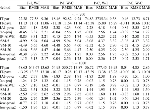
Table 1. Comparison of the bias, RMSE, and MAE for the estimates ofµin Example 1. Here “P-C” (or “P-I”) indicates that the model forπ(·)is correctly (or incorrectly) specified; “W-C” (or “W-I”) indicates that the model forψ(·)is correctly
(or incorrectly) specified.
P-I, W-I P-I, W-C P-C, W-I P-C, W-C
Method Bias RMSE MAE Bias RMSE MAE Bias RMSE MAE Bias RMSE MAE
n= 200 HT-par 22.28 77.58 9.36 18.46 92.82 9.24 74.83 3735.34 9.38 -0.46 12.73 6.71 HT-pava 11.13 11.61 11.06 -11.18 11.64 11.14 -15.38 15.80 15.29 -10.11 10.66 10.16 HAJ-pava -2.31 4.18 2.95 -2.38 4.23 3.00 -2.28 4.18 3.01 -0.84 3.55 2.37 Cao-proj -0.45 3.37 2.21 -0.04 2.56 1.75 -0.00 2.56 1.74 -0.02 2.54 1.72 NP-AIWE -0.83 3.31 2.21 -0.15 2.55 1.74 -0.55 3.23 2.22 -0.16 2.58 1.77 PSM-5 -4.99 5.94 5.04 -4.99 5.94 5.04 -3.08 4.37 3.32 -3.08 4.37 3.32 PSM-10 -4.49 5.65 4.60 -4.48 5.65 4.60 -2.52 4.15 2.90 -2.52 4.15 2.90 PSM-20 -4.46 5.66 4.47 -4.46 5.66 4.47 -2.50 4.25 2.99 -2.50 4.25 2.99 New-pava1 -0.38 3.29 2.22 -0.04 2.56 1.75 0.00 2.56 1.73 -0.02 2.53 1.71 New-pava2 -1.15 3.13 2.17 -0.04 2.56 1.75 0.00 2.56 1.75 -0.02 2.53 1.71 n= 1000 HT-par 48.63 643.67 13.63 54.93 530.75 13.87 36.72 177.45 13.93 0.04 4.85 2.86 HT-pava -13.25 13.33 13.30 -10.17 10.28 10.17 -13.29 13.38 13.28 -10.00 10.13 10.01 HAJ-pava -1.82 2.37 1.86 -1.83 2.38 1.91 -1.83 2.38 1.88 -0.20 1.51 1.00 Cao-proj -1.24 1.78 1.32 -0.01 1.15 0.78 -0.02 1.15 0.78 0.00 1.13 0.78 NP-AIWE -1.57 2.10 1.62 -0.01 1.14 0.77 -0.19 1.46 0.98 -0.02 1.13 0.76 PSM-5 -3.22 3.51 3.24 -3.22 3.51 3.24 -1.44 1.95 1.50 -1.44 1.95 1.50 PSM-10 -2.59 2.96 2.62 -2.59 2.96 2.62 -0.83 1.60 1.11 -0.83 1.60 1.11 PSM-20 -2.36 2.76 2.39 -2.36 2.76 2.39 -0.60 1.54 1.02 -0.60 1.54 1.02 New-pava1 -0.77 1.72 1.18 -0.01 1.15 0.77 -0.02 1.15 0.78 0.00 1.13 0.78 New-pava2 -1.50 1.96 1.51 -0.01 1.15 0.77 -0.02 1.15 0.78 0.00 1.13 0.78
where logit(t) = log{t/(1−t)}fort∈(0,1). The true value ofµisµ0= 210.
If we fit a linear regression model forYi overZiand a logistic regression model for∆ioverZi, then the models for
ψ(·)andπ(·)are correctly specified. However, ifZiis replaced byXiin the above fitted models, then the models forψ(·)
andπ(·)are incorrectly specified. In total, we have four combinations of model specifications forψ(·)andπ(·). For each combination, we calculate the bias, square root mean square error (RMSE), and median absolute error (MAE) of the ten estimates ofµbased on 5000 repetitions. We consider two sample sizes, 200 and 1000; the results are reported in Table1. We make the following observations:
• Clearly, Cao-proj, New-pava1, and New-pava2 have similar performance. They perform better than the other estimators.
• NP-AIWE performs comparable or slightly worse than our methods.
• HT-pavahas a much smaller RMSE than its counterpartHT-par. However, the MAEs are comparable forn= 200.
• AlthoughHAJ-pavadoes not use the working regression model, its performance is close to that ofCao-projand the new estimators.
To illustrate the robustness of our methods, we give two further examples.
Example 2. The “working” propensity score function is given by the logistic regression logit{P(∆ = 1|x1, x2)}=
β0+β1x1+β2x2. The true propensity score is given by the following three models:
Model I:
logit{P(∆ = 1|x1, x2)}= 2x1−x2.
In this case the propensity score is correctly specified. Model II:
logit{P(∆ = 1|x1, x2)}= 2x1−x2+ 2x21;
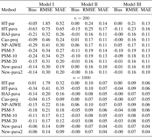
Table 2. Comparison of the bias, RMSE, and MAE for the estimates ofµin Example 2.
Model I Model II Model III
Method Bias RMSE MAE Bias RMSE MAE Bias RMSE MAE
n= 200 HT-par -0.05 1.85 0.52 0.00 0.24 0.14 0.00 0.21 0.13 HT-pava -0.63 0.75 0.65 -0.15 0.25 0.17 -0.11 0.23 0.16 HAJ-pava -0.21 0.32 0.26 -0.01 0.16 0.11 -0.00 0.16 0.11 Cao-proj -0.09 0.46 0.24 0.01 0.17 0.11 -0.00 0.16 0.11 NP-AIWE -0.29 0.41 0.30 0.06 0.17 0.11 0.05 0.17 0.11 PSM-5 -0.24 0.34 0.27 -0.11 0.19 0.14 -0.10 0.19 0.13 PSM-10 -0.24 0.34 0.25 -0.10 0.19 0.13 -0.09 0.18 0.13 PSM-20 -0.15 0.31 0.20 -0.01 0.16 0.11 -0.01 0.16 0.11 New-pava1 -0.14 0.30 0.19 0.00 0.16 0.10 -0.01 0.16 0.10 New-pava2 -0.14 0.30 0.20 -0.00 0.16 0.11 -0.01 0.16 0.10 n= 1000 HT-par 0.01 1.79 0.32 0.00 0.10 0.07 0.00 0.09 0.06 HT-pava -0.34 0.41 0.35 -0.05 0.10 0.07 -0.04 0.09 0.06 HAJ-pava -0.14 0.20 0.16 -0.00 0.08 0.05 -0.00 0.07 0.05 Cao-proj -0.04 0.15 0.09 0.00 0.07 0.05 -0.00 0.07 0.05 NP-AIWE -0.15 0.22 0.16 0.06 0.10 0.07 0.05 0.09 0.06 PSM-5 -0.18 0.21 0.18 -0.05 0.09 0.06 -0.04 0.08 0.06 PSM-10 -0.11 0.17 0.12 -0.03 0.08 0.05 -0.03 0.08 0.05 PSM-20 -0.11 0.17 0.12 -0.03 0.08 0.05 -0.03 0.08 0.05 New-pava1 -0.06 0.14 0.09 -0.00 0.07 0.04 -0.01 0.07 0.04 New-pava2 -0.06 0.14 0.09 -0.00 0.07 0.04 -0.00 0.07 0.04 Model III: logit{P(∆ = 1|x1, x2)}= 2x1−x2−x1x2+ 2x21.
An interaction term and a quadratic term are missing. The regression model forY is given by
Y = 3 +x21+x2+ϵ,
wherex1,x2, andϵare independent standard normal random variables. Hence, the true value ofµisµ0= 4. The “working
model” is
ψ(x) =γ0+γ1x1+γ2x2.
For the proposed methods, the parameters are estimated by the weighted least square method described in Section 2.2. We again consider two sample sizes:n= 200,1000. Table2gives the bias, RMSE, and MAE of all the estimates ofµ
for5000repetitions in Table2. We make the following observations:
• For model I, where the propensity score is correctly specified, the proposed New-pava1, New-pava2 methods perform better than the other methods.
• For models II and III, where the propensity score is misspecified, the proposed methods perform comparable or slightly better than other methods.
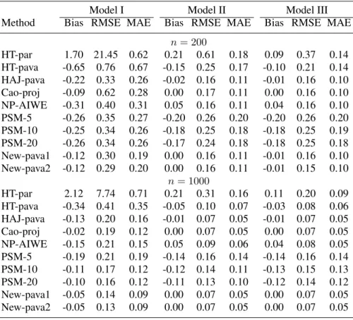
Example 3. To evaluate the robustness of the proposed method to the misspecification of the link function in the propensity score, we consider the following example. The setup is the same as in example 2, except that we posit the following propensity models
Model I:
log[−log{1−P(∆ = 1|x1, x2)}] = 2x1−x2;
Model II:
Table 3. Comparison of the bias, RMSE, and MAE for the estimates ofµin Example 3.
Model I Model II Model III
Method Bias RMSE MAE Bias RMSE MAE Bias RMSE MAE
n= 200 HT-par 1.70 21.45 0.62 0.21 0.61 0.18 0.09 0.37 0.14 HT-pava -0.65 0.76 0.67 -0.15 0.25 0.17 -0.10 0.21 0.14 HAJ-pava -0.22 0.33 0.26 -0.02 0.16 0.11 -0.01 0.16 0.10 Cao-proj -0.09 0.62 0.28 0.00 0.17 0.11 0.00 0.16 0.10 NP-AIWE -0.31 0.40 0.31 0.05 0.16 0.11 0.04 0.16 0.10 PSM-5 -0.26 0.35 0.27 -0.20 0.26 0.20 -0.20 0.26 0.20 PSM-10 -0.25 0.34 0.26 -0.18 0.25 0.18 -0.18 0.25 0.19 PSM-20 -0.26 0.34 0.26 -0.17 0.24 0.18 -0.18 0.25 0.18 New-pava1 -0.12 0.30 0.19 0.00 0.16 0.11 -0.01 0.16 0.10 New-pava2 -0.12 0.29 0.20 0.00 0.16 0.11 -0.01 0.15 0.10 n= 1000 HT-par 2.12 7.74 0.71 0.21 0.31 0.16 0.11 0.20 0.09 HT-pava -0.34 0.41 0.35 -0.05 0.10 0.07 -0.03 0.08 0.06 HAJ-pava -0.13 0.20 0.16 -0.01 0.07 0.05 -0.01 0.07 0.05 Cao-proj -0.02 0.19 0.12 0.00 0.07 0.05 0.00 0.07 0.05 NP-AIWE -0.15 0.21 0.15 0.05 0.09 0.06 0.04 0.08 0.05 PSM-5 -0.19 0.21 0.19 -0.14 0.16 0.14 -0.14 0.16 0.14 PSM-10 -0.11 0.17 0.12 -0.12 0.14 0.11 -0.13 0.15 0.13 PSM-20 -0.10 0.16 0.12 -0.11 0.13 0.10 -0.12 0.14 0.12 New-pava1 -0.05 0.14 0.09 0.00 0.07 0.05 0.00 0.07 0.05 New-pava2 -0.05 0.13 0.09 0.00 0.07 0.05 0.00 0.07 0.05 Model III: log[−log{1−P(∆ = 1|x1, x2)}] = 2x1−x2−x1x2+ 2x21.
Table3gives the results for 5000repetitions. Similar scenarios to Example 2 are observed; the details are omitted for brevity.
5. Applications
In this section, we apply our methods to the AIDS Clinical Trials Group Study 175 (ACTG 175; [32]). ACTG 175 is a randomized clinical trial comparing monotherapy (zidovudine or didanosine) with combination therapy (zidovudine and didanosine, or zidovudine and zalcitabine) in adults infected with the type-I HIV virus with CD4 T cell counts between 200 and 500 per cubic millimeter. The study included 2139 HIV-positive subjects. These subjects were followed for about 96 weeks, and the CD4 T cell counts were measured at week 20 and week 96. Some cell counts at week 96 were missing because of subject dropout; the missing proportion is 37.3%. The baseline covariates and the week-20 counts were always observed. The covariates include: age at baseline (in years), weight at baseline (in kg), hemophilia (0=no, 1=yes), homosexual activity (0=no, 1=yes), history of intravenous drug use (0=no, 1=yes), Karnofsky score (on a scale of 0–100), non-zidovudine antiretroviral therapy prior to initiation of study treatment (0=no, 1=yes), zidovudine use in the 30 days prior to treatment initiation (0=no, 1=yes), zidovudine use prior to treatment initiation (0=no, 1=yes), number of days of previously received antiretroviral therapy, race (0=white, 1=nonwhite), gender (0=female, 1=male), antiretroviral history (0=naive, 1=experienced), antiretroviral history stratification (1=naive, 2=1 to 52 weeks of prior antiretroviral therapy, 3=more than 52 weeks), symptomatic indicator (0=asymptomatic, 1=symptomatic), treatment indicator (0=zidovudine only, 1=other therapies), and indicator of whether or not patient was taken off treatment before 96±5 weeks (0=no, 1=yes). The details can be found in https://cran.r-project.org/web/packages/speff2trial/speff2trial.pdf.
We are interested in comparing the cell counts at week 96 for two groups: a) zidovudine only and b) other therapies. Specifically, we are interested in testingH0:δ= 0, whereδ=µ−ν,µis the mean CD4 T cell count at week 96 in the
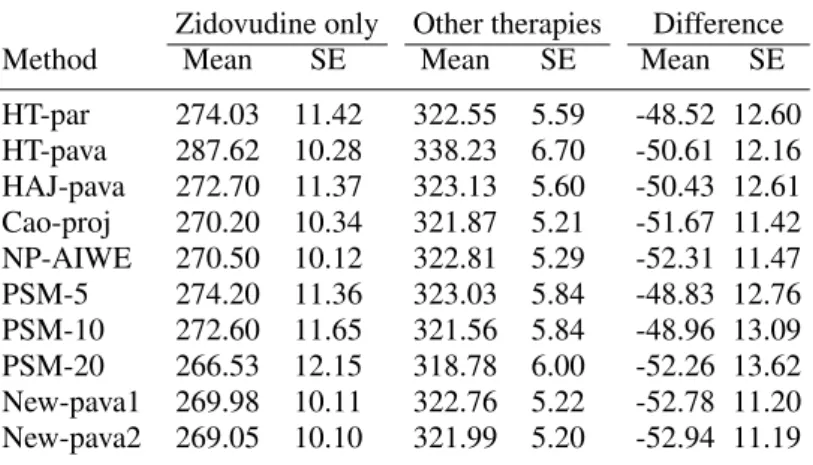
Table 4. Estimation of the marginal means of the CD4 T cell counts at week 96 in two groups, the zidovudine-only group and the other-therapy group, and estimation of the difference of the marginal means between these groups
Zidovudine only Other therapies Difference
Method Mean SE Mean SE Mean SE
HT-par 274.03 11.42 322.55 5.59 -48.52 12.60 HT-pava 287.62 10.28 338.23 6.70 -50.61 12.16 HAJ-pava 272.70 11.37 323.13 5.60 -50.43 12.61 Cao-proj 270.20 10.34 321.87 5.21 -51.67 11.42 NP-AIWE 270.50 10.12 322.81 5.29 -52.31 11.47 PSM-5 274.20 11.36 323.03 5.84 -48.83 12.76 PSM-10 272.60 11.65 321.56 5.84 -48.96 13.09 PSM-20 266.53 12.15 318.78 6.00 -52.26 13.62 New-pava1 269.98 10.11 322.76 5.22 -52.78 11.20 New-pava2 269.05 10.10 321.99 5.20 -52.94 11.19
4. The standard errors are obtained using 3000 bootstrap samples. The covariates listed above were included in the model for the propensity score of the missing probability and the working regression model of the response. Table4reports the estimates of the marginal means of the cell counts at week 96 in the two groups and the difference in the cell counts at week 96 between the groups.Cao-proj,NP-AIWE,New-pava1, andNew-pava2yield similar estimates and standard errors for the cell count differences, and the estimates differ from the estimates of the other methods. All the methods indicate that the marginal mean of the cell counts at week 96 is lower in the zidovudine group.
6. Concluding remarks
In causal inference and the missing data problem, the response mean is important. The statistical, economic, and epidemiological literature has many different estimation methods, such as the inverse probability weighting estimator ([12]) and the AIWE (Robins, Rotnitzky, and Zhao 1994). Other estimation methods such as propensity matching ([11]) are also available. For a comprehensive discussion of the related problems see the monograph by Imbens and Rubin [33]. It is well known that the propensity scoreπ(x)and the “working regression model” ψ(x)play extremely important roles in the mean estimation. In this paper we have provided a propensity score method that is almost nonparametric by using the monotonic single-index model. In contrast to doubly robust methods, where both the propensity score and the regression model have to be modeled as accurately as possible, our method requires us to model the regression model
ψ(x) =E(Y|X=x)carefully but leaves the propensity score almost nonparametric. It is encouraging that the inverse probability weighting estimators and AIWEs based on the nonparametrically fitted single-index model perform better than their counterparts based on the fitted correctly specified parametric model. To ease the computational burden in the semiparametric maximum likelihood estimation ofπ(x)for high-dimensional covariatesX, we propose first obtaining the estimateβbusing a “working parametric propensity score model,” say the logistic regression model. We can then estimate the link functionθ(·)using the PAVA based on the data(∆i, h(Xi)Tβb), i= 1,2, ..., n. We can successfully stabilize the
propensity score when it is too close to zero. Examples 2 and 3 showed that our method is more robust than the methods based on the fitted correctly specified parametric model. Further investigation of this method in regression parameter estimation based on missing data would be worthwhile.
Acknowledgements
The authors thank the editor, the associate editor, and the referee for constructive comments and suggestions that lead to a significant improvement over the article. Dr. Yu’s research is supported in part by Singapore Ministry Education Academic Research Fund Tier 1. Dr. Li was supported in part by the Natural Sciences and Engineering Research Council of Canada, RGPIN-2015-06592. Dr. Liu’s research is supported in part by National Institutes of Health grant, NIH P30 CA082709.
Appendix: Proofs of Theorems
Technical Conditions
We need the following conditions in the proof of Theorem 1.
Condition 1:Λ−1is a compact subspace ofRp−1.
Condition 2:There exists a constantC0independent ofusuch that
PI(β1τh(x)≤u)−I(β2τh(x)≤u)≤C0||β1−β2||1,
where∥ · ∥1denotes thel1norm.
Condition 3:θ0(·)∈Θandinfxθ0(v(x;β0))>0.
We need the following conditions in the proof of Theorem 2.
Condition A:The following technical conditions are for “π”:
A1:There exists0< α1<2such that for everyϵ >0,
H2,B(ϵ,F, FX)< A1ϵ−α1,
whereA1is a universal constant. A2:infπ∈Finfx|π(x)|>0.
A3:infxπ0(x)>0.
Condition B:The following technical conditions are for “ψ”:
B1:There exists0< α2<2such that for everyϵ >0,
H2,B(ϵ,Ψ, FX)< A2ϵ−α2,
whereA2is a universal constant. B2:supψ∈Ψsupx|ψ(x)|<∞.
B3:supxψ0(x)<∞.
Condition C:We further assume that the support offY(y)is bounded, wherefY(y)denotes the marginal density ofY.
Condition D:ψ0∈Ψ,infxw(1, x)>0, andsupδ,xw(δ, x)<∞.
Condition E:There exists a constantc >0such thatinfxθ(hT(x)β)> c >0.
Preliminaries
The proofs of the theorems rely heavily on empirical process theory. We adopt the usual notation in the literature. In particular, let “.” (“&”) denote smaller (greater) than, up to a universal constant. Recall thatPnandPare empirical and
probability measures, and for any functiong(v)and independent and identically distributed observationsV1, . . . ,Vn,
Pn(g(v)) = ∫ g(v)dPn = 1 n n ∑ i=1 g(Vi); P(g(v)) = ∫ g(v)dP.
Furthermore, we denote by∥g∥q,PtheLq normal ofgunderP. In particular,∥g∥q,P= {∫
gqdP}1/q.
We need the following definition of entropy for function classes, which plays a key role in modern empirical process theory. It is adapted from Definition 2.2 in van de Geer [28].
Definition 1 For anyϵ >0andq >0, letNq,B(ϵ,G,P)be the smallest value ofN for which there exists a set of pairs
of functions{(gL
j, gjU)}Nj=1 such that (i)∥gjU−gjL∥q,P≤ϵ, where∥gjU −gLj∥q,P= {∫
|gU
j −gjL|qdP }1/q
and (ii) for any
g∈ G, there exists aj=j(g)such that
gLj ≤g≤gUj.
Nq,B(ϵ,G,P)is called theϵ-bracketing number ofG, andHq,B(ϵ,G,P) = logNq,B(ϵ,G,P)is called theϵ-entropy with
Proof of Theorem 1
The proof of this theorem follows the same lines as part (a) of Theorem 1 in Chen et al. [22]; we omit it for brevity.
Proof of Theorem 2
To facilitate our proof, we need the following lemma, which is a direct application of Lemma 5.13 in van de Geer [28].
Lemma 1 Assume
sup
g∈G|
g−g0|∞≤1, H2,B(ϵ,G,P)≤Aϵ−α, (13)
for everyϵ >0and some0< α <2and some constantA. Then, for some constantcandn0depending onαandA, we
have for allT ≥candn≥n0,
P ( sup g∈G,∥g−g0∥2,P≤n−1/(2+α) Pn(g−g0)−P(g−g0)≥T n−2/(2+α) ) ≤cexp { −T nα/(2+α) c2 } (14) and P ( sup g∈G,∥g−g0∥2,P>n−1/(2+α) √ n|Pn(g−g0)−P(g−g0)| ∥g−g0∥ 1−α/2 2,P ≥T ) ≤cexp ( −T c2 ) . (15) We now prove Theorem 2. By (11) in the main text and straightforward manipulations, we immediately have
√ n(µbn−µ0)− √ nPnϕ(v, µ0, β0, π0(·), ψ0(·)) =√1 n n ∑ i=1 [{ 1 b π(Xi)− 1 π0(Xi) } ∆i{Yi−ψ0(Xi)} − { ∆i b π(Xi)− 1 }{ b ψ(Xi)−ψ0(Xi) }] =√nPnbg1(v)− √ nPnbg2(v), (16) wherebg1(v) = { 1 b π(x)− 1 π0(x) } δ{y−ψ0(x)},bg2(v) = { δ b π(x)−1 } { b ψ(x)−ψ0(x) } , andbg1∈ G1,bg2∈ G2with G1 = { g1(v) = { 1 π(x)− 1 π0(x) } δ{y−ψ0(x)}:π∈ F } G2 = { g2(v) = { δ π(x)−1 } {ψ(x)−ψ0(x)}:π∈ F;ψ∈Ψ } .
Using Conditions A–C, we can easily verify that
sup g1∈G1 |g1|∞.1, H2,B(ϵ,G1,P).ϵ−α1; (17) sup g2∈G2 |g2|∞.1, H2,B(ϵ,G2,P).ϵ−max{α1,α2}. (18)
With Lemma1, (17) implies that
P ( sup g1∈G1,∥g1∥2,P≤n−1/(2+α1 ) Png1−Pg1≥T n−2/(2+α1) ) ≤cexp { −T nα1/(2+α1) c2 } P ( sup g1∈G1,∥g1∥2,P>n−1/(2+α1 ) √ n|Png1−Pg1| ∥g1∥ 1−α1/2 2,P ≥T ) ≤cexp ( −T c2 ) . As a consequence, we have √ n|Pnbg1−Pbg1|=Op ( n− 2−α1 2(2+α1 ) ) ∨Op ( ∥bg1∥ 1−α1/2 2,P ) .
Herea∨b= max(a, b). With (18) and Lemma1, we similarly have
√ n|Pnbg2−Pbg2|=Op ( n− 2−max{α1,α2} 2(2+max{α1,α2}) ) ∨Op ( ∥bg2∥ 1−max{α1,α2}/2 2,P ) .
Noting thatα1<2andα2<2, andPbg1= 0, we immediately have √ n|Pnbg1| = Op ( ∥bg1∥ 1−α1/2 2,P ) +op(1), √ n|Pnbg2−Pbg2| = Op ( ∥bg2∥ 1−max{α1,α2}/2 2,P ) +op(1),
which, together with (16), Conditions A–C, and the fact that
Pbg2=P [{ π0(x) b π(x) −1 } { b ψ(x)−ψ0(x) }] ,
leads to (12) in the main text. This completes the proof of Theorem 2.
Proof of Corollary 1
By Theorem 2, (P1) immediately follows. Furthermore, by Theorem 2 and the conditions in (P2), we have
√
n(µb−µ0) =√nPnϕ(v;µ0, π0, ψ0) +op(1). (19)
Therefore, it remains to show thatµbachieves the information bound. By (19),ϕ(·;µ0, π0(·), ψ0(·))is the influence function.
Referring to the established theory for the semiparametric efficiency bound—e.g., Chapter 3 of Bickel et al. [34], Newey [35], Chapters 3 and 18 of Kosorok [30], and the references therein—we need to show only the following two parts:
(i) µbis a regular estimator ofµ0.
LetPηbe a submodel indexed byηsuch thatP0is the true model. Further, letµη=Eη(Y),πη(x) =Eη(∆|X =x),
andψη(x) =Eη(Y|X=x), whereEη indicates that the expectation is taken underPη. By Theorem 2.2 in Newey
[35], arguing thatbµis a regular estimator ofµ0is equivalent to showing that
∂µη ∂η η=0 =E0{ϕ(V;µ0, π0, ψ0)S0(V)}, (20) where S0(v) = ∂logfη(y, δ, x) ∂η η=0 ,
fη(y, δ, x)is the joint density of(Y,∆, X)underPη, andE0indicates that the expectation is taken under the true
distributionf0(y, δ, x).
(ii) There exists a submodelPη∗ withfη∗(y, δ, x)being the joint density of(Y,∆, X)underPη∗ such thatP0is the true
model and ϕ(v;µ0, π0, ψ0) = ∂logfη∗(y, δ, x) ∂η∗ η∗=0 .
We show Parts (i) and (ii) separately. To show Part (i), we need to verify (20). On the one hand,
µη=Eη(Y) = Eη{ψη(X)}, which leads to ∂µη ∂η η=0 =E0 { ∂ψη(X) ∂η η=0 } +E0{ψ0(X)S0(V)}. (21)
On the other hand,
E{ϕ(V;µ0, π0, ψ0)S0(V)}= ∂Eη{ϕ(V;µ0, π0, ψ0)} ∂η η=0 .
It can be verified that
Eη{ϕ(V;µ0, π0, ψ0)}=Eη [ {πη(X)−π0(X)}{ψη(X)−ψ0(X)} π0(X) +ψη(X) ] −µ0.
Note that{πη(X)−π0(X)}{ψη(X)−ψ0(X)}and its first derivative with respect toηare both equal to 0 atη= 0. Thus, E{ϕ(V;µ0, π0, ψ0)S0(V)}= ∂Eη{ϕ(V;µ0, π0, ψ0)} ∂η η=0 =E0 { ∂ψη(X) ∂η η=0 } +E0{ψ0(X)S0(V)},
which together with (21) implies (20). This proves Part (i).
We proceed to show Part (ii). LetfY|X;0(y|x)be the true conditional density ofY givenX =xandfX;0(·)the true
marginal density ofX. Consider
fη∗(y, δ, x) = [ 1 +η∗δ{y−ψ0(x)} π0(x) +η ∗{ψ 0(x)−µ0} ] fY|X;0(y|x){π0(x)}δ{1−π0(x)}1−δfX;0(x).
It is easy to check that for sufficiently smallη∗thisfη∗(y, δ, x)is a parametric submodel. The tangent of this submodel is
given by ∂logfη∗(y, δ, x) ∂η∗ η∗=0 = δ{y−ψ0(x)} π0(x) +ψ0(x)−µ0=ϕ(v;µ0, π0, ψ0),
which completes our proof of Part (ii). Therefore, we have completed the proof of this Corollary.
Proof of Theorem 3
Since we do not assume Condition A in this theorem, we first verify that Condition A is satisfied given Conditions 1–3 and B–E; then we prove the theorem by verifying the conditions in (P2) of Corollary 1. In fact, Conditions A2 and A3 are satisfied by reviewing Conditions 3 and E, so we need to verify only Condition A1. The following Lemma adapted from Lemma 2 of Chen et al. [22] ensures that Condition A1 is satisfied withα1= 1.
Lemma 2 Suppose Conditions 1 and 2 are satisfied. For anyϵ >0and integerq >0we have
Hq,B(ϵ,F, FX).1/ϵ,
whereF ={θ(hT(x)β) :θ∈Θ;β∈Λ}.
Therefore, to prove this theorem, we need to verify only that
∥bπ−π0∥2,P = op(1) (22) ∥ψb−ψ0∥2,P = op(1) (23) √ nP [{ π0(x) b π(x) −1 } { b ψ(x)−ψ0(x) }] = op(1). (24)
Note that (22) immediately follows by Theorem 1. Furthermore, by Conditions B and E, we have √nP [{ π0(x) b π(x) −1 } { b ψ(x)−ψ0(x)}].√n∥bπ−π0∥2,P∥ψb−ψ0∥2,P,
which together with Theorem 1 implies that both (23) and (24) hold if we can show that
∥ψb−ψ0∥2,P=oP(n−1/6). (25)
We proceed in two steps. First, note that Conditions D and E imply that
∥ψb−ψ0∥22,P.P [ w(1, x)π0(x){ψb(x)−ψ0(x)}2 ] =P [ w(δ, x){ψb(x)−ψ0(x)}2 ] . (26)
Second, by the definition ofψb, ifψ0∈Ψ, we haveQ(ψb)≤Q(ψ0).Hence, P[w(δ, x){ψb(x)−ψ0(x)}2 ] ≤ Q(ψ0)−Q(ψb) +P [ w(δ, x){ψb(x)−ψ0(x)}2 ] = Pn [ w(δ, x){y−ψ0(x)}2 ] −Pn [ w(δ, x){y−ψb(x)}2 ] +P [ w(δ, x){ψb(x)−ψ0(x)}2 ] = 2Pn [ w(δ, x){ψb(x)−ψ0(x)}{y−ψ0(x)} ] −(Pn−P) [ w(δ, x){ψb(x)−ψ0(x)}2 ] = 2Pnbg3−(Pn−P)bg4, (27)
wherebg3(δ, y, x) =w(δ, x){ψb(x)−ψ0(x)}{y−ψ0(x)} ∈ G3,bg4(δ, x) =w(δ, x){ψb(x)−ψ0(x)}2∈ G4, with G3 = {g3(v) =w(δ, x){ψ(x)−ψ0(x)}{y−ψ0(x)}:ψ∈Ψ},
G4 =
{
g4(v=w(δ, x){ψ(x)−ψ0(x)}2:ψ∈Ψ}.
By Conditions A–D, we can easily verify that
sup g3∈G3| g3|∞.1, H2,B(ϵ,G3,P).ϵ−α2; sup g4∈G4 |g4|∞.1, H2,B(ϵ,G4,P).ϵ−α2.
Therefore, Lemma1applies to bothG3andG4. That is,
P ( sup g3∈G3,∥g3∥2,P≤n−1/(2+α2 ) Png3−Pg3≥T n−2/(2+α2) ) ≤cexp { −T nα2/(2+α2) c2 } P ( sup g3∈G3,∥g3∥2,P>n−1/(2+α2 ) √ n|Png3−Pg3| ∥g3∥ 1−α2/2 2,P ≥T ) ≤cexp ( −T c2 ) and P ( sup g4∈G4,∥g4∥2,P≤n−1/(2+α2 ) Png4−Pg4≥T n−2/(2+α2) ) ≤cexp { −T nα2/(2+α2) c2 } P ( sup g4∈G4,∥g4∥2,P>n−1/(2+α2 ) √ n|Png4−Pg4| ∥g4∥ 1−α2/2 2,P ≥T ) ≤cexp ( −T c2 ) .
These together with the fact thatPbg3= 0lead to
|Pnbg3| = Op(n−2/(2+α2))∨ { n−1/2·Op(∥bg3∥ 1−α2/2 2,P ) } |(Pn−P)bg4| = Op(n−2/(2+α2))∨ { n−1/2·Op(∥bg4∥ 1−α2/2 2,P ) } . (28)
Furthermore, by Conditions B–D we have
∥gb3∥2,P.∥ψb−ψ0∥2,P, ∥bg4∥2,P.∥ψb−ψ0∥2,P. (29)
Combining (27)–(29), we immediately have
P[w(δ, x){ψb(x)−ψ0(x)}2 ] .Op(n−2/(2+α2))∨ { n−1/2·Op(∥ψb−ψ0∥ 1−α2/2 2,P ) } ,
which together with (26) and the condition that0< α2<2in Condition B leads to ∥ψb−ψ0∥2,P=OP(n−
1 2+α2).
This implies that (25) is correct, and this completes our proof.
References
1. Rubin D. Estimating causal effects of treatments in randomized and nonrandomized studies.Journal of Educational Psychology1974; 66: 688–701. 2. Rubin D. Direct and indirect causal effects via potential outcomes.Scandinavian Journal of Statistics2004; 31: 161–170.
3. Small DS, Joffe MM, Lynch KG, Roy JA, Localio AR. Tom Ten Haves contributions to causal inference and biostatistics: review and future research directions.Statistics in Medicine2014; 33: 3421-3433.
4. Burgess S, Small DS. Predicting the direction of causal effect based on an instrumental variable analysis: a cautionary tale.Journal of Causal Inference
2016; 4: 45-59.
5. Hahn J. On the role of propensity score in efficient semiparametric estimation of average treatment effects.Econometrica1998; 66: 315–332. 6. Mincer J.Schooling, Experience, and Earnings1974. New York: National Bureau of Economic Research.
7. Dehejia RH, Wahba S. Causal effects in nonexperimental studies: Reevaluating the evaluation of training programs.Journal of the American Statistical Association1999; 94: 1053–1062.
8. Lalonde RJ. Evaluating the econometric evaluations of training programs with experimental data.American Economic Review1986; 76: 604–620. 9. Graham BS, Pinto C, Egel D. Inverse Probability Tilting for Moment Condition Models With Missing Data.Review of Economic Studies2012; 79:
1052-1079.
10. Hastie TJ, Tibshirani RJ.Generalized Additive Models1990. Chapman & Hall/CRC.
11. Rosenbaum PR, Rubin DB. The central role of the propensity score in observational studies for causal effects.Biometrika1983; 70: 41-55.
12. Horvitz DG, Thompson DJ. A generalization of sampling without replacement from a finite universe.Journal of the American Statistical Association
1952; 47: 663–685.
13. Henmi M, Eguchi S. A paradox concerning nuisance parameters and projected estimating functions.Biometrika2004; 91: 929–941.
14. Robins JM, Rotnitzky A, Zhao LP. Estimation of regression coefficients when some regressors are not always observed.Journal of the American Statistical Association1994; 89: 846-866.
15. Scharfstein DO, Rotnitzky A, Robins JM. Adjusting for nonignorable drop-out using semiparametric nonresponse models (with discussion).Journal of the American Statistical Association1999;94: 1096–1120.
16. Wooldridge J. Inverse Probability Weighted Estimation for General Missing Data Problems.Journal of Econometrics2007; 141: 1281-1301. 17. Uysal SD. Doubly Robust Estimation of Causal Effects With Multivalued Treatments: An Application to the Returns to Schooling.Journal of Applied
Econometrics2015; 30: 763-786.
18. Sloczynski T, Wooldridge JM. A General Double Robustness Result for Estimating Average Treatment Effects 2014. IZA Discussion Paper 8084, Institute for the Study of Labor, Bonn, Germany.
19. Kang JD, Schafer JL. Demystifying double robustness: A comparison of alternative strategies for estimating a population mean from incomplete data (with discussion).Statistical Science2007; 22: 523–539.
20. Cheng PE. Nonparametric estimation of mean functionals with data missing at random.Journal of the American Statistical Association1994; 89: 81–87.
21. Cosslett SR. Distribution-free maximum likelihood estimator of the binary choice model.Econometrica1983; 51: 765–782.
22. Chen B, Li P, Qin J, Yu T. Using a monotonic density ratio model to find the asymptotically optimal combination of multiple diagnostic tests.Journal of the American Statistical Association2016; 111: 861-874.
23. Dykstra R, Kochar S, Robertson T. Inference for likelihood ratio ordering in the two-sample problem.Journal of the American Statistical Association
1995; 90: 1034–1040.
24. Ayer M, Brunk HD, Ewing GM, Reid WT, Silverman E. An empirical distribution function for sampling with incomplete information.The Annals of Mathematical Statistics1955; 26: 641–647.
25. R Development Core Team. R: A language and environment for statistical computing 2011. R Foundation for Statistical Computing, Vienna, Austria. URL: https://www.r-project.org/. ISBN: 3-900051-07-0.
26. Khan S, Tamer E. Irregular Identification, Support Conditions, and Inverse Weight Estimation.Econometrica2010; 78: 2021-2042.
27. Cao WH, Tsiatis AA, Davidian M. Improving efficiency and robutness of the doubly robust estimator for a population mean with incomplete data.
Biometrika2009;96: 723–734.
28. van de Geer SA.Empirical Processes in M-Estimation2000. Cambridge University Press, New York.
29. van der Vaart AW, Wellner JA.Weak Convergence and Empirical Processes with Applications to Statistics1996. Springer, New York. 30. Kosorok MR.Introduction to Empirical Processes and Semiparametric Inference2008. Springer, New York.
31. H´ajek J. Comment on “an essay on the logical foundations of survey sampling, part one.” In V. Godambe and D. Sprott (Eds.),Foundations of Statistical Inference1971. Toronto: Holt, Rinehart and Winston.
32. Hammer SM, Katzenstein DA, Hughes MD, Gundacker H, Schooley RT, Haubrich RH et al. A trial comparing nucleoside monotherapy with combination therapy in HIV-infected adults with CD4 cell counts from 200 to 500 per cubic millimeter. AIDS Clinical Trials Group Study 175 Study Team.New England Journal of Medicine1996; 335: 1081–1090.
33. Imbens GW, Rubin DB.Causal Inference for Statistics, Social, and Biomedical Sciences: An Introduction2015. Cambridge University Press, New York.
34. Bickel P, Klaassen CAJ, Ritov Y, Wellner JA.Efficient and Adaptive Estimation for Semiparametric Models1993. Johns Hopkins University Press, Baltimore.