UC Berkeley Previously Published Works
Title
Simulating multiple faceted variability in single cell RNA sequencing.
Permalink
https://escholarship.org/uc/item/3j1671ph
Journal
Nature Communications, 10(1)
Authors
Zhang, Xiuwei
Xu, Chenling
Yosef, Nir
Publication Date
2019-06-13
DOI
10.1038/s41467-019-10500-w
Peer reviewed
eScholarship.org
Powered by the California Digital Library
Simulating multiple faceted variability in single cell
RNA sequencing
Xiuwei Zhang
1,2,4, Chenling Xu
1,4& Nir Yosef
1,2,3The abundance of new computational methods for processing and interpreting tran-scriptomes at a single cell level raises the need for in silico platforms for evaluation and validation. Here, we present SymSim, a simulator that explicitly models the processes that give rise to data observed in single cell RNA-Seq experiments. The components of the SymSim pipeline pertain to the three primary sources of variation in single cell RNA-Seq data: noise intrinsic to the process of transcription, extrinsic variation indicative of different cell states (both discrete and continuous), and technical variation due to low sensitivity and measurement noise and bias. We demonstrate how SymSim can be used for benchmarking methods for clustering, differential expression and trajectory inference, and for examining the effects of various parameters on their performance. We also show how SymSim can be used to evaluate the number of cells required to detect a rare population under various scenarios.
https://doi.org/10.1038/s41467-019-10500-w OPEN
1Department of Electrical Engineering and Computer Sciences, Center for Computational Biology, UC Berkeley, Berkeley, CA 94720, USA.2Ragon Institute of Massachusetts General Hospital, MIT and Harvard, Cambridge, MA 02139, USA.3Chan-Zuckerberg Biohub, San Francisco, CA 94158, USA.4These authors
contributed equally: Xiuwei Zhang, Chenling Xu. Correspondence and requests for materials should be addressed to N.Y. (email:[email protected])
123456789
T
he advent of single cell RNA sequencing has led to a surge of computational and statistical methods for a range of analysis tasks. Some of the methods or the tasks that they perform have originated from bulk sequencing analysis, whileothers address opportunities (e.g., identification of new cell
states1,2) or technical limitations (e.g., limited sensitivity3,4) that
are idiosyncratic to single cell genomics5,6. While these
compu-tational methods are often based on reasonable assumptions it is
difficult to compare them to each other and assess their
perfor-mance without gold standards. One approach to address this is
through simulations7–12.
Existing simulation strategies (summarized by Zappia et al.13)
rely primarily on fitting distributional models to observed data
and then drawing from these distributions. While the resulting
models provide a goodfit to observed data, their parameters are
often abstract and do not directly correspond to the actual pro-cesses that gave rise to the observations. This leaves an important unaddressed problem in designing and using a simulator: the
need to modulate and then study the effects of specific aspects of
the underlying physical processes, such as the efficiency of mRNA
capture, the extent of amplification bias (e.g., by changing the
number of PCR cycles, or by using unique molecular identifiers
[UMI]), and the extent of transcriptional bursting. To address this, we present SymSim (Synthetic model of multiple variability factors for Simulation), a software for simulation of single cell RNA-Seq data. SymSim explicitly models three of the main
sources of variation that govern single cell expression patterns2:
allele intrinsic variation, extrinsic variation, and technical factors
(Fig. 1 and Supplementary Fig. 1). SymSim provides the users
with knobs to control various parameters at these three levels. First, we generate true numbers of molecules using a kinetic model, which allows us to adjust allele intrinsic variation and the extent of burst effect; second, we provide an intuitive interface to simulate a subpopulation structure, either discrete or along a
continuum, through specification of cluster-trees, which define a
low-dimensional manifold from which the transcriptional kinet-ics is determined for every gene and every cell; third, we simulate the main stages of the library preparation process and let users control the amount of variation stemming from these steps, such
as capture efficiency, amplification bias, varying sequencing
depth, and batch effect. Importantly, through this modeling scheme, SymSim recapitulates properties of the data (e.g., high abundance of zeros or increased noise in non-UMI protocols) without the need to explicitly force them as factors in a dis-tributional model.
We demonstrate the utility of SymSim in two types of
appli-cations. In thefirst example, we use it to evaluate the performance
of algorithms. We focus on the tasks of clustering, differential expression and trajectory inference, and test a number of meth-ods under different simulation settings of biological separability and technical noise. In the second example, we use SymSim for the purpose of experimental design, focusing on the question of how many cells should one sequence to identify a certain subpopulation.
Results
Allele intrinsic variation. The first knob for controlling the
simulation allows us to adjust the extent to which the infrequency of bursts of transcription adds variability to an otherwise homogenous population of cells. We use the widely accepted two-state kinetic model, in which the promoter switches between an
on and an off states with certain probabilities14,15. We use the
notationkonto represent the rate at which a gene becomes active,
koffthe rate of the gene becoming inactive,sthe transcription rate,
anddthe mRNA degradation rate. For simplicity, and following
previous work, wefixdto constant value of 114,16and consider
the other three parameters relative tod. Since RNA sequencing
Extrinsic variation Gene effects External variability
factors (EVF)
True transcript counts
Observed transcript counts KonKoffS KOn KOff Kinetic model Library preparation sequencing Intrinsic variation mRNA mRNA capturing Sequencing Read/UMI counts Fragmentation Amplification RT cDNA Single cells On Off S (synthesis) d (degradation) Technical variation
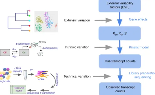
Fig. 1Overview of SymSim. The true transcript counts, which are the number of molecules for each transcript in each cell at the time of analysis, are generated through the classical promoter kinetic model with parameters: promoteronrate (kon),offrate (koff) and RNA synthesis rate (s). The values of the kinetic parameters are determined by the product of gene-specific coefficients (termed gene effects) and cell-specific coefficients. The latter set of coefficients is termed extrinsic variability factors (EVF), and it is indicative of the cell state. The expected value of each EVF is determined in accordance to the position of the cell in a user-defined tree structure. The tree dictates the structure of the resulting cell–cell similarity map (which can be either discrete or continuous) since the distance between any two cells in the tree is proportional to the expected distance between their EVF values. For homogenous populations (represented by a single location in the tree), the EVFs are drawniidfrom a distribution whose mean is the expected EVF value and variance is provided by the user. From the true transcript counts we explicitly simulate the key experimental steps of library preparation and sequencing, and obtain observed counts, which are read counts for full-length mRNA sequencing protocols, and UMI counts, otherwise
provides a single snapshot of the transcriptional process, we resort to assuming that the cells are at a steady state, and thus that the resulting single-cell measurements are drawn from the
sta-tionary distribution of the two-state kinetic model. Since d is
fixed, we are able to express the stationary distribution for each
gene analytically using a Beta-Poisson mixture17(Methods).
The values of the kinetic parameters (kon,koff, ands) for each
gene in each cell are first calculated using a product of
cell-specific and gene-specific factors, then adjusted by the parameter
distributions estimated from experimental data (Fig. 2a,
Meth-ods). Specifically, each cell is assigned with three low-dimensional
vectors (in this section, we used dimension 10; different values can be set by the user), one for each kinetic parameter. Similarly, each gene is associated with three low-dimensional vectors of the same dimension, which we term gene effect vectors. The value of each parameter is determined by the dot product of the two
respective vectors (Fig.2a).
The coordinates of a cell’s vectors represent factors of cell to
cell variability that are extrinsic to the noise generated intrinsically by the process of transcription (which we model by drawing from the stationary distribution above). These values, which we term extrinsic variability factors (EVF) represent a low dimension manifold on which the cells lie and can be interpreted as concentrations of key proteins, morpho-logical properties, microenvironment and more. When simulat-ing a homogeneous population, the EVFs of the cells are drawn
from a normal distribution with a fixed mean of 1 and a
standard deviation σ. σ is the within-population variability
parameter and can be set by the user (for the results in this
sectionσis set to 0.5).
The coordinates of the gene effect vectors can be interpreted as the dependence of its kinetics on the levels of EVFs. For instance, a positive value means that higher concentration of the
corresponding EVF can give rise to a higher onrate of a certain
promoter (if the EVF and gene effect vectors are both for
parameter kon). The gene effect values are first drawn
indepen-dently from a standard normal distribution. We then replace each
gene effect with a value of zero with probabilityη, thus ensuring
that every gene is only affected by a small subset of EVFs. The
sparseness parameterηcan be set by the user; in this paper we set
it to afixed value of 0.7.
To map the values of kinetic parameters calculated as dot product of the EVF and gene effect vectors into realistic ranges,
wefirst estimate the distribution of kinetic parameters of genes
from real data byfitting a Beta-Poisson model (Methods). To gain
a robust estimation of the distribution of kinetic parameters to be used by SymSim, we performed the estimation multiple times with (1) different subpopulations of a dataset; (2) different
imputation methods (scVI4 and MAGIC18) to reduce technical
variation in real data. Then we obtain aggregated distributions
from the results of all the settings we considered (Fig. 2b,
Methods, sources of real data described in Data Availability). Notably, the goal of performing kinetic parameters estimation from real data is mainly to identify the range of plausible parameter values to scale the dot products. The ranges in the
distributions we obtain (Fig. 2b) are in line with observations
from other experiments19–27 (Supplementary Note 1,
Supple-mentary Table 1). SymSim then applies a quantile approach to map the simulated parameter values resulting from the dot
products into the aggregated distributions (Fig.2a, Methods).
Finally, we account for the possibility of outlier genes with unusually high-expression level, commonly observed in real data. These outlier genes are hard to model with distributional
methods, and require additional parametrization13. This
phenomena is more pronounced in datasets from certain
protocols (for example, 10x Chromium28) than others (for
example, Smart-seq229), possibly due to selection bias which
can be exacerbated by low capture rate. In SymSim, we model the high-expression outlier genes by designating a small subset of genes (whose proportion is determined by the parameter prop_hge) as constitutively transcribed, and adjusting their
transcription rate s by a factor determined by the parameter
mean_hge(>1; Methods).
An intriguing question in the analysis of single cell RNA-seq data is the extent to which the conclusion drawn from the data
(e.g., stratification into subpopulations) may be confounded by
transcriptional bursting and transcriptional noise. SymSim
provides a way to explore this. We first note that modality15,17
and extent of the intrinsic noise15in the expression of a gene in a
homogenous population of cells (i.e., cells with similar EVFs) can
vary for the different ranges of kon, koff, ands. Specifically, one
can distinguish the following three types of gene-expression
distributions by the number of inflection points in the smoothed
density function: unimodal with highest frequency at 0 (no
inflection point), unimodal with highest frequency at non-zero
value (one inflection point), and bimodal (two inflection points).
Figure 2c shows the number of inflection points for different
configurations ofkonandkoffwith givens=10. This gives a clear
correspondence between kinetic parameter configurations and
types of gene-expression distributions. For example, when s is
relatively large, we obtain bimodal distributions whenkonandkoff
are smaller than 1.
These results thus guide us in tuning kinetic parameters to obtain desired gene-expression distributions to simulate.
Speci-fically, we focus on adjustment of the bimodality of the
distribution, which can lead to large, yet transient fluctuations
in mRNA concentration at the same cell over time, thus potentially misleading methods for cell state annotation and differential expression. To increase the overall extent of
bimodality in the data, we divide (decrease) all kon and koff
values by 10bimod (Fig.2c, yellow arrow). The parameterbimod
can take value from 0 to 1. This way, other properties such as
burst frequency (kon/(kon+koff)) and synthesis rate (s) remain the
same. In Fig. 2d we show the effect of varying the bimod
parameter on gene-expression distribution in a simulated
homogenous population. Expectedly, asbimodincreases, so does
the number of bimodal genes, as well as the average Fano factor (Supplementary Fig. 2a).
Extrinsic variation via extrinsic variability factors. While the
first knob focuses on variation within a homogeneous set of cells,
the second knob allows the user to simulate multiple, different cell states. This added complexity is achieved by setting different EVF values for different cells, in a way that allows users to control cellular heterogeneity and generate discrete subpopulations or continuous trajectories. To this end, SymSim represents the
desired structure of cell states using a tree (which can be specified
by the user), where every subpopulation (in the discrete mode) or every cell (in the continuous mode) is assigned with a position along the tree. Different positions in the tree correspond to dif-ferent expected EVF values, and the expected absolute difference between the value of an EVF of any two cells is linearly pro-portional to the square root of their distance in the tree (Sup-plementary Notes 2 and 7).
When SymSim is applied in a discrete mode, the cells are sampled from the leaves of the tree. The set of cells that are assigned to the same leaf in the tree form a subpopulation, and their EVF values are drawn from the same distribution. As above, we draw these EVF from a normal distribution, where the mean is determined by the position in the tree and the standard deviation
a c b Density d log 10 (K of f )
log10(Koff) log10(s)
log10(Kon)
log10(Kon)
Bimod = 0
Genes
Bimod = 0.4 Bimod = 1
Log10 count bins 0.0 (0,0.4](0.4,0.8] (0.8,1.2](1.2,1.6](1.6,2](2,2.4](2.4,2.8](2.8,3.2](3.2,3.6](3.6,4] 0.0 (0,0.4](0.4,0.8] (0.8,1.2](1.2,1.6](1.6,2](2,2.4](2.4,2.8](2.8,3.2](3.2,3.6](3.6,4] 0.0 (0,0.4](0.4,0.8] (0.8,1.2](1.2,1.6](1.6,2](2,2.4](2.4,2.8](2.8,3.2](3.2,3.6](3.6,4] Log10 count bins
Log10 count bins Map dot products K’on, K’off, S’ to distributions from real data
and get “matched parameters” Kon, Koff, S
*
n: # cells p: # of EVFs Koff Kon S d G1,1 G1,p Gm,p Gm,1 Kongene effect*
G1,1 G1,p Gm,p Gm,1*
G1,1 G1,p Gm,p Gm,1=
=
=
E1,1 E1,n Ep,1 Ep,n E1,1 E1,n Ep,1 Ep,n E1,1 E1,n Ep,1 Ep,n Kon 1,1 K on 1,n Kon m,1 K on m,n Koff 1,1 K off 1,n Koff m,1 Koffm,n m: # genes S1,1 S1,n Sm,1 Sm,n S’Sample transcript counts
0.04 0.03 0.02 0.01 0.00 –1 0 1 2 –1 0 1 2 1 2 3 2 1 0 –1 –2 –2 –1 0 1 2
Number of modes in transcript distribution
One mode at zero One mode at non-zero value Two modes KonEVF KoffEVF S EVF K′on K′off Koffgene effect S gene effect 0.04 0.05 0.04 0.04 0.02 0.00 0.03 0.02 0.01 0.00 0.05 0.04 0.04 0.02 0.00 0.03 0.02 0.01 0.00 0.03 0.02 0.01 0.00 –1012 –1012 1 2 3 Freq 0.75 0.50 0.25 0.00
Fig. 2Intrinsic variation.aA diagram of how gene and cell-specific kinetic parameters are simulated from cell-specific EVF and gene-specific gene effect vectors, and how the kinetic parameters are used in a model of transcription. Each cell has a separate EVF vector forKon,Koff, andS. Each parameter is generated through two steps:first, for each gene in each cell, we take the dot product of the corresponding EVF and gene effect vectors. Second, the dot product values are mapped to distributions of parameters estimated from experimental data. The matched parameters are used to generate true transcript counts (see Methods).bThe distributions ofkon, koff, andsthat are used in SymSim for simulations. These distributions are aggregated from inferred results of three subpopulations of the UMI cortex dataset (oligodendrocytes, pyramidal CA1 and pyramidal S1) after imputation by scVI and MAGIC.
cA heatmap showing the effect of parameterkonandkoffon the number of modes in transcript counts. The value of s isfixed to 10 in this plot. The red area with lowkonandkoffhave one zero mode and one non-zero mode. The gray area with lowkonand highkoffhas only one zero mode, and the blue area with highkonand lowkoffhave one non-zero mode. The yellow arrow shows how the parameterbimodcan modify the amount of bimodality in the transcript count distribution.dHistogram heatmaps of transcript count distribution of the true simulated counts with varying values ofbimod, showing that increasing
bimodincreases the zero-components of transcript counts and the number of bimodal genes. In these heatmaps, each row corresponds to a gene, each column corresponds to a level of expression, and the color intensity is proportional to the number of cells that express the respective gene at the respective expression level. Data used to plotb–dcan be found in Source Data
continuous mode, the cells are positioned along the edges of the tree with a small step size (which is determined by branch lengths and number of cells; Methods). The EVF values are then drawn from a normal distribution where the mean is determined by the
position in the tree, and the standard deviation is defined by σ
(Fig.3a).
To facilitate the correspondence between EVF values and distances in the tree we use a Brownian motion procedure as
described in ref.30(Methods; Fig.3a). Specifically, for each EVF
we set the mean value at the root of the tree to afixed number
(default set root node to 1) and then perform Brownian motion
along the branch. Fig.3a illustrates this process using populations
2 and 3 in the tree as an example. Notably, in the continuous mode, this formulation can give rise to a rich set of patterns of changes in gene expression from root (progenitor cells) to leaves (target cells), including the commonly observed impulse
profile31,32(Supplementary Fig. 3c–d). As an alternative, we also
implemented a mode for simulating continuous data by which gene expression from root to leaves is determined explicitly by an impulse function. This might be preferable if the user would like
to generate smoother changes in gene expression, or specific
temporal patterns. In the following analyses we use the Brownian motion model.
Notably, SymSim only generates a subset of EVFs from the tree, while the remaining ones are drawn from the same
distribution for all subpopulations (Fig. 3a). The tree-sampled
subset, which we term Diff-EVFs (Differential EVFs) represents
the conditions or factors which are different between subpopula-tions, and they usually account for a small proportion of all the EVFs. The number of Diff-EVFs can be set by the user. The results in this section were produced with 60 EVFs, 20% of them are Diff-EVFs.
With this formulation, users can control the extent of between-population variation by setting the branch lengths of the input tree, and combine it with a desired level of within-population
variation by setting the parameter σ. Notably, both σ and the
square root of branch lengths in the tree are in units of EVF values. It is therefore the case that for any two positions in the
tree, the ratio of square root tree distance to σdetermines the
separability between the respective distributions of the values assigned to any given Diff-EVF (Supplementary Note 2). As
illustration, Fig.3depicts the tSNE plots of cells from the same
input tree with different σ in either a discrete (Fig. 3b) or
continuous (Fig. 3c) mode. Notably, both panels show that the
tSNE plots reflect the structure of the input tree well.
Technical variation. The third knob of SymSim allows users to
control technical variation, which accounts for a large part of the
variation observed in scRNA-seq datasets33–35. The technical
confounders reflect noise, reduced sensitivity and bias that are
introduced during sample processing steps such as mRNA
cap-ture, reverse transcription, PCR amplification, RNA
fragmenta-tion, and sequencing. In order to introduce realistic technical variation into our model, we explicitly simulate the major steps in
a
pop2 pop3 pop4 pop5 pop1
Diff-EVFs Non Diff-EVFs y3(1) Node6 Node7 y2(1) Node8 Tips b c 1 6 Diff-EVF mean 2 1 0 –1 7 8 9 4 5 1 3 2 1 1 0.2 0.2 1 1 3 N(1, σ2) N(1, σ2) N(1, σ2) N(1, σ2) N(1, σ2 ) N(1, σ2) N(y2(1), σ2) N(y 3(1), σ 2) N(y 3(2), σ 2) N(y2(2), σ2 ) tSNE1 –10 –10 –5 0 5 –10 0 10 20 –10 –5 0 5 10 15 20 10 5 0 –5 10 10 0 0 –10 –10 –20 10 0 –10 0 10
tSNE1 tSNE1 tSNE1
tSNE2
tSNE2
σ = 0.4 σ = 0.7 σ = 0.4 σ = 0.7
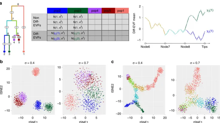
Fig. 3Extrinsic variation.aIllustration of generating a diverse set of cell states with SymSim. The tree represents the relationship between cells. The numbers on the edges are branch lengths; the node numbers indicate the ID of the respective subpopulation (each subpopulation is represented by a single position [leaf] in the tree). The matrix to the right depicts the derivation of EVF values. Each row corresponds to an EVF (only two are Diff-EVF), each column corresponds to a position in the tree, and the content specifies the distribution from which the EVF values are drawn. We use the notationya(b)to represent the expected value of EVFbin positionain the tree. The rightmost plot depicts the derivation of these expected values with Brownian motion. We use subpopulations 2 and 3 as examples for both discrete cases (sampling only cells within the subpopulations) or continuous (sampling cells along the trajectories from the root progenitor state [node 6] to the two target subpopulations [nodes 2 and 3]).btSNE plots offive discrete populations generated from the tree structure shown ina. Different values ofσgive rise to different heterogeneity of each population.ctSNE plots of continuous populations generated from the same tree. The colors correspond to the colors on branches in the tree shown ina. When increasingσ, cells are more scattered around the main paths which follow the tree structure. Data used to plotb, ccan be found in Source Data
the experimental procedures. We implemented two library
pre-paration protocols: (1) full-length mRNAs profiling without the
use of UMIs (e.g., with a standard SmartSeq229); and (2) profiling
only the end of the mRNA molecule with addition of UMIs (e.g.,
10x Chromium28). The former protocol is usually applied for a
small number of cells and with a large number of reads per cell,
providing full information on transcript structure36. The latter is
normally applied for many cells with shallower sequencing, and it
is affected less by amplification and gene length biases33.
The workflow of these steps is shown in Fig. 4a (Methods).
Starting from the simulated true mRNA content of a given cell (namely, number of transcripts per gene, sampled from the
stationary distribution of the promoter kinetic model), the first
step is mRNA capture, where every molecule is retained with
probability^α. The value of the capture efficiency^αassociated with
each cell is drawn from a normal distribution with a meanαand
standard deviation β, which can be set by the user. The second
step is amplification, where in every cycle SymSim selects each
a
Simulated observed log counts
Simulated true log counts
NonUMI UMI High quality 15 15 10 5 0 10 5 0 10 5 0 5 0 10 0 5 10 5 0 10 0 5 10 10 5 0 Low quality
High quality Low quality
d e
log10(mean+1) Percent nonzero log10(sd)
b c Experimental Simulated Log2(mean(TPM)) Log2(gene length) Simulation by SymSim
Experimental UMI cortex
NonUMI UMI 10x t4k UMI cortex nonUMI UMI 10x t4k 1.00 4 3 2 2 1 0 –1 –1 0 1 –1 0 1 –1 0 1 2 1 0 2 0.75 Freq 0.50 0.26 0.00 1 0 2.0 1.5 1.0 0.5 0.0 0 1 2 0 1 2 3 4 0.00 0.25 0.50 0.75 1.00 0.00 0.0 0.5 1.0 1.5 2.0 0.25 0.50 0.75 1.00 0.00 0.25 0.50 0.75 1.00 0 1 2 3 4 0.75 4 2 0 0.50 0.25 1.00 0.75 0.50 0.25 0.00 1.00 0.75 0.50 0.25 0.00 Non-UMI 10.0 True count = 16 Transcript capture efficiency
CEL-seq linear amplification Pre-amplification: 1st round of PCR Nth round of PCR Fragmentation
Another k rounds of PCR amplification
Sequencing 1 1 2 0 2 0 0 0 2 0 2 2 0 0 0 c1 0 c2 0 0 0 c3 0 c4 c5 0 0 c6 c7c8 0 2 2 2 0 1 0 0 0 1 1 1 1 0 0 1 1 1 0 1 1 1 1 1 1 1 1 1 1 1 1 1 1 1 2n 0 2n 2n 2n 2n 2n 0 0 0 0 0 0 0 0 0 0 0 0 0 0 0 0 0 0 0 0 0 0 0 0 0 0 0 0 0 0 0 0 0 0 0 0 0 0 0 x12 k y1 y2 y3 y4 y5 y6 x22 k x32 k x42 kx52 k x62 k x1 x2 x3 x4 x5 x6 7.5 5.0 2.5 0.0 9 10 11 12 13 9 10 11 12 13 10.0 7.5 5.0 2.5 0.0 True counts, simulated 6 k = 1 UMI count = Σ (I(Yi > 0)) 6 k = 1 Read count = ΣYi Observed counts, simulated Observed counts, experimental 0.0 (0,0.4](0.4,0.8](0.8,1.2](1.2,1.6](1.6,2](2,2.4](2.4,2.8](2.8,3.2](3.2,3.6](3.6,4] 0.0 (0,0.4](0.4,0.8](0.8,1.2](1.2,1.6](1.6,2](2,2.4](2.4,2.8](2.8,3.2](3.2,3.6](3.6,4] 0.0 (0,0.4](0.4,0.8](0.8,1.2](1.2,1.6](1.6,2](2,2.4](2.4,2.8](2.8,3.2](3.2,3.6](3.6,4]
log10(count) bins log10(count) bins log10(count) bins
...
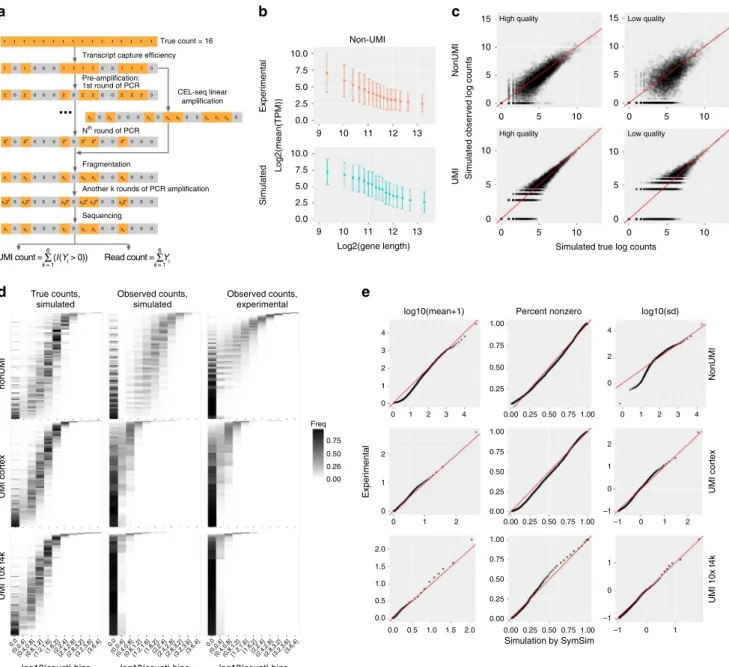
Fig. 4Technical variation.aA diagram showing the workflow of adding technical variation to true simulated counts. Each gray or orange square represents a molecule of the same transcript in one cell. We implement the following steps: mRNA capturing, pre-amplification (PCR or linear amplification of the cDNAs), fragmentation, amplification after fragmentation, sequencing, and calculation of UMI counts or read counts. Details of these steps can be found in Methods.bGene length bias in both simulated and experimental data for the non-UMI protocol. Error bars represent the ranges of (mean-SD, mean+SD), where SD means standard deviation.cScatter plots comparing true counts and observed counts obtained through: (1) non-UMI, good parameters (α=0.2,
MaxAmpBias=0.1,Depth=1e6) for high quality data; (2) UMI, good parameters (α=0.2,MaxAmpBias=0.1,Depth=5e5) for high quality data; (3) non-UMI, bad parameters (α=0.05,MaxAmpBias=0.2,Depth=1e6) for low quality data; (4) UMI, bad parameters (α=0.04,MaxAmpBias=0.2,Depth=
5e5) for low quality data.d2D transcript counts histogram heatmap of UMI and non-UMI simulated true counts and simulated observed counts, generated with parameters which best match the input experimental counts, and histogram heatmaps of the respective experimental counts (non-UMI Th17, UMI cortex and UMI 10x t4k datasets).eQ–Q plots comparing the mean, percent non-zero and standard deviation in experimental counts and SymSim simulated observed counts respectively for the non-UMI, UMI cortex and UMI 10x t4k datasets. A good match is indicated by most of the dots falling close to the red line. Data used to plotb–ecan be found in Source Data
available molecule with a certain probability and duplicates it.
The expected amplification efficiency and the number of PCR
cycles can be set by the user. As an optional step, SymSim
provides the option of linear amplification (e.g., as in CEL-Seq37).
We do not apply this option in this manuscript. In the third step
each amplified molecule is broken down into fragments, in
preparation for further amplification, size selection, and
sequen-cing (Methods).
The number of reads per cell (namely, the number of sequenced fragments) is drawn from a normal distribution whose
mean is determined by the parameterDepth, which, along with
the respective standard deviation (Depth_sd) can be provided by
the user. To derive thefinal observed expression values we do not
account for sequencing errors, and assume that every sequenced fragment is assigned to the correct gene it originates from. For the
non-UMI option, we define the raw measurement of expression
as the number of reads per gene. If UMIs are used, SymSim counts every original mRNA molecule only once by collapsing all reads that originated from the same molecule. Notably, for certain depth values, the resulting distribution of number of reads per UMI is similar to the one observed in a dataset of murine cortex
cells38(Supplementary Fig. 4a, Supplementary Fig. 1G of the cited
paper).
It has been previously shown that estimation of gene-expression levels from full-length mRNA sequencing protocols
has amplification biases related to sequence-specific properties
like gene length and GC-content33,39, whereas the use of UMIs
can correct these biases39,40. In particular, we have observed a
negative correlation between gene length and length-normalized gene-expression in our reference non-UMI dataset (murine Th17
cells from Gaublomme et al.41; Fig.4b), and the same trend is
reported by Phipson et al.39. To account for that, we parametrize
the efficiency of the PCR amplification step using a linear model
that represents gene length bias (Methods). As a result, our simulated data with a non-UMI protocol show a similar dependence of gene-expression on gene length as in experimental
data (Fig.4b, real data is from ref.41). In cases where UMIs are
used, gene length effects are also modeled during amplification,
but these effects are mitigated since each molecule is counted at most once. We therefore do not observe gene length bias in the UMI-based simulated data, similarly to the experimental data
(Supplementary Fig. 4b, real data is from ref. 38). Finally, we
model batch effects with multiplicative factors that are gene- and
batch-specific. In Supplementary Fig. 4c, we show the same
population of cells are separated by batches. To simplify the discussion at the remainder of this paper, we assume that the data come from a single batch.
In Fig.4c, we show the comparison between the simulated true
mRNA content of one cell and the simulated observed counts obtained with or without UMI. We consider two scenarios: the
first scenario represents a study with a low technical confounding
and the second one represents a highly confounded dataset.
Parameters which differ between these“good”and“bad”cases in
this example include capture efficiency (α), extent of amplifi
ca-tion bias (MaxAmpBias), and sequencing depth (Depth). Using
“bad”technical parameters introduce more noise to true counts,
and compared to the non-UMI simulation the UMIs reduce technical noise. The histograms of true counts and four versions of simulated counts are shown in Supplementary Fig. 4d. Using
quantile-quantile plots (Q–Q plots; Supplementary Fig. 4e)
further demonstrates that UMIs help in maintaining a better representation of the true counts in the observed data.
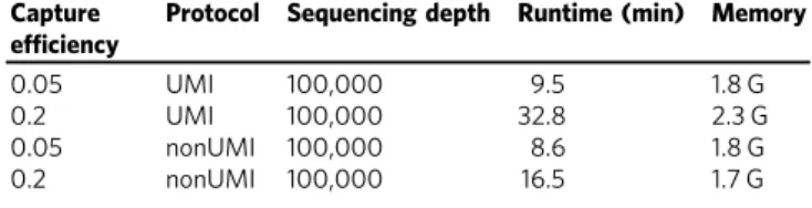
The total computation time to simulate a dataset consists of time to generate true counts and time to generate observed counts from true counts. We show the runtime and memory usage for
different parameter configurations in Methods.
Fitting parameters to real data. For a given real dataset, SymSim
can produce observed (read or UMI) counts that have similar
statistical properties to the real data (Fig.4d–e), by searching in a
database of simulations obtained from a range of parameter
configurations (Methods). This procedure focuses on
within-population variability (similarly to Splatter13) and sets the values
of ten parameters from both thefirst and third knobs (Methods).
We test this function with the non-UMI Th17 dataset41(using all
cells), the UMI cortex dataset38 (using a subpopulation of 948
CA1 pyramidal neuron cells) and two UMI datasets from 10x
Genomics, denoted by “UMI 10x t4k”and “UMI 10x pbmc8k”
(details and sources of experimental data are described in Data Availability). See Supplementary Note 4 and Supplementary
Tables 2–5 for the values of thefitted parameters.
Side by side inspection of the histograms of true mRNA levels (simulated) and observed counts (simulated and experimental), indicates that SymSim can transform the simulated ground truth
(Fig.4d, left) into simulated observations (Fig. 4d, middle) that
match the real observed data for both UMI and non-UMI
protocols (Fig. 4d, right). For a more quantitative analysis, we
generated Q–Q plots of the distributions of mean (after adding
one to all values), percent non-zero and standard deviation (SD)
of genes between simulated and experimental data (Fig. 4e,
Supplementary Fig. 5b for the UMI 10x pbmc8k dataset). Notably, we observe a certain level of inaccuracy in matching the SD at the lower ends for the non-UMI data, which can be due to lowly expressed genes. Indeed, when we exclude lowly expressed genes from the real data, the matching of SD improve
substantially (Q–Q plots shown in Supplementary Fig. 5a).
Furthermore, we conducted a similar analysis by training
Splatter13 and powSimR12 with the same experimental datasets
as input, and found that SymSim matches this data significantly
better (Supplementary Fig. 5c). Q–Q plots of the distributions of
coefficient of variation (CV) and mean (without adding one) of
genes between experimental data and data simulated, respectively, by SymSim, Splatter and powSimR also show that SymSim
provides an overall better fit than the other two simulators
(Supplementary Fig. 5d–e). We also performed additional
comparisons of the simulators with other measurements, described in Supplementary Note 5 and shown in Supplementary
Figs. 6a–b and 7a–c.
Comparing computational methods for single cell RNA-seq
data. SymSim can be used to benchmark methods for single cell
RNA-Seq data analysis as it provides both observed counts and a reference ground truth. In the following sections we demonstrate the utility of SymSim as tool for benchmarking methods for clustering, differential expression, and trajectory inference in a sample consisting of multiple subpopulations, using the structure
depicted in Fig.3a. The design of SymSim allows us to evaluate
the effect of various biological and technical confounders on the accuracy of downstream analysis. Here, we investigate the effect
of total number of cells (N), within population variability (σ),
mRNA capture rate (α), and sequencing depth (Depth). We also
test the effect of the proportion of cells associated with the
smallest subpopulation of cells (Prop), using population 2 in the
tree as our designated rare subpopulation.
Using SymSim to evaluate clustering methods. We begin by
inspecting the impact of each parameter on the performance of clustering methods. To this end, we simulated observed counts
using the UMI option, and traversed a grid of values for thefive
parameters with 18 simulation runs per configuration. The values
of the remaining parameters are largely determined according to
tested three clustering methods: k-means based on Euclidean
distance of thefirst 10 principle components, k-means based on
Euclidean distance in a nonlinear latent space learned by scVI4
and SIMLR42. In all cases we set the expected number of clusters
to the ground truth value (k=5). The accuracy of the methods is
evaluated using the adjusted Rand index (ARI; higher values indicate better performance). To inspect the effects of the various parameters on clustering performance, we performed multiple linear regression between the parameters and the ARI. The
regression coefficients are shown in Fig.5a. Overall,σappears to
be the most dominant factor, and the proportion of the rare
population (Prop) is clearly positively associated with better
performance. Among the technical parameters, while α plays a
role on the performance especially for the rare population, the
impact ofDepthis minor.
We then focus on varying the dominant factors (except N,
which we discuss in the next section), namely, the
within-population variation parameterσand mRNA capture efficiencyα,
for the benchmarking analysis henceforth. In particular, the range
of values for σ is set such that we cover various data
characteristics, from well separated populations, to almost entirely mixed ones (Supplementary Table 6). We compare the
performance of four clustering strategies: SIMLR42,
dimension-ality reduction with scVI4followed by k-means, and
dimension-ality reduction with PCA followed by Louvain clustering43
(implemented in Seurat44) or k-means. We observe better
accuracy as the quality of the data increases or the
within-population variation decreases (Fig.5b–c). Interestingly,
compar-ing σ=0.6, σ=0.8, andσ=1, we can tell that whenσ is high
enough to make the clustering challenging, further increasing σ
does not yield obvious changes (Fig. 5b). We observe a similar
trend of saturation, inspecting increasing levels of capture
efficiency (α), especially with scVI. Comparing the methods to
each other, we see that scVI/k-means has the highest ARI in most cases; when the rare population accounts for 5% of all cells, Seurat is the second best and PCA/k-means and SIMLR are comparable; when the rare population accounts for 10% of all cells, SIMLR performs slightly worse than Seurat and PCA/k-means.
0.05 0.04 0.00 –0.04 1.0 0.9 0.8 0.7 Average over all populations
a b c Prop = 5% Prop = 5% Prop = 10% Prop = 10% Rare population PCA+kmeans scVI+kmeans SIMLR PCA+kmeans scVI+kmeans SIMLR PCA+Louvain (Seurat) Method 0.00 Coefficients Adjusted r a nd inde x Adjusted r a nd inde x –0.05 –0.10 1.0 0.9 0.8 0.7 0.6 1.0 0.8 0.6 0.4 1.0 0.8 0.6 0.4 Depth 0.4 0.001 0.005 0.01 0.025 0.04 0.1 0.2 0.6 0.8 1 N Prop σ σ 0.4 0.6 0.8 1 σ α α 0.001 0.005 0.01 0.025 0.04 0.1 0.2 α Depth N Prop σ α
Fig. 5Benchmarking of clustering methods.aCoefficients of various parameters from multiple linear regression between parameters and the adjusted Rand index (ARI). In the left plot the ARI are averaged over all populations, and in the right plot the ARI is only for the rare population (population 2).bARI of the rare populations using the four clustering methods when changingσ(α=0.04). Left plot: the rare population accounts for 5% of all the cells; right plot: the rare population accounts for 10% of all the cells.cARI of the rare populations using the four clustering methods when changingα(σ=0.6). Left plot: the rare population accounts for 5% of all the cells; right plot: the rare population accounts for 10% of all the cells. Data used to plota–ccan be found in Source Data
Using SymSim to evaluate differential expression methods. Our mechanism for simulating multiple populations automatically generates differentially expressed (DE) genes between
popula-tions (in the discrete setting; Fig. 3b) or along pseudotime (in
the continuous setting; Fig.3c). In the following, we use SymSim
to benchmark methods for detecting DE genes, focusing on the
discrete setting. We use two criteria to define the ground truth
set of DE genes. Thefirst criterion is that the number of
Diff-EVFs that are associated with a non-zero gene effect value
(which we denote as nDiff-EVFgene; Fig. 6a) should be larger
than zero. This criterion is motivated by our model of tran-scription regulation: the kinetic parameters of a gene are affected by extrinsic factors, and changes to extrinsic factors might
therefore lead to changes in the number of transcripts. Indeed, when we compare the true simulated gene expression values between subpopulations (i.e., before introducing technical con-founders), we get a uniform (random) distribution of p-values for genes with no Diff-EVFs, and an increasing skew as
nDiff-EVFgene increases (Fig.6b, using Wilcoxon test);
Supplemen-tary Fig. 9a shows that the log fold change of gene-expression between subpopulations increases with nDiff-EVFgene. An additional constraint for a gene being differentially expressed is
that it must have a sufficiently large fold change in their
simulated true simulated expression levels (threshold of absolute log2 fold change ranges from 0.6 to 1, details in Figure legends; Methods).
a
Gene effect matrix
EVF matrix nonDiff-EVFs Diff-EVFs (nEVFs × nCells) (nGenes × nEVFs) 1.0 0.8 0.6 0.4 1.00 0.75 0.50 0.25 0.00 0.00 0.05 0.10 0.15 Method DESeq2 Wilcoxon t.test edgeR Method DESeq2 Wilcoxon t.test edgeR Method DESeq2 Wilcoxon t.test edgeR Method DESeq2 Wilcoxon t.test edgeR Method DESeq2 Wilcoxon t.test edgeR Method DESeq2 Wilcoxon t.test edgeR 0.20 0.00 0.05 0.10 0.15 0.20 1.00 0.75 0.50 0.25 0.00 0.00 0.05 0.10 0.15 0.20 1.00 0.75 0.50 0.25 0.00 0.00 0.05 0.10 0.15 0.20 1.0 0.8 0.6 0.4 0.00 0.05 0.10 0.15 0.20 1.0 0.8 0.6 0.4 0.00 0.05 0.10 0.15 0.20 1.00 0.75 0.50 Wilcoxon p -value 0.25 0.00 0.00 0.25 0.50 Uniform distribution # Diff–EVFs 0 1 2 3 4 5 6 7 8 9 10 11 12 2 3 1 4 5 0.75 1 vs 2 1 vs 4 2 vs 4 205 660 229 193 330 121 171 1.00 b Negative of correlation c d α
Number of cells: 30, 30 Number of cells: 300, 300
α
AUC
e
Number of cells: 30, 300
α
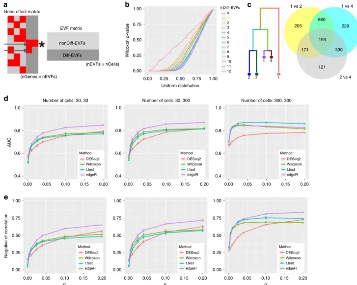
Fig. 6Benchmarking of DE detection methods.aIllustration of how DE genes are generated through the Diff-EVFs. Red squares in the gene effect matrix correspond to non-zero values. The two genes indicated by the arrows are DE genes by number of Diff-EVFs they have (respectively, 2 and 1).bQ–Q plot comparing the p-value obtained from differential expression analysis between subpopulations 2 and 4 (using Wilcoxon test on the true simulated counts) to a uniform distribution. Genes are grouped by the number of EVFs they use and different groups are plotted in different colors. The numbers of Diff-EVFs used by genes can be thought of as the degree of DE-ness. Genes with more Diff-Diff-EVFs have p-values further diverged from uniform distribution.
cVenn diagram showing that closely related populations have less DE genes between them compared to distantly related populations. We use populations 1, 2, 4 as examples: there are much more DE genes from comparison of“1 vs 2”and“1 vs 4”than“2 vs 4”, and DE genes from“1 vs 2”and“1 vs 4”have a big overlap. The DE genes are determined by log2 fold change (LFC) of true counts with criterion |LFC| > 0.8.dThe AUROC (area under receiver operating characteristic curve) of detecting DE genes using four different methods from observed counts with changing capture efficiencyα(σ=0.6). The populations under comparison are 2 and 4. Three sets of criteria were used to define the true DE genes and thefinal performance was the average performance from the three sets: (1)nDiff-EVFgene> 0 and |LFC| > 0.6; (2)nDiff-EVFgene> 0 and |LFC| > 0.8; (3)nDiff-EVFgene> 0 and |LFC| > 1. LFC was calculated with theoretical means from the kinetic parameters.eThe negative of correlation between log2 fold change on theoretical mean of gene-expression and p-values obtained by a DE detection method, with changing capture efficiencyα(σ=0.6). The populations under comparison are 2 and 4. Data used to plotb,d,ecan be found in Source Data
An important distinguishing feature of SymSim is that it provides an intuitive way for generating case studies for DE
analysis that consist of multiple subpopulations with a predefined
structure of similarity. To illustrate this, consider populations 1, 2,
and 4 (Fig.6c), which form a hierarchy (2 and 4 are closer to each
other and similarly distant from 1). This user-defined structure is
reflected in the sizes of the sets of DE genes, obtained,
respectively, from populations 1 vs 2 (1229 genes), 1 vs 4 (1412 genes), and 2 vs 4 (815 genes). Consistent with the hierarchy, the
first two gene sets are overlapping and larger than the third one.
As an example for a benchmark study, we used four methods
to detect DE genes: edgeR45, DESeq246, Wilcoxon rank-sum test,
and t-test on observed counts generated by various parameter
settings (Methods, Supplementary Table 7). We tested the effect
of the total number of cells (N) and mRNA capture rate (α) with
10 simulation runs per parameter configuration. We use two
accuracy measures: (a) AUROC (area under receiver operating characteristic curve), obtained by treating the p-values output
from each method as a predictor (Fig.6d, Methods); (b) negative
of Spearman correlation between the p-values of each detection method and the log fold difference of the true expression levels
(Fig.6e, Methods).
From Fig.6d–e, one can observe that when the numbers of
cells are small (30 in each population), edgeR has the best performance while the other three methods are comparable to each other. When the numbers of cells of both populations
increase to 300, the two naive methods Wilcoxon test and t-test
improve in their relative performance, compared to edgeR and DESeq2. The case where the numbers of cells are 30 and 300 appears to have performance between those of the 30 vs 30 case
and the 300 vs 300 case. When increasing capture efficiency, all
methods gain performance except for the case of AUROC with 300 cells. In that case, the drop in AUROC for some methods is
caused by inflation in p-values asα increases, which results in
lower specificity (Supplementary Fig. 9b). Notably, we noticed
that the adjusted p-values from DESeq2 can have many missing
entries (NAs), especially whenαis low (and thus counts are low),
and therefore we used its unadjusted p-values in Fig. 6d–e.
However, this assignment of NAs in practice filters out genes,
which do not pass a certain threshold of absolute magnitude
(explained in DESeq2 vignette47). To make use of thisfiltering,
we conducted an additional analysis where we used the adjusted p-values for DESeq2 and compare it to all other methods using
only the non-filtered (non NA) genes (Supplementary Fig. 9c). As
expected, the performance of all methods (and specifically
DESeq2) improves when considering only this set of genes, and
converges to high values already at lower capture efficiency rates.
To summarize, we find that edgeR has the best overall
performance, with thet-test rank second followed by Wilcoxon
test. This ranking is consistent with results from a recent paper which evaluated 36 methods for DE analysis with single cell
RNA-Seq data48.
We also investigate the effects of bimodality (controlled by
parameter bimod) on the performance of clustering and
differential expression algorithms. This analysis is presented in
Supplementary Note 6 and Supplementary Figs. 8a–b and 10a–d.
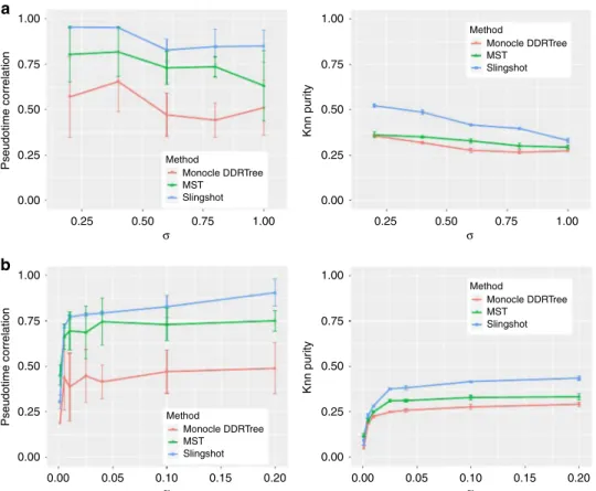
Using SymSim to evaluate trajectory inference methods. The
ability of SymSim to generate a continuum of cell states makes it a convenient choice to benchmark trajectory inference methods.
We compare three methods including Monocle49,50, Slingshot51,
and a minimum spanning tree (MST) algorithm implemented in
the package dynverse52 (Methods). We generate datasets with
different values ofσandαwith the input tree shown in Fig.3a.
For each parameter configuration, we repeat the simulation 10
times. To evaluate the trajectory inference methods, we use two measures: (1) Spearman correlation between true cell order and inferred cell order. We consider cells on each lineage (a path from root to a leaf) separately and take the average of correlation on all
five lineages. (2)k-nearest neighbor purity (knn purity) of cells,
that is, for each cell, we calculate the Jaccard Index between its
k-nearest neighbors in the true trajectory and that in the inferred
trajectory. Results are shown in Fig.7. In these plots,kis set to
100. In Fig.7a, we varyσandfixαas 0.1. Both the correlation and
knn purity decrease whenσincreases. In Fig.7b, we varyαandfix
σas 0.6. All methods show an overall increasing trend along with
α with both measures. Consistent with a recent benchmark
study52, we observe that overall Slingshot clearly outperforms the
other two methods.
Experimental design. Deciding how many cells to sequence is a
decision many researchers face when designing an experiment, and the optimal number of cells to sequence highly depends on the nature of the biological system under investigation and the respective technical hurdles. A previous approach to this
pro-blem53 assumes that the goal of the experiment is to identify
subpopulations of cells and provides a theoretical lower bound for the problem. This bound considers the aspect of counting cells (namely, sequencing enough representative cells from each
sub-population), but it does not account for the identifiability of each
subpopulation, which may be hampered by both technical and biological factors as well as the performance of clustering algorithms.
In the following we demonstrate how SymSim can be used to shed more light on this important problem. Importantly, in its current form SymSim does not use real data to model between-population variability. We therefore interpret the results in a
relative manner—how do different variability factors shift the
required number of cells, compared to each other and to the theoretical lower bound. Our example focuses on a case of one rare subset, represented by cells from population 2 (using the
same tree in Fig. 6c; note that one can easily generalize this
procedure to multiple rare subpopulations). We simulate
observed counts with numbers of cells (N) ranging from 600 to
7000. These simulations were based on the parametersfit to the
cortex dataset38with varying levels ofσandα(250 simulations
per parameter configuration).
We applied the same four clustering methods as described in
the previous section (k-means with scVI or PCA, Louvain
clustering with PCA (Seurat) and SIMLR). We say that a given algorithm was successful in detecting the rare population if at least 50 cells from this set are assigned to the same cluster, and form at least 70% of the cells in that cluster. We use these labels to
compute an empirical success probability P for each algorithm
and each parameter configuration. Out of the 250 simulations for
each parameter configuration, we randomly sample 100
rando-mizations 20 times, and for each 100 randorando-mizations we can
calculate a value of P. We then plot the mean and standard
deviation as error bars of the 20 values ofPfor eachNunder each
configuration (Fig.8a–d, Supplementary Fig. 11). To get an upper
bound on performance that better reflects the data (rather than
the choice of algorithm), we take the bestPout of all algorithms,
and apply cubic spline smoothing (gray curves, Fig. 8a–d). In
each plot we also include the theoretical limit which only requires the presence of at least 50 cells from the rare subpopulation (Methods). The theoretical curve (which is independent of all
parameters exceptN) reaches almost 1 atN=1400. Conversely,
the empirical curves vary dramatically, based on parameter
values. For an easy case of low within-population variability (σ=
bound curve is close to the theoretical one (Fig.8a). This curve decreases when increasing the effect of either nuisance factor
(Fig.8b–c). The reduction is substantially more dramatic for most
of the methods when both nuisance factors increase, while Seurat remains robust to this change, potentially due to that the graph-based clustering method is advantageous in reducing false
positives for the rare population compared to k-means (Fig.8d).
To understand the implications on the number of cells required in a given setting, we calculated how many cells are
required, in each configuration, to achieve a success rate of
respectively 0.6, 0.7, 0.8, and 0.9 (Fig. 8e). As expected, the
resulting numbers can be much higher than the theoretical lower bound. For example, to achieve a success rate of 0.9, when the
within-population variability increases (σ=0.7), we need at least
3838 cells (corresponding toα=0.01), while with the theoretical
curve, we need only less than 1200 cells. In general, the number of
cells needed increase when the desired success rate andσincrease.
Very low capture efficiency (α=0.001,α=0.005) tend to require
high number of cells. Considering only the binomial sampling of cells may therefore underestimate the number of cells needed for a realistic scenario, and considerations of biological and technical variations with simulators like SymSim is merited.
Discussion
SymSim has the following features, which are advantageous over existing simulators: (i) We simulate true transcript counts from a kinetic model that can be interpreted in terms of transcript synthesis rate, promoter activation, and deactivation. (ii) When generating multiple discrete or continuous populations, instead of generating biological differences through directly altering the true transcript count distribution, we set Diff-EVFs, which can be interpreted as biological conditions that cause the differences
between subpopulations of cells. This is a more natural and realistic way to simulate biological transcriptional differences. (iii) The EVF formulation provides an intuitive way to specify and
simulate complex structures of cell–cell similarity, without the
need for manual specifications of the numbers of DE genes13. (iv)
When generating observed counts, we simulate key steps in real experimental protocols, which automatically gives us dropout events, length bias, and distribution of library sizes. We also provide choices to use UMI-based protocols or non-UMI full-length mRNA protocols, as the properties of data output from these two categories can be very different.
The main input parameters to SymSim, mostly the parameters in the third knob, are self-explanatory with their own technical meanings, which users can adjust to match an experimental dataset of interest. SymSim allows users to simulate datasets with desired properties or matched with experimental data. While the
procedure of parameterfitting was developed in order to generate
simulated datasets with similar properties, it may also provide additional insight, as the parameters are biologically or
techni-cally interpretable. For instance, comparing the parametersfit to
the the UMI and non-UMI datasets in this study we note that the
capture efficiency inferred to the latter is much higher
(Supple-mentary Tables 2–5). The modular nature of SymSim provides
possibilities to generalize its application. For example, the gen-eration of true counts with EVFs and transcription kinetics can be replaced by learning a generative model from real data, with
methods such as scVI4. This type of extension will facilitate
simulation of between-subpopulation diversity that better mimics experimental observations, albeit at the cost of using parameters that are less interpretable biologically. Another extended appli-cation of interest is to use different tree structures for different Diff-EVFs when generating multiple populations of cells, such
1.00 a b 0.75 Pseudotime correlation Pseudotime correlation Knn pur ity Knn pur ity 0.50 0.25 0.00 1.00 0.75 0.50 0.25 0.00 1.00 0.75 0.50 0.25 0.00 0.25 0.00 0.05 0.10 α 0.15 0.20 0.00 0.05 0.10α 0.15 0.20 0.50 σ 0.75 σ Method Monocle DDRTree MST Slingshot Method Monocle DDRTree MST Slingshot Method Monocle DDRTree MST Slingshot Method Monocle DDRTree MST Slingshot 1.00 1.00 0.75 0.50 0.25 0.00 0.25 0.50 0.75 1.00
Fig. 7Benchmark trajectory inference methods.aPseudotime correlation and knn purity of all methods when varyingσ(α=0.1).bPseudotime correlation and knn purity of all methods when varyingα(σ=0.6). Data used to plota,bcan be found in Source Data
that every tree represents a different aspect of variability between cells. For instance, using this approach, one tree can represent a differentiation process and the other can represent variability due to the physical location of the cell.
As the number and extent of biological applications of single cell genomics continues to grow, so does the extent of analytical questions one can tackle, which go beyond standard bulk era
analysis steps (e.g., trajectory analysis, mRNA velocity54, and
more). The need for robust analytical methods therefore increa-ses, and so does the means for proper evaluation of these methods. SymSim provides a starting point to address this
chal-lenge of flexible and feature-rich simulation for method
evalua-tion, as it aims to directly mimic the key mechanistic properties of single cell RNA sequencing.
Methods
Simulating gene expression with the kinetic model. As shown in Fig.2a, the kinetic model of gene expression considers that a gene can be eitheronoroffand the probabilities to transit between the two states arekonandkoff. When the gene is
onit is transcribed with transcription rates. The transcripts degrade with rated. For a given gene, based on these parameters one can simulate the number of its transcript molecules over time. The theoretical probability distribution can be calculated via the Master Equation15,17, which is the steady state solution for the
kinetic model. Alternatively, the kinetic model can be represented by a Beta-Poisson model17, which we use in our implementation to sample expression values
for a gene.
Calculating parameters for the kinetic model in SymSim. For a gene in a cell, the parameters for the kinetic modelkon,koff, andsare calculated from the
cell-specific EVF vectors of this cell and the gene effect vectors of the gene (Fig.2a). To allow independent control of the three parameters, we use one EVF vector and one
a e σ = 0.65, α = 0.1 σ = 0.4, α = 0.005 σ = 0.65, α = 0.005 σ = 0.4, α = 0.1 b c d α σ Prob(success) = 0.6 Prob(success) = 0.7 1000 3000 5000 7000 0.0 0.2 0.4 0.6 0.8 1.0 Number of cells 1000 3000 5000 7000 Number of cells 1000 3000 5000 7000 Number of cells 1000 3000 5000 7000 0.40 0.001 0.005 0.010 0.025 0.040 0.100 0.001 0.005 0.010 0.025 0.040 0.100 0.001 0.005 0.010 0.025 0.040 0.100 0.001 0.005 0.010 0.025 0.040 0.100 0.60 0.65 0.70 0.80 0.40 0.60 0.65 0.70 0.80 0.40 0.60 0.65 0.70 0.80 0.40 > 7000 7000 6000 5000 4000 3000 2000 0.60 0.65 0.70 0.80 Number of cells Probability 0.0 0.2 0.4 0.6 0.8 1.0 Probability 0.0 0.2 0.4 0.6 0.8 1.0 Probability 0.0 0.2 0.4 0.6 0.8 1.0 Probability PCA+kmeans SIMLR scVI+kmeans PCA+Louvain (Seurat) Theo Fitted max PCA+kmeans SIMLR scVI+kmeans PCA+Louvain (Seurat) Theo Fitted max PCA+kmeans SIMLR scVI+kmeans PCA+Louvain (Seurat) Theo Fitted max PCA+kmeans SIMLR scVI+kmeans PCA+Louvain (Seurat) Theo Fitted max Prob(success) = 0.8 Prob(success) = 0.9
Fig. 8The number of cells needed to detect a rare population. We generatefive populations according to the tree structure shown in Fig.3and set population 2 as the rare population which accounts for 5% of the cells. Other populations share 95% of the cells evenly. The criteria of detecting the rare population are that at least 50 cells from this population are correctly detected and the precision (positive predicted value) is at least 70%.a–dThe probability of detecting the rare population when sequencingN(x-axis) cells under differentσandαconfigurations, with different clustering methods. The black curve represents the theoretical probability from the binomial model, assuming that all cells sequenced are assigned correctly to the original population. The gray curve with transparency takes the maximum value at each data point from all four clustering methods with smoothing. Error bars are standard deviation over 20 randomizations.eThe heatmaps show the number of cells needed to sequence under different configurations ofσandαto detect the rare population with success rates 0.6, 0.7, 0.8, 0.9, always using the best clustering method. Data used to plota–ecan be found in Source Data