Institute of Parallel and Distributed Systems University of Stuttgart Universitätsstraße 38 D–70569 Stuttgart Studienarbeit Nr. 2325
Autonomous docking of
heterogenous robots
Patrick AlschbachCourse of Study: Informatik
Examiner: Prof. Dr. rer. nat. habil. Paul Levi Supervisor: Dipl. Inf. Florian Schlachter
Commenced: 22.12.2010
Acknowledgements
First and for most, I would like to thank the examiner Prof. Dr. rer. nat. habil. Paul Levi at the University of Stuttgart for giving me the chance to be involved in this project.
I would like to thank my supervisor Dipl. Inf. Florian Schlachter. I appreciate the freedom that Florian gave me in choosing the research direction and methods. Along the way I have benefited a lot from the discussion with him.
I am also grateful to Christopher Schwarzer from University of Tübingen for the useful and helpful discussion in hardware programming and programming in C / C++. I would like also to thank Sergej Popesku, Benjamin Girault and all the other colleagues in the lab for all the suggestions and kindness help.
Abstract
This student research project is part of the SYMBRION and REPLICATOR projects. Symbrion and Replicator stands for two different, partly overlapping projects named SYMBRION [Sym10] and REPLICATOR [Rep10], respectively. These two research projects are supported by the European Commission. Their focus is to investigate and develop novel principles of adaptation and evolution for symbiotic multi-robot organisms. These robot organisms consist of super-large-scale swarms of robots. The special feature in the SYMBRION and REPLICATOR projects is that the robots are able to connect to each other. The robot hardware consists of different sensors and actuators. These preconditions enables the dynamically self-organized aggre-gated organisms to solve different tasks. For the development of novel principles bio-inspired and evolutionary algorithms are used.
The focus of this work relies on the development of a mechanism for close co-operation between three different types of robots evolved in the SYMBRION and REPLICATOR projects. These three systems differ in their mode of locomotion and their sensors, as described later. The different robots can move completely free in the area in single mode. At any time, a single robot autonomously decides to form an organism with other robots. To form an organism the single robot has to con-nect firmly with another one. For this reason, the various robots are equipped with docking elements. The aim of this study is an algorithmic solution linking these docking elements.
Contents
List of Figures IX
List of Tables XI
List of Symbols XII
1 Introduction 15
2 Background and Related Work 16
2.1 Swarm Intelligence . . . 16
2.2 Swarm Robotics . . . 18
2.3 Swarm Robots Hardware from Symbrion and Replicator . . . 19
2.3.1 Robot from the University of Karlsruhe . . . 19
2.3.2 Active wheel from the University of Stuttgart . . . 20
2.3.3 Scout robot from SSSA . . . 20
2.4 Behaviour of the robots . . . 21
2.4.1 Flocking . . . 21 2.4.2 Locate Beacon . . . 21 2.4.3 Orientation . . . 22 2.4.4 Alignment . . . 23 2.4.5 Connect . . . 23 2.4.6 In Organism . . . 23 2.4.7 Disconnect . . . 25
2.5 The Docking Element . . . 25
2.6 Dispersion of the infrared diode . . . 25
2.6.1 Robot from University of Karlsruhe . . . 26
2.6.2 Active Wheel from University of Stuttgart . . . 26
2.6.3 Robot from SSSA . . . 27
3 Algorithm for Direct Docking Mechanism 33 3.1 The Inspiration . . . 33
3.2 Algorithmic Solution . . . 34
3.2.1 State Machine . . . 34
3.2.2 Flocking . . . 38
3.2.6 In Organism . . . 53
3.2.7 Disconnect . . . 53
3.3 Experimental Set-Up . . . 55
3.3.1 Experiment 1.1: Active Wheel - Active Wheel . . . 55
3.3.2 Experiment 1.2: Active Wheel - Robot from Karlsruhe . . . 55
3.3.3 Experiment 1.3: Active Wheel - Robot from SSSA . . . 55
3.3.4 Experiment 1.4: Robot from Karlsruhe - Active Wheel . . . 56
3.3.5 Experiment 1.5: Robot from Karlsruhe - Robot from Karlsruhe 56 3.3.6 Experiment 1.6: Robot from Karlsruhe - Robot from SSSA . . 56
3.3.7 Experiment 1.7: Robot from SSSA - Active Wheel . . . 57
3.3.8 Experiment 1.8: Robot from SSSA - Robot from Karlsruhe . . 57
3.3.9 Experiment 1.9: Robot from SSSA - Robot from SSSA . . . 57
3.4 Experiments and Results . . . 58
3.4.1 Result 1.1: Active Wheel - Active Wheel . . . 58
3.4.2 Result 1.2: Active Wheel - Robot from Karlsruhe . . . 58
3.4.3 Result 1.3: Active Wheel - Robot from SSSA . . . 59
3.4.4 Result 1.4: Robot from Karlsruhe - Active Wheel . . . 59
3.4.5 Result 1.5: Robot from Karlsruhe - Robot from Karlsruhe . . . 60
3.4.6 Result 1.6: Robot from Karlsruhe - Robot from SSSA . . . 61
3.4.7 Result 1.7: Robot from SSSA - Active Wheel . . . 61
3.4.8 Result 1.8: Robot from SSSA - Robot from Karlsruhe . . . 62
3.4.9 Result 1.9: Robot from SSSA - Robot from SSSA . . . 62
3.5 Summary and Conclusion of Experiments . . . 63
4 Adjusted Algorithm for Direct Docking Mechanism 70 4.1 The Extension . . . 70
4.2 Algorithmic Solution . . . 71
4.2.1 Orientation . . . 71
4.3 Experimental Set-Up . . . 78
4.3.1 Experiment 2.1: Rotation and docking of the Active Wheel from University of Stuttgart . . . 78
4.3.2 Experiment 2.2: Rotation of the Active Wheel and docking of the robot from Karlsruhe . . . 78
4.3.3 Experiment 2.3: Rotation and docking of the robot from Karl-sruhe . . . 79
4.3.4 Experiment 2.4: Rotation of the robot from SSSA . . . 79
4.4 Experiments and Results . . . 81
4.4.1 Result 2.1: Rotation of the Active Wheel from University of Stuttgart . . . 81
Contents
4.4.2 Result 2.2: Rotation of the Active Wheel and docking of the robot from Karlsruhe . . . 81 4.4.3 Result 2.3: Rotation and docking of the robot from Karlsruhe 82 4.4.4 Result 2.4: Rotation and docking of the robot from SSSA . . . 82 4.5 Summary and Conclusion of Experiments . . . 83
5 Advanced Scenario 88 5.1 Assembling an organism . . . 88 5.2 Rescue scenario . . . 88 6 Conclusion 91 6.1 Summary of Contributions . . . 91 6.2 Future Work . . . 92 Bibliography A
2.1 Green tree ants form a bridge . . . 16
2.2 Collective selection of one foraging path over a diamond-shaped bridge leading to a food source by workers of the Lasius niger ants. . 18
2.3 An overview of the three robots from the different Universities. . . . 20
2.4 A picture of a multi-robot organism - Hexapod . . . 21
2.5 Active Wheel from University of Stuttgart at work. . . 22
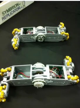
2.6 The Scout robot from SSSA. . . 23
2.7 State machine - Behaviour . . . 24
2.8 Expanded docking mechanism. . . 26
2.9 The active docking element of the robot from SSSA. . . 27
2.10 The passive docking element of the Active Wheel. . . 27
2.11 After docking - The active element is closed. . . 28
2.12 The active docking element of the robot from Karlsruhe. . . 28
2.13 Schematic of sensor position. . . 29
2.14 Infrared data of the robot from University of Karlsruhe. . . 30
2.15 Infrared data of the Active Wheel from Stuttgart. . . 31
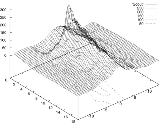
2.16 Infrared data of the Scout from University of SSSA. . . 32
3.1 Locate Beacon - Simple Situation . . . 33
3.2 Experimental set-up with two Active Wheels. . . 55
3.3 Experimental set-up with Active Wheel and the robot from Karlsruhe. 56 3.4 Experimental set-up with Active Wheel and the robot from SSSA. . . 57
3.5 Experimental set-up with robot from Karlsruhe and the Active Wheel. 58 3.6 Experimental set-up with two robots from Karlsruhe. . . 59
3.7 Experimental set-up with robot from Karlsruhe and the robot from SSSA. . . 60
3.8 Experimental set-up with robot from SSSA and the Active Wheel. . . 61
3.9 Experimental set-up with robot from SSSA and the robot from Karl-sruhe. . . 62
3.10 Experimental set-up with two robots from SSSA. . . 63
3.11 Robot from Karlsruhe is docking with Active Wheel. . . 64
3.12 Robot from SSSA is docking with Active Wheel. . . 65
3.13 Active Wheel is docking with Robot from Karlsruhe. . . 66
List of Figures
3.15 Active Wheel is docking with Robot from SSSA. . . 68
3.16 Robot from Karlsruhe is docking with Robot from SSSA. . . 69
4.1 Locate Beacon - Complicated Situation . . . 70
4.2 Orientation logic - At the beginning . . . 75
4.3 Orientation logic - After one rotation . . . 76
4.4 Orientation logic - After second rotation . . . 77
4.5 Experimental set-up with Active Wheel and the robot from SSSA . . 78
4.6 Experimental set-up with Active Wheel and the robot from Karlsruhe 79 4.7 Experimental set-up with the robot from Karlsruhe and the Active Wheel . . . 80
4.8 Experimental set-up with the Active Wheel and the robot from SSSA 81 4.9 Active Wheel rotates before it is docking with robot from SSSA. . . . 84
4.10 Active Wheel rotates before the robot from Karlsruhe docks to it. . . 85
4.11 The robot from Karlsruhe rotates before it is docking with the Active Wheel. . . 86
4.12 Robot from SSSA rotates until it finds the beacon for docking. . . 87
5.1 The three Symbrion and Replicator robots assemble an organsim. . . 89 5.2 The three Symbrion and Replicator robots perform a rescue scenario. 90
sruhe . . . 42 3.2 Possible assignment of the transmitted beams of the Scout robot from
SSSA . . . 43 3.3 Possible assignment of the transmitted beams of the Active Wheel . . 44
List of Abbreviations
AS Alignment Signal: Robots are aligned
CPB Connection Possible Beacon: A beacon with the information “Con-nection Possible”
DS Disconnection Signal: Robots are successfully disconnected ICR In Connection Range: In the range to connect / close docking
element
NCPB No Connection Possible Beacon: A beacon with the information “No Connection Possible”
NS No Signals: Signal lost
OM Organism Mode: Signal for the robot to organize into an organ-ism
SSSA Scuola Superiore Sant’Anna - Italy
1 Introduction
This student research project has set a target to deal with the docking of three different robots of the SYMBRION and REPLICATOR projects. SYMBRION and REPLICATOR represent two large-scale integrated research projects , supported by the European Commission, dealing with a new research initiative in the domain of swarm robotics. SYMBRION is strongly focused on evolve-ability of organisms and is exploring artificial evolution in robotic population. REPLICATOR focuses on more application-related aspects, e.g. reconfigurability of sensors and actuation, with the main goal of creating mobile and adaptable sensor networks for indoor environments. The main idea of these projects originates from a biological obser-vation of symbiotic organisms. In our case an individual robot is able to dock to an other one and build complex multi-cellular organisms, like cells can do. To do this, the various robots are equipped with a special docking element. After the docking process the organisms have additional functionality and can solve different tasks. Individual robots can also be used as an energy source for the whole organism. When the need of aggregation is over, these organisms can disaggregate and exist further as stand-alone cells. In this student research project the mechanisms for docking is explored and represented.
This work starts with an overview of swarm intelligence (Chapter 2.1) and swarm robotics (Chapter 2.2). After the introduction three different robot types are intro-duced (Chapter 2.3) and the behaviour of the robots is described (Chapter 2.4). For the later algorithm, the relevant parts, such as the docking element (Chapter 2.5) and the infrared diode (Chapter 2.6) are described in great detail in an own section. As part of the work the native docking approach is presented in Chapter 3. The idea and the algorithmic solution itself will be shown in Chapter 3.1 respectively in Chapter 3.2. Chapter 3.3 deals with different experiments. Their results are rep-resented in the following Chapter 3.4. As expected in the native approach, which is that the robots are faced to each other, the algorithm will be extended. In the following Chapter 4, an extended solution is presented, in which the robot rotates before the connection. Also the idea (Chapter 4.1) and the implementation (Chap-ter 4.2) is shown in this work. This has also been tested (Chap(Chap-ter 4.3) by various experiments and the results are shown in Chapter 4.4. In Chapter 5 one can find two different contributions of the developed algorithm. Chapter 6 summarizes and discusses this student research.
The term “swarm intelligence” was first introduced by Beni and Wang (1989) [BW89]. They used this term to describe their work on cellular robots. The definition of swarm intelligence has been expanded again in 1999 by Bonabeau et al. [BDT99] Bonabeau et al. used the new definition to describe algorithms which are designed for collective behaviour of social insect colonies. He was inspired by resurrected animal societies. Swarm intelligence is deeply embedded in the biological study of self-organised behaviours of social insects. Natural examples of swarm intelligence
Figure 2.1: Green tree ants form a bridge. [oT11]
systems include colonies of ants and termites, schools of fish or even crowds of hu-man beings. In a swarm intelligence system, a large population of simple agents interact locally with each other and with the environment.
The background of swarm behaviour is that simple behaviour of agents produce complex collective behaviour. This is done without centralized control, arising from interactions. There are several hidden mechanisms, such as self-organization, behind the organization without an organizer. Self-organization relies on four main
2.1 Swarm Intelligence
parts:
• positive feedback • negative feedback
• balance of exploitation and exploration • multiple interactions
The interplay of positive and negative feedback leads to different phenomenas. The positive feedback typically promotes the creation of structures and amplifies the fluctuations of the system. Conversely, negative feedback serves as a regulatory mechanism to counterbalance positive feedback and helps to stabilize the collective pattern.
Dorigo and Birattari (2007) proposed an alternative definition:
“Swarm intelligence is the discipline that deals with natural and artifi-cial systems composed of many individuals that coordinate using de-centralized control and self-organisation. In particular, the discipline focuses on the collective behaviours that result from the local interac-tions of the individuals with each other and with their environment.” [DB07]
In addition, they pointed to the following things: The swarms consist of a greater number of individuals. These individuals are relatively homogeneous. Interaction between individuals is based on simple rules of behaviour which only use local information. That information is sent directly. Alternatively, an information ex-change using Stigmergy (local information that the individuals exex-change directly or via the environment) is possible. The overall behaviour of the group results from the conduct of the individual or by the interaction of the individual with the envi-ronment.
A fine example of swarm intelligence in nature is the behaviour of ants. By us-ing pheromones ants are able to solve the travelus-ing salesman problem, findus-ing an optimal path between food source and their home colony. See Figure 2.2.
Figure 2.2: Collective selection of one foraging path over a diamond-shaped bridge leading to a food source by workers of the Lasius niger ants. [BDT99]
2.2 Swarm Robotics
In the field of robotics there are many different names for a larger group of robots, such as cellular robotics (Beni, 1988) [Ben88] , collective robotics (Kube and Zhang, 1993) [KZ93] and large-scale micro robots (Dudenhoeffer and Jones, 2000) [DJ00]. Regarding a biological background the concept of the swarm is introduced later. Since the term “swarm” is used in many scientific fields, there was a mixtures of terminology.
¸Sahin proposed 2005 the following definition:
“Swarm robotics is the study of how a large number of relatively simple physically embodied agents can be designed such that a desired collec-tive behaviour emerges from the local interactions among the agents and between the agents and the environment”[SS05]
In addition, some criteria have been defined, as mentioned previously in Chapter swarm intelligence. In the field of robotics a swarm is defined as a larger number of robots which promotes scalability. Each robot in the swarm has only limited coverage, communication and calculation skills. That leads to the situation, that in general a task can not be performed by a single robot because of its relative incapacity or inability.
2.3 Swarm Robots Hardware from Symbrion and Replicator
2.3 Swarm Robots Hardware from Symbrion and Replicator
This essay is part of the SYMBRION and REPLICATOR projects. These two projects have different research focuses:SYMBRION, SYMBRION Enlarged EU
• platform for exploring artificial evolution and pervasive evolve-ability • extremely powerful computational on-board resources
• support for artificial immunology and embryology • large number of light modules
• powerful on-boad and off-board simulator
REPLICATOR
• intelligent, reconfigurable and adaptable “carrier” of sensors (sensors net-work)
• sensors- and communication-rich platform • high-reliable in open-end environment • medium number of heavy modules
In terms of research projects, three different robotic platforms (Figure 2.3) have been developed which are presented below.
2.3.1 Robot from the University of Karlsruhe
The robot from University of Karlsruhe is designed as a very stable cube with dif-ferent sensors and actuators. It can be used as a single robot and as well as a stable backbone of an multi-robot organism. The robot is able to move on the ground with the aid of two screws. The main elements of the robot is the hinge in the middle, and the four connectors on all of its four sides. This elements enable the robots to form an organism, like a hexapod, which is shown below in Figure 2.4.
Figure 2.3: An overview of the three robots. From left to right, the robot from the University of Karlsruhe, the Active Wheel from University of Stuttgart and the Scout robot from Scuola Superiore Sant’Anna -Italy (SSSA). [LK10]
2.3.2 Active wheel from the University of Stuttgart
The Active Wheel evolved by a research team of the University of Stuttgart is a special tool module, that is able to expand the functionality of other robots. Like the “backbone” robot from University of Karslruhe, the Active Wheel can act by itself or form organisms. For example, the Active Wheel has the possibility to raise and move other robots or organisms or act as an extra energy source for robots involved in the organism built. Furthermore, the Active Wheel can be used to rescue fallen robots (Figure 2.5).
2.3.3 Scout robot from SSSA
The Scout robot from SSSA - Scuola Superiore Sant’Anna (Italy) is a different type of robot. This robot is able to organize in organisms like the other two robots as well. In addition, it is specialized in fast and flexible locomotion that can be used for inspection of the environment. For example, the robot can be attached at the periphery of an organism to explore the environment (Figure 2.6).
2.4 Behaviour of the robots
Figure 2.4: A picture of a multi-robot organism. The 24 single robots are connected to one big organism called hexapod. [Sym10]
2.4 Behaviour of the robots
The behaviour of the robots describes a state machine (Figure 2.7) filled with differ-ent controllers. This chapter contains the description of the differdiffer-ent states, or the behaviour of each robot within the state machine.
2.4.1 Flocking
In the initial state the robots are moving randomly in the arena and avoid obsta-cles. They constantly read the values of the sensors in the direction of travel. If an obstacle is detected within a critical distance, a robot tries to avoid it. The easiest way is simple turning, until an obstacle is detected. When a robot receives a signal that it should build an organism, the state machine switches to the state “Locate Beacon”. This organism signal (Organism Mode Signal - OM ) can be sent from various sources e.g. remote control, neural network etc. An independent decision to form an organism would be the ideal approach. The origin of this signal is not part of this work. It is simply assumed to be preceded by default.
2.4.2 Locate Beacon
When a robot was commanded to organize himself into a body, it first tries to find a binding partner. The robots have the ability to emit infrared signals from remote units. Therefore the robot is sending from the side, on which it wants to connect with another robot, a specific beacon signal (Connection Possible Beacon - CPB). On the remaining other faces a different signal is transmitted (No Connection Pos-sible Beacon - NCPB). Refer to the tables 3.1, 3.2 and 3.3. The robots move
ran-Figure 2.5: This is a scenario in which two Active Wheels carry a defective element. [LK10]
domly through the area while looking for a CPB. Once a robot has found a CPB, it’s state machine enters the state “Alignment” (Figure 2.7). An approached and improved version of the robot’s controller responds to NCPB signals as well. Such a signal switches the robot’s current state into “Orientation”. The “Orientation” state extends the state machine in the way that a robot first adapts its orientation accordingly before aligning to another possible docking partner.
2.4.3 Orientation
If a NCPB signal is received, a robot has found a partner to connect to. At this point usually the robots are not aligned properly yet for the binding. For adjust-ing the appropriate position between the two connection partners there are two approaches as follows:
• one robot moves, while the other robot remains stationary
• both robots adapt that positions simultaneously towards each other
In this work the first approach is used and described subsequently. The easiest way of adjusting a robot’s position is by rotation. Therefore, one robot rotates around as long as the transmission side and the receiver side of the CPB signal doesn’t correspond. As soon as the moving robot reached the correct position, it stops. The robots now face each other with their docking elements and the state machine enters the “Alignment” state. If the signal gets lost during the alignment procedure the state machine changes back to the “Locate Beacon” state and restarts to locate a binding partner.
2.4 Behaviour of the robots
Figure 2.6: Connected Scout robot that explores its environment. [LK10]
2.4.4 Alignment
The “Alignment” state defines the robots to face their docking elements, they are going to connect appropriate. In this state the robots try to minimize the gap be-tween their docking elements and to optimally align their position so they just have to move straight forward in one direction for the docking. An optimal alignment can be achieved during the alignment procedure by using the Braitenberg-Vehicle-Algorithm. The docking robot will follow the maximum of the CPB signal until it reaches a critical distance to the other robot. When reaching this critical distance the state machine switches to the “Connect” state. If the signal gets lost, the state machine changes back to the “Locate Beacon” state.
2.4.5 Connect
The “Connect” state takes care of the last step of joining. The elements get docked now and the active docking elements get closed. After that the state machine enters the “In Organism” state. If the signal gets lost, the state machine changes back to the “Locate Beacon” state.
2.4.6 In Organism
After a successfully connection the two robots build an organism and do not act in-dividually anymore. Each step forward is executed cooperatively. Remaining free docking elements continue linking to other available connection partners until the signal to disconnect is received. The signal to leave this state (no more Organism Mode Signal - !OM) can be send from various sources e.g. remote control, neural
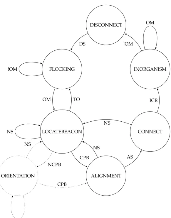
FLOCKING LOCATEBEACON ALIGNMENT ORIENTATION CONNECT INORGANISM DISCONNECT !OM OM TO CPB NS NS AS NS ICR OM !OM DS NCPB CPB NCPB NS
Figure 2.7: State machine - This state machine shows the behaviour of the robot. Start state is the “Flocking” state. The transitions have been marked with abbreviations. They can be looked up in the abbreviation table at the beginning of the document. The exclamation mark corresponds to the negation of the statement.
2.5 The Docking Element
network etc. An ideal approach to separate an organism would be a self-organized decision. The origin of this signal is not part of this work.
2.4.7 Disconnect
This state handles the separation of previously connected robots. By disconnecting the interconnection between two robots their docking elements open and one of the robots will move away. The state machine returns to the “Flocking” state. By doing so, each robot changes back its mode to separated.
2.5 The Docking Element
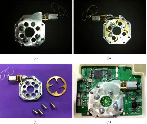
A relevant part of the docking mechanism is the docking element. For this reason, this section will describe this component briefly. There are active and passive dock-ing elements installed in the robots. In Figure 2.8 can be seen the expanded active docking element from the front (a) and rear (b). In the picture (c) is the component completely broken down into its component parts. Where image (d) shows the built-in docking element. It can be seen that the active docking element contains a drive. This drive runs a screw which is used to close or open the docking element. The opening and closing is performed by a shift of a metal disk, which can be seen in the image (c) on the right. In addition, all docking element are unisexual. Thus, each element can dock to each other. In Figure 2.9 an active docking element from the robot from SSSA is shown. In Figure 2.10 a passive docking element from Ac-tive Wheel from University of Stuttgart can be seen. This docking element alone can not form a connection. It must get connected to an active element for a solid connection. In Figure 2.11 two robots have a solid connection with closed docking elements.
2.6 Dispersion of the infrared diode
For the implementation of the later algorithm the infrared diode plays an important role. Therefore, this component is described briefly. It reviews the position of the transmitter and receiver. To demonstrate the correctness of the algorithm a drawing of the measurements for each robot is added. Because it can not be assumed that the radiation pattern is correct and there is only one intensity maximum. Normally, the transmitted beam containing only one intensity maximum in the middle. If this were not the case, the algorithm would not work. In Figure 2.12 we see again the docking element. In Figure 2.13 is shown a schematic. Above the docking element is the diode that was used to send the beam (LED0). Left (IR6) and right (IR7) are the two receivers.
(a) (b)
(c) (d)
Figure 2.8: Expanded docking mechanism.
2.6.1 Robot from University of Karlsruhe
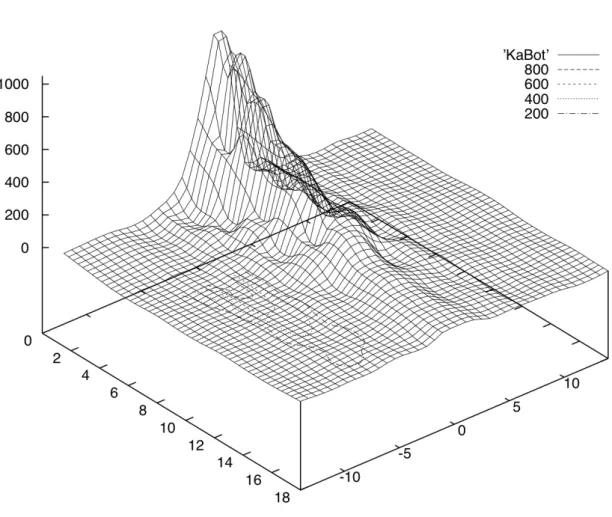
The picture 2.14 shows the measurements of one infrared sensor of the Active Wheel. A infrared beam was sent from the infrared diode in the middle of the top of the robot from University of Karlsruhe. As can be seen in picture the sensor value distribution has an unique maximum in the middle. This shows that the in-frared beam can be used to find the middle of the docking element. It must always go in the direction of the gradient to reach the maximum. This procedure is used later in the implementation.
2.6.2 Active Wheel from University of Stuttgart
The picture 2.15 shows the measurements of one infrared sensor of the robot from University of Karlsruhe. A infrared beam was sent from the infrared diode in the
2.6 Dispersion of the infrared diode
Figure 2.9: The active docking element of the robot from SSSA.
Figure 2.10: The passive docking element of the Active Wheel.
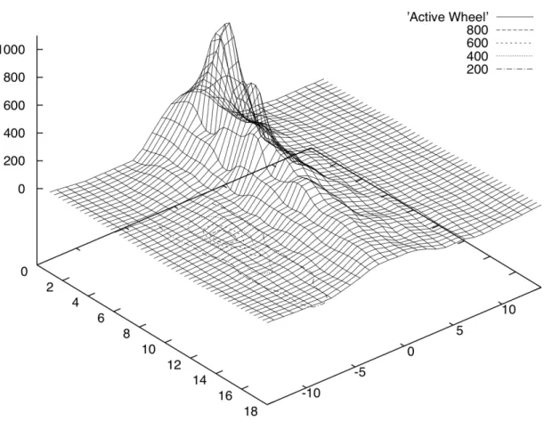
middle of the top of the Active Wheel from University of Stuttgart. As can be seen in picture the sensor value distribution has an unique maximum in the middle. This shows that the infrared beam can be used to find the middle of the docking element. The robot must always go in the direction of the gradient to reach the maximum. This procedure is used later in the implementation.
2.6.3 Robot from SSSA
The picture 2.16 shows the measurements of one infrared sensor of the Active Wheel. A infrared beam was sent from the infrared diode in the middle of the top of the Scout robot from University of SSSA. As can be seen in picture the sensor value distribution has an unique maximum in the middle. This shows that the in-frared beam can be used to find the middle of the docking element. The robot must always go in the direction of the gradient to reach the maximum. This procedure is used later in the implementation.
Figure 2.11: After docking - The active element is closed.
2.6 Dispersion of the infrared diode
2.6 Dispersion of the infrared diode
3 Algorithm for Direct Docking
Mechanism
3.1 The Inspiration
A part of this paper is dedicated to search for an algorithmic solution to the dock-ing maneuver. The first approach assumes the robots facdock-ing their fronts they want to connect, as shown in Figure 3.1. In this example robot A remains stationary while robot B moves randomly in the arena (random walk with collision avoid-ance). When A decides to get connected it sends a connection possible beacon (CPB). With the help of an external signal, robot B begins to search for the CPB. Receiving a CPB signal, it aligns itself and begins to move towards robot A. Once the docking elements have been hooked up the connector is closed.
A B
Figure 3.1: Locate Beacon - Simple Situation: Each robot has an active face that is ready for docking (CPB Signal). The three remaining sides stay inactive and are not ready for docking (NCPB Signal). In the simplest case, two robots are facing their active sides. In this case, the state machine enters the “Alignment” state.
This section presents the various algorithmic solutions. 3.2.1 State Machine #include "IRobot.h" #include <assert.h> #include <pthread.h> #include <stdlib.h> #include <signal.h> #include "Common.h" #include <string.h> #include <iostream> using namespace std;
typedef void (* function_t)(void);
typedef enum {
FLOCKING, LOCATEBEACON, ALIGNMENT, ORIENTATION, CONNECT, INORGANISM, DISCONNECT
} state_t; state_t state;
RobotBase::RobotType robotType; IRValues ir_values;
bool bOrganismMode = false; //external signal default: false bool bNoConnectionPossibleBeacon = false; //default: false bool bConnectionPossibleBeacon = false; //default: false bool bAligned = false; //default: false
bool bConnected = false; //default: false bool bDisconnected = false; //default: false
pthread_t input_thread; pthread_mutex_t cin_read;
void* input_thread_fct(void* p) {
while(true) { cin.get(); bOrganismMode = !bOrganismMode; } return NULL; }
3.2 Algorithmic Solution
inline void startCinRead(void) { pthread_mutex_init(&cin_read,NULL);
pthread_create(&input_thread, NULL, input_thread_fct, NULL); usleep(10000);
}
// handle states
void handleFlocking(int approaching_side) { flockingRandomWalk(approaching_side); cout << "Flocking" << endl;
if (bOrganismMode) { state = LOCATEBEACON; } else { state = FLOCKING; } }
void handleLocateBeacon(int approaching_side) { locateBeaconBraitenberg(approaching_side); cout << "LOCATE BEACON" << endl;
if (bConnectionPossibleBeacon) {
//beacon found
state = ALIGNMENT;
} else if (bNoConnectionPossibleBeacon){
//no beacon found
state = ORIENTATION; } else if (!bOrganismMode){
//no beacon found
state = FLOCKING; } else {
//no beacon found and timeout
state=LOCATEBEACON; }
}
void handleOrientation(int approaching_side) { cout << "ORIENTATION" << endl;
if (true) {
state = ALIGNMENT; } else if (false) {
} }
void handleAlignment(int approaching_side) { alignment(approaching_side);
cout << "ALIGNMENT" << endl;
if (bAligned) { state = CONNECT; } else { state = LOCATEBEACON; } }
void handleConnect(int approaching_side) { cout << "CONNECTION" << endl;
connect(approaching_side); if (bConnected) { state = INORGANISM; } else if (bConnectionPossibleBeacon) { state = CONNECT; } else { state = LOCATEBEACON; } }
void handleInOrgansim(int approaching_side) { cout << "ORGANISM" << endl;
if (bOrganismMode) { state = DISCONNECT; } else { state = INORGANISM; } }
void handleDisconnect(int approaching_side) { disconnect(approaching_side);
if (!bDisconnected) { state = DISCONNECT;
3.2 Algorithmic Solution
} else {
state = FLOCKING; }
}
// return 0 if OK, 1 exit, < 0 error int state_machine(int approaching_side) {
switch (state) { case FLOCKING: handleFlocking(approaching_side); break; case LOCATEBEACON: handleLocateBeacon(approaching_side); break; case ALIGNMENT: handleAlignment(approaching_side); break; case ORIENTATION: handleOrientation(approaching_side); case CONNECT: handleConnect(approaching_side); break; case INORGANISM: return 1; handleInOrgansim(approaching_side); break; case DISCONNECT: handleDisconnect(approaching_side); break; default: assert(0); break; } usleep(1000); return 0; }
void interrupt_signal_handler(int signal) {
if (signal == SIGINT) { RobotBase::MSPReset(); exit(0);
} }
int main(int argc, char** args) {
SPIVerbose = ERROR;
robotType = RobotBase::Initialize();
// set SIGTERM handler (MSP reset before quitting) struct sigaction a;
a.sa_handler = &interrupt_signal_handler; sigaction(SIGINT, &a, NULL);
// set initialstate state = FLOCKING; int approaching_side = 0; if (argc > 1) { approaching_side = atoi(args[1]); } startCinRead(); while (bContinue) { switch (state_machine(approaching_side)) { case 0: break; case 1: bContinue = false; break; default: assert(0); break; } } } Algorithms 3.1: main.cpp
This code shows the implementation of the state machine shown in Figure 2.7. 3.2.2 Flocking
In Flocking mode, robots move randomly through the arena and avoid collision with obstacles. The robots are in single mode which means, they are acting indi-vidually. Thus, the organism signal (OM) is false.
Because the implementation is nearly similar for all platforms, only the algorithm for the robot from Karlsruhe is shown below.
if (robotType == RobotBase::KABOT) {
KaBot* kb = (KaBot*)RobotBase::Instance();
3.2 Algorithmic Solution
kb->SetIRLED(side, IRLEDPROXIMITY, KaBot::IRLEFT | KaBot::IRRIGHT, KaBot::IRSENSORLEFT | KaBot::IRSENSORRIGHT); ir_values = kb->GetIRValues(side); if ((ir_values.sensor[0].proximity > 140) | (ir_values.sensor[1]. proximity > 50)) { //Obstacle kb->SetLED(KaBot::FRONT,LED_RED,LED_RED,LED_RED,LED_RED); kb->SetLED(KaBot::REAR,LED_RED,LED_RED,LED_RED,LED_RED); kb->SetLED(KaBot::LEFT,LED_RED,LED_RED,LED_RED,LED_RED); kb->SetLED(KaBot::RIGHT,LED_RED,LED_RED,LED_RED,LED_RED); switch (side) { case KaBot::FRONT: kb->MoveScrewFront(-50); kb->MoveScrewRear(-20); break; case KaBot::REAR: kb->MoveScrewRear(-50); kb->MoveScrewFront(-20); break; default: return; } usleep(10000); } else { //No Obstacle kb->SetLED(KaBot::FRONT,LED_GREEN,LED_GREEN,LED_GREEN,LED_GREEN); kb->SetLED(KaBot::REAR,LED_GREEN,LED_GREEN,LED_GREEN,LED_GREEN); kb->SetLED(KaBot::LEFT,LED_GREEN,LED_GREEN,LED_GREEN,LED_GREEN); kb->SetLED(KaBot::RIGHT,LED_GREEN,LED_GREEN,LED_GREEN,LED_GREEN); switch (side) { case KaBot::FRONT: kb->MoveScrewFront(50); kb->MoveScrewRear(-50); break; case KaBot::REAR: kb->MoveScrewRear(50); kb->MoveScrewFront(-50); break; default: return; }
} }
Algorithms 3.2: RandomWalk.cpp
First, an instance of the robot is generated. This instance allows access to different methods, such as setting the infrared proximity beacon with “SetIRLED”. With the help of “GetIRValues” the current sensor values are obtained. If the distance values exceed a previously set threshold value, there is an obstacle in front of the robot. Because of different sensors, the thresholds are different on both sides. Detecting an obstacle the robot shifts an arc backward before it moves back straight.
3.2.3 Locate Beacon
When a robot receives the signal to form an organism, it begins to search for the Connection Possible Beacon (CPB). The organism signal (OM) is now set to true. The robot still avoids obstacles.
Because the implementation is nearly similar for all platforms, only the algorithm for the robot from Karlsruhe is shown.
if (robotType == RobotBase::KABOT) {
KaBot* kb = (KaBot*)RobotBase::Instance();
KaBot::Side side = KaBot::Side(approaching_side); ir_values = kb->GetIRValues(side); if ((ir_values.sensor[0].docking > 30) | (ir_values.sensor[1].docking > 30)) { kb->SetLED(KaBot::FRONT,LED_BLUE,LED_BLUE,LED_BLUE,LED_BLUE); kb->SetLED(KaBot::REAR,LED_BLUE,LED_BLUE,LED_BLUE,LED_BLUE); kb->SetLED(KaBot::LEFT,LED_BLUE,LED_BLUE,LED_BLUE,LED_BLUE); kb->SetLED(KaBot::RIGHT,LED_BLUE,LED_BLUE,LED_BLUE,LED_BLUE); bConnectionPossibleBeacon = true; } else { flockingRandomWalk(approaching_side); bConnectionPossibleBeacon = false; } } Algorithms 3.3: Braitenberg.cpp
3.2 Algorithmic Solution
First, an instance is created. By means of the instance the “GetIRValues” method can be accessed to query the current sensor values. If the measured values for the docking beacon rises above a given threshold the Connection Possible Beacon (CPB) was found. Otherwise, the robots do a random walk through the arena with collision avoidance, while searching for the Connection Possible Beacon (CPB).
Possible assignment of the transmitted beams
The robot sending the Connection Possible Beacon (CPB) can have different states, which will be described briefly below. The various robots must be distinguished here, since for example the Active Wheel from University of Stuttgart has only two docking elements. This does not matter as long as the robots are aligned. Next chapter deals with the case, what happens if they are not aligned. Then the robot which sends the beacon is playing a significant role. Each face of the robot, which has a docking element can send the following beacons: the Connection Possible Beacon (CPB), the No Connection Possible Beacon (NCPB) or just any of them (-). In Tables 3.1 and 3.2, the various assignments of the robot from Karlsruhe or the Scout robot from SSSA are presented. As can be seen the two assignments are identical. Table 3.3. shows instead, that the assignment of the Active Wheel from the University of Stuttgart differs.
3.2.4 Alignment
Due to the different kind of motion, the alignment is implemented differently for each robot. Each implementation is shown and described below.
Robot from Karlsruhe
This approach assumes the robots facing with their sides, they want to connect. if (robotType == RobotBase::KABOT) {
KaBot* kb = (KaBot*) RobotBase::Instance(); KaBot::Side side = KaBot::Side(approaching_side);
do { ir_values = kb->GetIRValues(side); if (ir_values.sensor[0].docking < ir_values.sensor[1].docking) { switch (side) { case KaBot::FRONT: kb->MoveScrewFront(-50);
Active Docking Elements Front Right Rear Left 0 - - - -1 1 0 0 0 0 1 0 0 0 0 1 0 0 0 0 1 2 1 1 0 0 0 1 1 0 0 0 1 1 3 1 1 1 0 0 1 1 1 4 1 1 1 1
Table 3.1: Possible assignment of the transmitted beams of the robot from Karl-sruhe. “-” means that nothing is sent. “1” represents a CPB signal. “0” for a NCPB signal.
3.2 Algorithmic Solution
Active Docking Elements Front Right Rear Left
0 - - - -1 1 0 0 0 0 1 0 0 0 0 1 0 0 0 0 1 2 1 1 0 0 0 1 1 0 0 0 1 1 3 1 1 1 0 0 1 1 1 4 1 1 1 1
Table 3.2: Possible assignment of the transmitted beams of the scout robot from SSSA. “-” means that nothing is sent. “1” represents a CPB signal. “0” for a NCPB signal.
0 -
-1 1 0
0 1
2 1 1
Table 3.3: Possible assignment of the transmitted beams of the Active Wheel. “-” means that nothing is sent. “1” represents a CPB signal. “0” for a NCPB signal. kb->MoveScrewRear(-50); break; case KaBot::REAR: kb->MoveScrewFront(50); kb->MoveScrewRear(50); break; default: return; } usleep(1000);
while (ir_values.sensor[0].docking < ir_values.sensor[1].docking) { ir_values = kb->GetIRValues(side); } usleep(100000); } else { switch (side) { case KaBot::FRONT: kb->MoveScrewFront(50); kb->MoveScrewRear(50); break; case KaBot::REAR: kb->MoveScrewFront(-50); kb->MoveScrewRear(-50); break; default:
3.2 Algorithmic Solution
return; }
usleep(1000);
while (ir_values.sensor[0].docking > ir_values.sensor[1].docking) { ir_values = kb->GetIRValues(side); } usleep(100000); } switch (side) { case KaBot::FRONT: kb->MoveScrewFront(30); kb->MoveScrewRear(-30); break; case KaBot::REAR: kb->MoveScrewFront(-30); kb->MoveScrewRear(30); break; default: return; } usleep(100000); kb->MoveScrewFront(0); kb->MoveScrewRear(0); usleep(1000); ir_values = kb->GetIRValues(side);
} while ((ir_values.sensor[0].proximity < 120) | (ir_values.sensor[1]. proximity < 60));
bAligned = true; }
Algorithms 3.4: Alignment.cpp
First an instance is created. Since the motion parameters need to be adjusted, is passed to the instantiation of the corresponding robot side. In the first step, the current sensor data will be fetched. The algorithm compares the two sensor data of the left and right sensor. Since the emitted infrared signal is a maximum in the middle (see the section 2.6 “Dispersion of the infrared diode”) of the docking
be controlled. The robot will then perform a lateral movement until it has reached the maximum and the signal decreases again. If it reaches this point, the screws are stopped. The robot moves a short distance ahead. This occurs in the switch until it reachs a certain distance value for docking element. If this is exceeded, the bAligned flag is set to true and the state machine switches into state “Connect”.
Scout Robot from Scuola Superiore Sant’Anna
This approach assumes the robots facing their sides, they want to connect. if (robotType == RobotBase::SCOUTBOT) {
ScoutBot* sc = (ScoutBot*) RobotBase::Instance(); ScoutBot::Side side = ScoutBot::Side(approaching_side);
do { ir_values = sc->GetIRValues(side); if (ir_values.sensor[0].docking + 2 < ir_values.sensor[1].docking) { switch (side) { case ScoutBot::FRONT: sc->Move(-20,-20); break; case ScoutBot::REAR: sc->Move(20,20); break; default: return; } usleep(10000);
while (ir_values.sensor[0].docking < ir_values.sensor[1].docking) { ir_values = sc->GetIRValues(side); } usleep(100000); } else { switch (side) { case ScoutBot::FRONT: sc->Move(20,20); break;
3.2 Algorithmic Solution case ScoutBot::REAR: sc->Move(-20,-20); break; default: return; } usleep(10000);
while (ir_values.sensor[0].docking > ir_values.sensor[1].docking) { ir_values = sc->GetIRValues(side); } usleep(100000); } switch (side) { case ScoutBot::FRONT: sc->Move(-20,20); break; case ScoutBot::REAR: sc->Move(20,-20); break; default: return; } usleep(100000); sc->Move(0,0); usleep(1000); ir_values = sc->GetIRValues(side);
} while ((ir_values.sensor[0].proximity < 60) | (ir_values.sensor[1]. proximity < 80));
bAligned = true; }
Algorithms 3.5: Alignment.cpp
As with the algorithm for the robot from Karlsruhe an instance is formed. Again, the robot moves in the direction of the maximum. As the Scout robot has a chain drive, a lateral alignment is not possible. The idea of the algorithm is a meandering motion in the direction of maximum and thus the docking element. The chances of success will be determined in the experiment. If it does not work, an alternative must be found. Perhaps a combination of forward movement and backward move-ment, which describes a slight movement since, would be conceivable. Also in this
Active Wheel from Stuttgart
This approach assumes the robots facing their sides, they want to connect. if (robotType == RobotBase::ACTIVEWHEEL) {
ActiveWheel* aw = (ActiveWheel*) RobotBase::Instance(); ActiveWheel::Side side = ActiveWheel::Side(approaching_side); aw->MoveHingeToAngle(15); sleep(5); do { ir_values = aw->GetIRValues(side); if (ir_values.sensor[0].docking + 2 < ir_values.sensor[1].docking) { switch (side) { case ActiveWheel::RIGHT: aw->MoveWheelsFront(0, -10); aw->MoveWheelsRear(0, 10); break; case ActiveWheel::LEFT: aw->MoveWheelsFront(0, 10); aw->MoveWheelsRear(0, -10); break; default: return; }
while (ir_values.sensor[0].docking + 2 < ir_values.sensor[1]. docking) {
ir_values = aw->GetIRValues(side); }
} else if (ir_values.sensor[0].docking > ir_values.sensor[1].docking + 2) { switch (side) { case ActiveWheel::RIGHT: aw->MoveWheelsFront(0, 10); aw-> MoveWheelsRear(0, -10); break; case ActiveWheel::LEFT:
3.2 Algorithmic Solution aw->MoveWheelsFront(0, -10); aw->MoveWheelsRear(0, 10); break; default: return; }
while (ir_values.sensor[0].docking > ir_values.sensor[1].docking + 2) { ir_values = aw->GetIRValues(side); } } aw->MoveWheelsFront(0, 0); aw->MoveWheelsRear(0, 0); usleep(1000); switch (side) { case ActiveWheel::RIGHT: aw->MoveWheelsFront(-15, 0); aw->MoveWheelsRear(15, 0); break; case ActiveWheel::LEFT: aw->MoveWheelsFront(15, 0); aw->MoveWheelsRear(-15, 0); break; default: return; } usleep(500000); ir_values = aw->GetIRValues(side); aw->MoveWheelsFront(0, 0); aw->MoveWheelsRear(0, 0); usleep(1000);
} while ((ir_values.sensor[0].proximity < 150) || (ir_values.sensor[1]. proximity < 150)); aw->MoveHingeToAngle(9); sleep(5); bAligned = true; } Algorithms 3.6: Alignment.cpp
The sensors used by the Active Wheel are lower than the diode, which emits the docking beacon. If the robot comes close to the other one, the beam is obscured by the construction of the docking element. If the Active Wheel is driven to 15 degrees, the beacon can measured longer. Shortly before the final connection ma-neuver the Active Wheel moves back to normal angle of 9 degrees. To ensure that there is enough time to change the angle, the algorithm waits a few seconds. In the previous example code the waiting time is set to 5 seconds (sleep (5)). After the change of angle will be adjusted over and over again the alignment. Inside the loop the new sensor value is repeatedly queried. The Active Wheel is moved in the direction of the larger sensor value until it reaches its maximum. Then the wheels stop and move a short moment forward to approach the other robot. After each run command will be paused in order to not overload the data limit. This is repeated until the robot is close enough. The Active Wheel is then driven to the normal height and the “Aligned flag” is set to true. That is the trigger for the next state in the state machine.
3.2.5 Connect
In the Connect state, the last step of docking maneuver is described. This state is responsible for the final connection and for the closing of the element. All three implementations have in common that they perform a movement towards dock-ing element until the Ethernet connection is available. This connection is estab-lished automatically when the elements are related. This status can be queried with “isEthernetPortConnected”. If this is done, appropriate flags are set and the docking is completed. The state machine switches into “In Organism”.
Robot from Karlsruhe
if (robotType == RobotBase::KABOT) {
KaBot* kb = (KaBot*) RobotBase::Instance(); KaBot::Side side = KaBot::Side(approaching_side); ir_values = kb->GetIRValues(side); switch (side) { case KaBot::FRONT: kb->MoveScrewFront(20); kb->MoveScrewRear(-20); break;
3.2 Algorithmic Solution case KaBot::REAR: kb->MoveScrewRear(20); kb->MoveScrewFront(-20); break; default: return; } usleep(1000); do { sleep(1); } while (!kb->isEthernetPortConnected(side)); kb->MoveScrewFront(0); kb->MoveScrewRear(0); kb->CloseDocking(side); usleep(1000); bConnected = true; bDisconnected = false; } Algorithms 3.7: Connection.cpp Scout Robot from Scuola Superiore Sant’Anna
if (robotType == RobotBase::SCOUTBOT) {
ScoutBot* sc = (ScoutBot*) RobotBase::Instance(); ScoutBot::Side side = ScoutBot::Side(approaching_side); ir_values = sc->GetIRValues(side); switch (side) { case ScoutBot::FRONT: sc->Move(-20,20); break; case ScoutBot::REAR: sc->Move(20,-20); break; default: return; } usleep(1000); do {
sc->Move(0,0); sc->CloseDocking(side); usleep(1000); bConnected = true; bDisconnected = false; } Algorithms 3.8: Connection.cpp Active Wheel from Stuttgart
if (robotType == RobotBase::ACTIVEWHEEL) {
ActiveWheel* aw = (ActiveWheel*) RobotBase::Instance(); ActiveWheel::Side side = ActiveWheel::Side(approaching_side); ir_values = aw->GetIRValues(side); switch (side) { case ActiveWheel::RIGHT: aw->MoveWheelsFront(-15, 0); aw-> MoveWheelsRear(15, 0); break; case ActiveWheel::LEFT: aw->MoveWheelsFront(15, 0); aw-> MoveWheelsRear(-15, 0); break; default: return; } do { sleep(1); } while (!aw->isEthernetPortConnected(side)); aw->MoveWheelsFront(0, 0); aw->MoveWheelsRear(0, 0); usleep(100000); bConnected = true; bDisconnected = false; } Algorithms 3.9: Connection.cpp
3.2 Algorithmic Solution
3.2.6 In Organism
In this state the behaviour of the robot in an organism is described. This implemen-tation does not matter for the connection and was also programmed not explicit. The developer of the behavior of the organism has to implement this controller.
3.2.7 Disconnect
Because the implementation is nearly similar for all platforms, only the algorithm for the robot from Karlsruhe is shown.
if (robotType == RobotBase::KABOT) {
KaBot* kb = (KaBot*) RobotBase::Instance(); KaBot::Side side = KaBot::Side(approaching_side); kb->OpenDocking(side); usleep(1000); do { switch (side) { case KaBot::FRONT: kb->MoveScrewFront(-50); kb->MoveScrewRear(50); break; case KaBot::REAR: kb->MoveScrewRear(-50); kb->MoveScrewFront(50); break; default: return; } sleep(1); } while (kb->isEthernetPortConnected(side)); kb->MoveScrewFront(0); kb->MoveScrewRear(0); bConnected = false; bDisconnected = true; } Algorithms 3.10: Disconnection.cpp
If the robot gets the statement that the connection should be released, the OM vari-able (organism mode) is set back to “false”. All active docking elements are opened and the peripheral robot begins with a backward motion so that it moves away
3.3 Experimental Set-Up
3.3 Experimental Set-Up
The intention for the various experiments is the verification of the algorithm for different types of robots. All combinations of the robots are tested.
3.3.1 Experiment 1.1: Active Wheel - Active Wheel
Due to the design of the Active Wheel, it is not possible to connect these two robots. The wheels of the Active Wheel are oriented so that it is not possible to bring the docking elements in contact.
Figure 3.2: Experimental set-up with two Active Wheels.
3.3.2 Experiment 1.2: Active Wheel - Robot from Karlsruhe
In this experiment the sides which are to be joined are opposite. The Active Wheel sends the CPB signal, while the robot from University of Karlsruhe tries to connect. The experimental setup is shown in Figure 3.3.
3.3.3 Experiment 1.3: Active Wheel - Robot from SSSA
At the begining of this experiment the sides which are to be joined are opposite. The Active Wheel sends the CPB signal, while the robot from SSSA tries to connect.
Figure 3.3: Experimental set-up with Active Wheel and the robot from Karlsruhe.
The experimental setup is shown in Figure 3.4.
3.3.4 Experiment 1.4: Robot from Karlsruhe - Active Wheel
In this experiment the sides which are to be joined are opposite. The robot from University of Karlsruhe sends the CPB signal, while the Active Wheel tries to con-nect. The experimental setup is shown in Figure 3.5.
3.3.5 Experiment 1.5: Robot from Karlsruhe - Robot from Karlsruhe In this experiment the sides which are to be joined are opposite. The robot from University of Karlsruhe sends the CPB signal, while another robot from University of Karlsruhe tries to connect. The experimental setup is shown in Figure 3.6.
3.3.6 Experiment 1.6: Robot from Karlsruhe - Robot from SSSA
In this experiment the sides which are to be joined are opposite. The robot from University of Karlsruhe sends the CPB signal, while the robot from SSSA tries to connect. The experimental setup is shown in Figure 3.7.
3.3 Experimental Set-Up
Figure 3.4: Experimental set-up with Active Wheel and the robot from SSSA.
3.3.7 Experiment 1.7: Robot from SSSA - Active Wheel
In this experiment the sides which are to be joined are opposite. The robot from SSSA sends the CPB signal, while the Active Wheel tries to connect. The experi-mental setup is shown in Figure 3.8.
3.3.8 Experiment 1.8: Robot from SSSA - Robot from Karlsruhe
In this experiment the sides which are to be joined are opposite. The robot from SSSA sends the CPB signal, while the robot from University of Karlsruhe tries to connect. The experimental setup is shown in Figure 3.9.
3.3.9 Experiment 1.9: Robot from SSSA - Robot from SSSA
In this experiment the sides which are to be joined are opposite. The robot from SSSA sends the CPB signal, while another robot from SSSA tries to connect. The experimental setup is shown in Figure 3.10.
Figure 3.5: Experimental set-up with robot from Karlsruhe and the Active Wheel.
3.4 Experiments and Results
3.4.1 Result 1.1: Active Wheel - Active Wheel
Because of the shape a joining of two Active Wheels is not possible. Thus, this experiment was not performed.
3.4.2 Result 1.2: Active Wheel - Robot from Karlsruhe
The result of experiment 1.2 shows how the robot from University of Karlsruhe connects to the Active Wheel from University of Stuttgart. See the connection in Figure 3.11. The robot from University of Karlsruhe has still found the CPB signal (a). By looking for the maximum of the CPB signal it aligns. It is realized by moving along the gradient to the right or left (b). When the maximum is found it drives a brief moment forward (c and d), followed by a re-alignment. If the robots are close enough they connect (e and f). After docking the docking elements are in contact and the Ethernet connection starts automatically. This is the sign that the docking elements are in contact, so the active docking element is closed and the process is finished.
3.4 Experiments and Results
Figure 3.6: Experimental set-up with two robots from Karlsruhe.
3.4.3 Result 1.3: Active Wheel - Robot from SSSA
The result of experiment 1.3 is to show how the robot from SSSA connects to the Active Wheel. See the “connection” in Figure 3.12. It was carried out, but it did not lead to success. At the time of the study work, the hardware was not fully functional. The regulation of the chain drive was missing. Thus, the robot could not be controlled exactly. The robot wants to align in picture a to d. But it is not possible to connect with the docking element, shown in e. The robot pushes the Active Wheel away. This led to the termination of the experiment.
3.4.4 Result 1.4: Robot from Karlsruhe - Active Wheel
The result of experiment 1.4 shows how the Active Wheel connects to the robot from Karlsruhe. See the connection in Figure 3.13. The Active Wheel from Univer-sity of Stuttgart is searching for the CPB signal (a). That the robot is still searching
Figure 3.7: Experimental set-up with robot from Karlsruhe and the robot from SSSA.
the beacon can be identified by its yellow color. When it finds the CPB signal it changes the color to blue and starts “Alignment” (b). The approach can be seen in figure a and d. In figure e the robot is close enough for docking. The state of the state machine changes to “Connect”. Finally the robots have docked (f). The dock-ing elements are in contact and the Ethernet connection starts automatically. This is the sign that the docking elements are in contact, so the active docking element is closed and the process is finished.
3.4.5 Result 1.5: Robot from Karlsruhe - Robot from Karlsruhe
The result of experiment 1.5 shows how two robots from University of Karlsruhe connect to each other. See the connection in Figure 3.14. The robot from Karlsruhe has still found the CPB signal (a). It aligns by looking for the maximum of the CPB signal. It is realized by moving along the gradient to the right or left (b and c). When the maximum is found it drives a brief moment forward (d), followed by a re-alignment. If the robots are close enough they connect (e and f). After docking the docking elements are in contact and the Ethernet connection starts automati-cally. This is the sign that the docking elements are in contact, so the active docking element is closed and the process is finished.
3.4 Experiments and Results
Figure 3.8: Experimental set-up with robot from SSSA and the Active Wheel.
The success rate of this maneuver is highly depending on the surface of the soil, because the screws slide sometimes, when the ground is slippery. If this happens the alignment might fail. This is a major drawback of the screws. For the experi-ment, a foam rubber with good friction properties was used. With this surface the experiments were successful in the most cases.
3.4.6 Result 1.6: Robot from Karlsruhe - Robot from SSSA
Due to hardware problems, as described in Experiment 1.3, this experiment was not performed.
3.4.7 Result 1.7: Robot from SSSA - Active Wheel
The result of experiment 1.6 shows how the Active Wheel connects to the robot from University of SSSA. See the connection in Figure 3.15. The Active Wheel al-ready found the CPB signal. It starts directly in the “Alignment” state and aligns to the other robot (a-d). After aligning it changes to “Connect” state and starts connecting (e). Finally it is connected to the robot from SSSA (f). The Ethernet connection starts and the active docking elements are closing.
Figure 3.9: Experimental set-up with robot from SSSA and the robot from Karlsruhe.
3.4.8 Result 1.8: Robot from SSSA - Robot from Karlsruhe
The result of Experiment 1.8 shows how the robot from University of Karlsruhe connect to the robot from SSSA. See the connection in Figure 3.X. The robot from Karlsruhe is searching for the CPB signal (a). The yellow color of the robot repre-sents the “Locate Beacon” state of the state machine. When the robot has found the beacon it changes the color to blue. This represents the “Alignment” state of the state machine (b). The robot aligns itself to the robot from SSSA (c, d). When the robots are close enough (e) the robot from Karlsruhe goes straight and docks (f). After the docking the docking elements are in contact and the Ethernet connection starts automatically. This is the sign that the docking elements are in contact, so the active docking element is closed and the process is finished.
Like already mentioned in result 1.5 the success rate of the maneuver is highly de-pendent on the surface of the soil as well.
3.4.9 Result 1.9: Robot from SSSA - Robot from SSSA
Due to hardware problems, as described in Experiment 1.3, this experiment was not performed.
3.5 Summary and Conclusion of Experiments
Figure 3.10: Experimental set-up with two robots from SSSA.
3.5 Summary and Conclusion of Experiments
In summary it can be said that the algorithmic solution works. The relatively easy approach to send a central beam that serves as a beacon worked very well. But it is important not for a specific value by means of a receiver to search. In the algorithm, two receiver diodes were used. The two measured values are compared. Thus, a gradient of the signal are determined. Moving is always in the direction of the rising gradient refers to the maximum and the optimum position in front of the transmitter. In the experiments, the approach worked quite well. Problems was most common when the motor control was not ideal as with the Scout robot. At the time of this work the regulation was not implemented yet, which meant that docking was not possible. The robot could not be positioned exactly in front of the transmitter. But it is expected that the algorithm would work if the regulation was implemented. Another problem that was discovered during work, is the height problem. The docking elements should actually just slide into each other. However, the Active Wheel is height adjustable. Once the angle of the Active Wheel is not right, the docking elements are at different heights and can not be connected. This issue was not resolved in the context of the work. It had to be assumed that the Active Wheel moves to the right position when specifying the appropriate angle. In the future, the protractor can be improved, so the angle can be approached so
(a) (b) (c)
(d) (e) (f)
Figure 3.11: Robot from Karlsruhe is docking with Active Wheel.
accurate that it no longer causes problems. A not to be underestimated problem occurs for Scout robot. This robot is usually not height adjustable. However, his chains have a tire profile that has different heights. Thus, the docking element is depending on the chain position on different heights. In future approaches a vertical alignment has to implemented. However, there is no sensor for vertical alignment, yet. So, the height dimension was not considered in the algorithm.
3.5 Summary and Conclusion of Experiments
(a) (b) (c)
(d) (e) (f)
(a) (b)
(c) (d)
(e) (f)
3.5 Summary and Conclusion of Experiments
(a) (b) (c)
3.5 Summary and Conclusion of Experiments
4.1 The Extension
The first approach of this study followed a simple connection. The robots faced each other with the sides, that they want to connect. For the formation of organ-isms must be an individual joining of different docking elements possible. This must work even if the sides are not aligned (Figure 4.1). This advanced approach also includes a state of orientation. It uses two types of signals. A signal indicates that the sides, which should be joined, are properly aligned to each other. This sig-nal is referred to as "Possible Connection Beacon" PCB. The other sigsig-nal-Indicates that the robot would like to join, but on a different side. The name for that signal is “No Connection Possible Beacon” (NCPB). Algorithmically the idea is very simple. When a signal is received and sent on the same side the robot remains in this posi-tion. Are the transmitted beacon and the received beacon different, then the robot rotates as long as the beacons are equal. This leads to the first case. Now, the robots are oriented to each other and the alignment starts for connecting. See the example in Figure 4.2. to 4.4.
A B
Figure 4.1: Locate Beacon - Complicated Situation: Each robot has an active side that is ready for docking (CPB Signal). The other three sides are not ready for docking (NCPB Signal). In the complicated situation, the ac-tive elements are not facing. First a rotation must be performed to reach the “Alignment” state.
4.2 Algorithmic Solution
4.2 Algorithmic Solution
4.2.1 Orientation
As part of the expansion is an additional condition added to the state machine. This state is called "Orientation ". See the picture of the state machine in Figure 2.7.
Robot from Karlsruhe
if (robotType == RobotBase::KABOT) {
KaBot* kb = (KaBot*)RobotBase::Instance();
KaBot::Side side = KaBot::Side(approaching_side);
kb->SetLED(KaBot::FRONT,LED_BLUE,LED_BLUE,LED_BLUE,LED_BLUE); kb->SetLED(KaBot::REAR,LED_BLUE,LED_BLUE,LED_BLUE,LED_BLUE); kb->SetLED(KaBot::LEFT,LED_BLUE,LED_BLUE,LED_BLUE,LED_BLUE); kb->SetLED(KaBot::RIGHT,LED_BLUE,LED_BLUE,LED_BLUE,LED_BLUE);
kb->SetIRLED(side, KaBot::IRTOP);
kb->SetIRPulse(side, KaBot::IRSENSORLEFT | KaBot::IRSENSORRIGHT); kb->SetIRMode(side, IRLEDDOCKING);
int16_t newValue, oldValue = 0;
int i = 0; while(i < 3) { kb->MoveScrewFront(-20); kb->MoveScrewRear(-5); newValue = kb->GetIRValues(side).sensor[0].proximity; usleep(100000); if (oldValue > newValue) { i++; } else { i = 0; } oldValue = newValue; } kb->MoveScrewFront(0); kb->MoveScrewRear(0); kb->SetLED(KaBot::FRONT,LED_GREEN,LED_GREEN,LED_GREEN,LED_GREEN);
kb->SetLED(KaBot::RIGHT,LED_GREEN,LED_GREEN,LED_GREEN,LED_GREEN); bConnectionPossibleBeacon = true;
}
Algorithms 4.1: Orientation.cpp
As with the rest of the implementations of the controllers at first an instance is cre-ated. During the experiment the robot is signaling its current status with some LEDs. At the initial state the robot lights blue. It turns on the docking beam of the upper central diode. The robot then rotates until it finds the beam (CPB signal) of the other robot. The rotation around the center of the robot from Karlsruhe is dif-ficult because this robot has two screws for drive. It is possible to perform a kind of rotation if the drives of the screws operate with appropriate values. With these specific values, the robot performs a rotation around the rear screw. These values vary for different surfaces of the soil. Maybe it will be easier once the regulation was implemented for the screws. However, this was not available at the time of this work. In the algorithm the values are empirically determined values that may need to be adapted to the surface of the soil. Algorithmically, for the signal of the other robot the proximity signal was used. To avoid incorrect measurements of the sensors three measurements in a row must be successfully. After the signal of the other robot is detected, the motors are stopped. This is illustrated by changing the robot color to green. The robot sides are now faced to each other. One of the two robots can now start the alignment and docking maneuver. This is achieved by a change in the “Alignment” state of the state machine of that individual robot. Scout Robot from Scuola Superiore Sant’Anna
if (robotType == RobotBase::SCOUTBOT){
ScoutBot* sc = (ScoutBot*)RobotBase::Instance();
ScoutBot::Side side = ScoutBot::Side(approaching_side); sc->SetIRLED(side, ScoutBot::IRTOP);
sc->SetIRPulse(side, ScoutBot::IRSENSORLEFT | ScoutBot::IRSENSORRIGHT); sc->SetIRMode(side, IRLEDDOCKING);
sc->SetLED(ScoutBot::FRONT,LED_BLUE,LED_BLUE,LED_BLUE,LED_BLUE); sc->SetLED(ScoutBot::REAR,LED_BLUE,LED_BLUE,LED_BLUE,LED_BLUE); sc->SetLED(ScoutBot::LEFT,LED_BLUE,LED_BLUE,LED_BLUE,LED_BLUE); sc->SetLED(ScoutBot::RIGHT,LED_BLUE,LED_BLUE,LED_BLUE,LED_BLUE); int16_t newValue, oldValue = 0;
![Figure 2.1: Green tree ants form a bridge. [oT11]](https://thumb-us.123doks.com/thumbv2/123dok_us/11080339.2994500/16.892.239.653.513.825/figure-green-tree-ants-form-a-bridge-ot.webp)


![Figure 2.5: This is a scenario in which two Active Wheels carry a defective element. [LK10]](https://thumb-us.123doks.com/thumbv2/123dok_us/11080339.2994500/22.892.238.656.170.378/figure-scenario-active-wheels-carry-defective-element-lk.webp)