Visual interactive subgroup discovery with numerical properties of interest

(1)

Visual interactive subgroup discovery with

numerical properties of interest

?

Al´ıpio M. Jorge1_{, Fernando Pereira}1 _{and Paulo J. Azevedo}2

1 _{LIACC, Faculty of Economics, University of Porto, Portugal}_{[email protected]} 2

Departamento de Inform´atica, University of Minho, [email protected]

Abstract. Subgroup discovery consists in finding subsets of individuals

from a given population which have distinctive collective properties with regard to one or more properties of interest. The interest of a subgroup can be objectively assessed using appropriate statistics, but it can also be evaluated by a data analyst or domain expert. In this paper we pro-pose an approach to subgroup discovery via distribution rules (a kind of association rules with a probability distribution on the consequent) for numerical properties of interest. The objective interest of the subgroups is measured through statistical goodness of fit tests. The subjective in-terest of the subgroups can be assessed by the data analyst through a visual interactive subgroup browsing procedure.

1 Introduction

Subgroup discovery is an undirected data mining task, first identified by Kl˝osgen [10], where the general aim is to find “interesting” groups of individuals from a population with respect to a given property (or variable) of interest. An ex-ample from the medical domain is a population where the level of cholesterol is measured for each individual. Some subgroups of the population may have distributions of the cholesterol values significantly different from the whole pop-ulation. At the same time we may find common features in the individuals of those subgroups that may lead to hypotheses for the causes of those deviations. In another setting, subgroups with deviating values for a biological control vari-able may correspond to situations leading to undesirvari-able states of an ecological system. The identification and the characterization of those subgroups may help in the understanding and in the prevention of those undesirable states.

The number of interesting subgroups can be very large. The data analyst will benefit from tools that build the subgroups and allow the browsing of the space of relevant subgroups. It is also useful to visualize the distribution of the property of interest for each subgroup, and to be able to fetch the subgroups that have distributions satisfying given graphical constraints. This is particularly interesting if the property of interest is numerical.

?

Supported by POSI/SRI/40949/2000/ Modal Project (Funda¸c˜ao Ciˆencia e Tecnolo-gia), FEDER e Programa de Financiamento Plurianual de Unidades de I & D.

(2)

Some of the existing approaches to subgroup discovery emphasize the pre-dictive accuracy of the rules [4][5][9]. The primary aim of our work, however, is to perform interactive descriptive induction to be used in a decision support environment. Known subgroup discovery methods work typically with categor-ical or discretized properties of interest. Our method constructs the subgroups from discovered distribution rules, a kind of association rules with a statistical distribution on the consequent. The antecedent of the rule corresponds to the description of the subgroup, and is similar to the antecedent of an association rule. The objective interest of a subgroup is given by the unexpectedness of its distribution for the property of interest, which can be measured through the use of existing statistical goodness of fit tests.

We propose the use of visualization techniques to enable interactive subgroup discovery in a post-processing mode [6][7] also referred to as active mining[4], rather than merely showing the output of a subgroup discovery algorithm [5]. This allows the data analyst to make use of implicit domain knowledge combined with statistical objective measures of interest.

In section 2 we describe the problem of subgroup discovery in general and using distribution rules. In section 3 we describe our approach to interactive subgroup discovery. In section 5 we show an application of our approach to ecological modeling for preventing armful algae booms in natural water supplies. Related work is described in section 6

2 Subgroup discovery

The concept of a subgroup corresponds to an interesting subset of a population [10][17]. For example, if the average level of total cholesterol for all the patients of an hospital is 190, we may find interesting that people who smoke and drink have a cholesterol of around 250. In this case, we have a property of interest (the level of cholesterol) and a subgroup of patients with a precise description. This subgroup can be regarded as relevant or interesting due to the fact that the mean of the property of interest is significantly different from a value of reference, such as the mean of the whole population. However, as we will see in this work, the notion of interest of a subgroup is not necessarily limited to the value of particular measures such as mean, and can be made more powerful if we compare the distribution of the values of the property of interest with the distribution of the whole population.

Definition 1. (Subgroup) Given a population of individualsU and a criterion

of interest, a subgroupG⊆U is a subset of individuals that satisfies the criterion.

Each subgroup has a description, given in the form of a set of conditions that all and only the members of the subgroup satisfy.

In this framework, a subgroup is interesting with respect to a pre-defined property of interest. We assume that the property of interest is only one and is numerical, although in general that is not necessary.

(3)

We also stress that the task of subgroup discovery differs to the task of clus-tering. In clustering, the goal is to separate the data into a set of homogeneous groups on the basis of the distance between data points, whereas in subgroup discovery the aim is to identify groups with “interesting” properties.

Definition 2. (Distribution of the property of interest) let y be a numerical

property of interest, and Ga subgroup with descriptiondescG. The distribution

of y for all the individuals x∈Gis approximated by the observed Pr(y|descG)

and is denoted byDy|descG.

One important case of the distribution of the property of interest is its a

prioridistribution.

Definition 3. The a priori distribution of the property of interest is the

distri-bution of the property of interest for the whole population, approximated by the

observed Pr(y).

We can now measure the interest of a subgroup in terms of its distribution of the property of interest. The interest of a subgroup, or of a pattern in general, can be measured in many different ways, according to objective and subjective criteria of the data analyst [15]. In terms of undirected mining, the interest of a pattern is typically related to its unexpectedness, which in turn is typically assessed by the difference of an observation to its expected value. We will define the interest of a subgroup as the deviation of the distribution of the property of interest with respect to the a priori distribution. In this sense, the interest of a subgroup is akin to the interest of an association rule as measured by lift, conviction, [3] or χ2 _{[11], since it is related to the unexpectedness of the value}

of some target variable. However, in the current approach, we take into account the distribution of the possible values of the property of interest, instead of only one such value.

Definition 4. (Interest of a subgroup)the degree of unexpectdness of a subgroup

Gis given by the dissimilarity between the distribution of the property of interest

for the subgroupDy|descG and a reference distributionDy|ref.

The reference distribution is typically the distribution of y for the whole population. The degree of similarity can be measured using statistical goodness of fit tests such as Kolmogorov-Smirnov or χ2_.

In these terms, the data mining problem of subgroup discovery can be stated as finding all the interesting subgroups for a population U and a property of interesty, under a given criterion of interest.

2.1 Distribution Rules

For subgroup discovery we propose the use ofdistribution rules(DR) [8]. These associate a frequent itemset to an empirical distribution of a numeric attribute of interest without any loss of information.

(4)

Definition 5. A distribution rule (DR) is a rule of the form A →y =Dy|A,

where A is a set of items, as in a classical association rule, y is a property of

interest (the target attribute), andDy|A is an empirical distribution ofy for the

cases whereAis observed. This attributey can be numerical or categorical.Dy|A

is a set of pairs yj/f req(yj) where yj is one particular value of y occurring in

the sample andf req(yj)is the frequency ofyj for the cases whereAis observed.

Distribution rules can be seen as a generalization of quantitative association rules (QAR) [1]. They differ in two aspects. First, DRs deal with whole distribu-tions (without any loss of information) whereas a QAR has in the consequent a summary of the numeric attribute, such as the mean and the standard deviation. Second, the concept of distribution rules is extensible to categorical attributes as well.

Example 1. Suppose we have clinical data describing habits of patients and their

level of cholesterol. The distribution rulesmoke∧young→chol={180/2,193/4,205/3,230/1}

represents the information that, of the young smokers on the data set, 2 have a cholesterolof 180, 4 of 193, 3 of 205 and 1 of 230. This information can be rep-resented graphically as a frequency polygon. The attribute cholis the property of interest.

Given a datasetS, the task of subgroup discovery consists in finding all the DR A→y=Dy|A, whereA has a support above a determined mininumσmin

and Dy|A is statistically significantly different (above or below a determined

threshold depending on the criterion used) from thea prioridistributionDy.

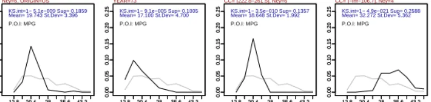
0.00 0.05 0.10 0.15 0.20 0.25 12.8 20.4 28 35.6 43.2 0.00 0.05 0.10 0.15 0.20 0.25 12.8 20.4 28 35.6 43.2 Ncy=6, ORIGIN=US KS.int=1− 5.1e−009 Sup= 0.1859 Mean= 19.743 St.Dev= 3.396 P.O.I: MPG 0.00 0.05 0.10 0.15 0.20 0.25 12.8 20.4 28 35.6 43.2 0.00 0.05 0.10 0.15 0.20 0.25 12.8 20.4 28 35.6 43.2 YEAR=73

KS.int=1− 9.1e−005 Sup= 0.1005 Mean= 17.100 St.Dev= 4.700 P.O.I: MPG 0.00 0.05 0.10 0.15 0.20 0.25 12.8 20.4 28 35.6 43.2 0.00 0.05 0.10 0.15 0.20 0.25 12.8 20.4 28 35.6 43.2 CC= (222.8−261.5], Ncy=6 KS.int=1− 3.5e−010 Sup= 0.1357 Mean= 18.648 St.Dev= 1.992 P.O.I: MPG 0.00 0.05 0.10 0.15 0.20 0.25 12.8 20.4 28 35.6 43.2 0.00 0.05 0.10 0.15 0.20 0.25 12.8 20.4 28 35.6 43.2 CC= (−inf−106.7], Ncy=4 KS.int=1− 4.9e−021 Sup= 0.2588 Mean= 32.272 St.Dev= 5.362 P.O.I: MPG

Fig. 1.Graphical representation of distribution rules for the dataset auto-mpg

Since the consequent of one distribution rule is an empirical distribution, it can be approximately represented by a frequency polygon. The rules in Figure 1 were obtained from the dataset auto-mpg [13]. The antecedent of the rule is displayed as the main title. Some selected measures of the distribution and the name of the property of interest (P.O.I.: MPG) are shown within the plot. The x axis has the domain of the P.O.I. and the y axis the estimated probability density. The distribution for the set of cases that satisfy the condition is shown in black, and thea prioridistribution for the whole population is shown in grey. The first distribution rule shown in Figure 1 tells us that cars with 6 cylinders built on the US tend to make less miles per galon than the whole set of cars. For

(5)

those cars, the values of MPG are very concentrated around 20. Nevertheless, we can see that there are some economic cars in this group because of the right tail of the black curve. The interest of this rule is shown as KS.int, the complement to 1 of the Kolmogorov-Smirnov test p-value.

3 Visual interactive discovery

Given a population and a criterion of interest, the number of interesting sub-groups/distribution rules can be very large. As in the discovery of association rules, for the data analyst to explore the discovered patterns it is useful that a post processing rule browsing environment exists.

How can a data analyst browse a large number of rules? In the case of asso-ciation rules browsing can be done through the lattice of itemsets [7]. The space of itemsets is structured using the generality relation. Traversing of the lattice can be done by fetching generalizations or specializations of a chosen rule.

In the case of distribution rules, the discrete lattice approach is not adequate since the consequent is a distribution. In that case, browsing can be done by view-ing the space of distribtuions as continuous. A simple and effective approach is to represent each distribution by statistical measures of location (mean, median and mode), spread (standard deviation) and shape (skewness and kurtosis), and structure the space of subgroups using these measures as coordinates.

We propose a visual interactive subgroup discovery procedure that graph-ically displays the distribution of each subgroup and allows the navigation by the data analyst in a chosen continuous space of subgroups. The space of sub-groups for a particular problem is represented as a two-dimensional plot, where each point is a possible subgroup. A simple example is a mean-variance plot. Each subgroup is placed on the plot according to the mean and variance of its consequent distribution. Other subgroup spaces will be median-mode, skewness-kurtosis and mean-skewness-kurtosis. Other choices can also be considered.

The two dimensional space will serve as a browsing device. The data ana-lyst can click on one of the points of that space and visualize the distributions and definitions of the corresponding subgroup or sugroups. In this phase the se-lected subgroup is also visually and statistically compared to a reference group (Algorithm 1).

Algorithm 1. Interactive subgroup discovery

1. Discover potentially interesting subgroups (all that satisfy the criterion) 2. Display the interesting subgroups in a summary 2D plot

3. Locate the region of interest in the summary plot

4. Zoom in on a particular subgroup by clicking on a point of the plot

5. Visually inspect the sub group (definition / frequency polygon / interest measures)

6. Save this subgroup if wanted 7. Stop or Go to step 3

(6)

3.1 Continuous spaces for subgroups

A continuous space of subgroups can be represented as an x-y plot, where the coordinates x and y represent statistical measures of the distribution of the property of interest.

The skewness-kurtosis space, for example, gives the data analyst an overall picture of the shapes of the distributions of the subgroups. The mean-kurtosis gives an idea of the location of the distributions as well as of how their shapes are more or less flat.

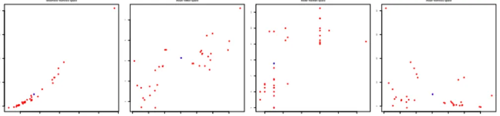
1 2 3 4 5 6 0 10 20 30 40 skewness−kurtosis space 6 7 8 9 10 11 12 3 4 5 6 7 mean−stdev space 4 6 8 10 12 14 5 6 7 8 9 10 11 mode−median space 6 7 8 9 10 11 12 0 10 20 30 40 mean−kurtosis space

Fig. 2. Four different spaces for plotting the interesting subgroups found from the

Wages dataset. The solid squares represent the whole population.

In Fig. 2 we can see the interesting subgroups found for the dataset Wages [1] represented on different spaces. On the top left we have the skewness-kurtosis space. Each subgroup is represented as a point on this space. The solid square represents thea prioridistribution (the whole population).

Skewness and kurtosis are shape measures of distributions. Skewness is re-lated to the asymetry of the distribution. It has value zero if its rigth tail is symetric to its left tail, greater than zero if its right tail is more pronounced than its left tail and less than zero otherwise. Kurtosis is related to the peaked-ness of the distribution. Intuitively, A high value of kurtosis indicates that there is a high peak, while a relatively flat distribution gets a low kurtosis. A Normal distribution has a kurtosis of 3. The “kurtosis excess” is defined as kurtosis-3, and is 0 for the Normal distribution. This is the kurtosis measure we use in this work.

Using the skewness-kurtosis plot, the data analyst has an idea of the existing shapes of the distributions and can look for distributions with particular shapes. For the subgroups in Fig. 2 we can see that the distributions have a longer right tail (skewness>0) and tend to have a relatively high kurtosis.

The mean-standard deviation space (top left of Fig. 2) identifies the sub-groups that have their mean below and above the whole population (x-axis). The y-axis gives the standard deviation. A low standard deviation indicates that a subgroup is easier to characterize and that the rule underlying it is more informa-tive. From this plot, the data analyst can, for example, identify well characterized subgroups with relatively low mean wage (bottom left of the mean-stdev space).

(7)

The mode-median space depicts the location of the distributions of the prop-erty of interest for the subgroups, both through mode and median. In this plot we can also identify distributions skewed to the right (if mode<median) or to the left (mode>median).

The fourth possibility for subgroup representation in Fig. 2 is the mean-kurtosis plot, which combines a measure of location on thex-axis with a measure of shape.

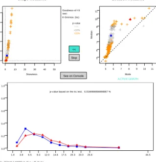
The graphical user interface developed for the prototype (Fig. 3) shows two alternative subgroup spaces (skewness-kurtosis and mode-mean in this case). Each point on the 2D plots is colored according to the Kolmogorov-Smirnov p-value of the respective subgroup. A darker cross means that the p-p-value is close to zero (<5%) and the subgroup is statistically distinct from the whole population. Lighter crosses represent subgroups whose distribtutions are statistically more similar to the whole population. The whole population is represented by the solid square.

The data analyst can choose the subgroup space to browse from (either skewness-kurtosis or mode-median). Clicking on one of the points of the chosen 2D-plot selects the respective subgroup. Its distribution for the property of in-terestWAGE(line with triangles) and description (SEX=M & MARR=Y, i.e., married males) is shown on the histogram below. The distribution of the whole popu-lation is also shown for comparison (line with squares). The selected (current) subgroup is shown as a triangle on the 2D-plots.

The process can be iterated, during which the data analyst can swap between the subgroup representation spaces. Interesting subgroups are saved for later reviewing or reporting.

4 Identifying relevant subgroups

As described above, subgroup discovery with a numerical property of interest is equated to the discovery of interesting distribution rules, i.e., rules with support and KS-interest above (or KS p-value below) given thresholds.

For distribution rule discovery we employ the algorithmCAREN-DR, based on the association rule engine CAREN [2]. CAREN-DR works by finding fre-quent itemsets not involving the property of interest y and computing their associated P.O.I. distributions on the fly. Frequent items are counted and stored in a support ascending order. For each antecedent item, a bitmap that represents its coverage is built. Antecedents are formed by depth first expansion. When an item is added to the antecedent to build a new itemset, a new bitmap is calculated (through bit-intersection) and its support can be counted through a bitcount-ing operation. To help in unfrequent itemset prunbitcount-ing durbitcount-ing itemset expansion, the algorithm builds a flat matrix with 2-itemsets counts. Thus, expensive bit-counting operations can be avoided if subsets of the candidate itemsets are not frequent.

For an efficient rule’s consequent calculation, each distribution item (the nu-meric values associated with the P.O.I.) also keeps a bitmap. Deriving a new

(8)

dis-0.0 0.2 0.4 0.6 0.8 1.0

Statisitcal Distribution of the Variable: WAGE

P ro p e rt y o f In te re s t: W A G E 1.0 3.8 6.5 9.3 12.0 14.8 17.5 20.3 23.0 25.8 44.5 5 6 7 8 9 10 11 5 6 7 8 9 10 11 Location Measures Mode M e d ia n 0 10 20 30 40 50 0 10 20 30 40 50 Shape Measures ACTIVE GRAPH Skewness K u rt o s is Goodness-of -f it test: K-Smirnov (ks) p-v alue: <5% <10% >10% >> Stop See on Console 0 10 20 30 40 50 0 10 20 30 40 50 Shape Measures Skewness K u rt o s is Goodness-of -f it test: K-Smirnov (ks) p-v alue: <5% <10% >10% 5 6 7 8 9 10 11 5 6 7 8 9 10 11 Location Measures ACTIVE GRAPH Mode M e d ia n << Stop See on Console 0.0 0.2 0.4 0.6 0.8 1.0 P ro p e rt y o f In te re s t: W A G E 1.0 3.8 6.5 9.3 12.0 14.8 17.5 20.3 23.0 25.8 44.5 S246 : AGE=(40.5-50.5] (Sup : 16.85 %)

p-v alue based on the ks test: 20.87 %

0 10 20 30 40 50 0 10 20 30 40 50 Shape Measures Skewness K u rt o s is Goodness-of -f it test: K-Smirnov (ks) p-v alue: <5% <10% >10% 5 6 7 8 9 10 11 5 6 7 8 9 10 11 Location Measures ACTIVE GRAPH Mode M e d ia n << Stop See on Console 0.0 0.2 0.4 0.6 0.8 1.0 P ro p e rt y o f In te re s t: W A G E 1.0 3.8 6.5 9.3 12.0 14.8 17.5 20.3 23.0 25.8 44.5 S254 : EDUCATION=(15.5-inf ) (Sup : 23.6 %)

p-v alue based on the ks test: 0 %

0 10 20 30 40 50 0 10 20 30 40 50 Shape Measures Skewness K u rt o s is Goodness-of -f it test: K-Smirnov (ks) p-v alue: <5% <10% >10% 5 6 7 8 9 10 11 5 6 7 8 9 10 11 Location Measures ACTIVE GRAPH Mode M e d ia n << Stop See on Console 0.0 0.2 0.4 0.6 0.8 1.0 P ro p e rt y o f In te re s t: W A G E 1.0 3.8 6.5 9.3 12.0 14.8 17.5 20.3 23.0 25.8 44.5 S247 : UNION=Y (Sup : 17.98 %)

p-v alue based on the ks test: 0 %

0 10 20 30 40 50 0 10 20 30 40 50 Shape Measures Skewness K u rt o s is Goodness-of -f it test: K-Smirnov (ks) p-v alue: <5% <10% >10% 5 6 7 8 9 10 11 5 6 7 8 9 10 11 Location Measures ACTIVE GRAPH Mode M e d ia n << Stop See on Console 0.0 0.2 0.4 0.6 0.8 1.0 P ro p e rt y o f In te re s t: W A G E 1.0 3.8 6.5 9.3 12.0 14.8 17.5 20.3 23.0 25.8 44.5

S252 : SEX=M & MARR=Y & SOUTH=N (Sup : 24.16 %)

S237 : SEX=M & MARR=Y & SECTOR=Other & RACE=white (Sup : 21.54 %) p-v alue based on the ks test: 1.11 %

S240 : SEX=M & MARR=Y (Sup : 35.21 %)

0 10 20 30 40 50 0 10 20 30 40 50 Shape Measures Skewness K u rt o s is Goodness-of -f it test: K-Smirnov (ks) p-v alue: <5% <10% >10% 5 6 7 8 9 10 11 5 6 7 8 9 10 11 Location Measures ACTIVE GRAPH Mode M e d ia n << Stop See on Console

Fig. 3.Graphical interface for interactive subgroup discovery using the wages dataset.

tribution requires intersection operations between the bitmap of the antecedent itemset and the bitmaps of the distribution items. The algorithm extracts sig-nificant rules by performing a Kolmogorov-Smirnov test between each new rule (Dy|a) and thea prioridistribution (Dy|∅).

The algorithm receives as input a minsup for antecedent filtering and anα that is used to set the maximal KS threshold.

The complexity of the algorithm is similar to the complexity of generating frequent itemsets. Experimental results with datasets of different sizes (up tp 20K records), different numbers of distinct values of the P.O.I. (up to 3842) and different minimal support thresholds (0.01 to 0.3) showed a good scale up of the algorithm [8].

5 Studying algal blooms

This subgroup discovery approach is being applied to study algae population dynamics in a river which serves as an urban water supply resource. The quantity and diversity of the algae are important for the quality of the water, which makes this an economically and socially critical eco-system.

(9)

5.1 Problem and data setup

High concentration of certain armful algae in rivers is a relevant ecological prob-lem. Blooms of these algae may reduce the life conditions in a river and cause massive deaths of fish, thus degrading water quality. The state of rivers is af-fected by toxic waste from industrial activity, farming land run-off and sewage water treatment [14]. Being able to understand and predict these blooms is there-fore very important. This problem has been studied in the MODAL project [16] (MOdels for predicting ALgal blooms in river Douro). The aim of the project is to develop tools for monitoring the quality of river water in collaboration with the local water distribution company.

We apply the visual interactive subgroup discovery approach to identify rel-evant patterns that might be useful in the description and understanding of the algae bloom processes as follows:

This methodology can be applied to the ecological data from the Modal project [16] as follows:

– By relating observable variables with posterior values of variables that are interesting to predict.

– By allowing the domain experts to inspect the subgroups.

– By showing the subgroups that apply to a given case. This allows decision support.

The data collected cover a period from 1998 to 2003 and come from the water distribution company ( ´Aguas do Douro e Paiva, S.A.), and other sources (IAREN, LPQ and University of Porto). All the attributes are continuous and can be divided in three groups:phytoplancton,chemical and physicalproperties,

andmicrobiologicalparameters.

The phytoplancton attributes record the quantity of 7 micro-algae species, Cyanobacteria, Cryptophyta, Euglenophyta, Chrysophyta, Dinophyta, Chloro-phyta and Diatom. These values were initially collected weekly and from 2002 on, biweekly.

The chemical and physical attributes record the levels of various algae nu-trients and other environmental parameters, namely, Turbidity, Temperature, PH, Alkalinity, Conductivity, Nitrates, Chlorates, Sulfates, Silica, Oxidability, Dissolved Oxygen, Iron Dissolved, Iron and Total Suspended Solids. The micro-biological attributes record the quantities of some bacteria relevant for water quality: Fecal Coliforms,Total Coliforms, Fecal Streptococcus, Sultife Reducer Clostridia, Total Germs at 22, Total Germs at 37 and Escherichia Coli. Physical-chemical and microbiological attributes had higer sampling frequency. The dataset used for subgroup discovery was obtained by pre-processing the original data as follows. For each sample of phytoplancton the values of the at-tributes were kept. For the other atat-tributes with higher sampling frequency, the values of the previous days were aggregated as maximum, minimum and mean. Attributes with the values of the previous sample the 7 phytoplancton species were also added, as well as two summary attributes measuring the Diversity and the Density of the algae. These attributes are important since a bloom of one of

(10)

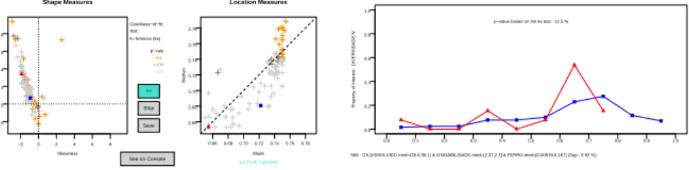
0.0 0.2 0.4 0.6 0.8 1.0

Statisitcal Distribution of the Variable: DIVERSIDADE.N

Property of Interest: DIVERSIDADE.N

0.0 0.1 0.2 0.3 0.4 0.5 0.6 0.7 0.8 0.9 1.0 0.660.680.700.720.740.760.78 0.66 0.68 0.70 0.72 0.74 0.76 0.78 Location Measures Mode Median −2 0 2 4 6 8 −2 0 2 4 6 8 Shape Measures ACTIVE GRAPH Skewness Kurtosis Goodness−of−fit test: K−Smirnov (ks) p−value: <5% <10% >10% >> Stop Save See on Console −2 0 2 4 6 8 −2 0 2 4 6 8 Shape Measures Skewness Kurtosis Goodness−of−fit test: K−Smirnov (ks) p−value: <5% <10% >10% 0.660.680.700.720.740.760.78 0.66 0.68 0.70 0.72 0.74 0.76 0.78 Location Measures ACTIVE GRAPH Mode Median << Stop Save See on Console 0.0 0.2 0.4 0.6 0.8 1.0

Property of Interest: DIVERSIDADE.N

0.0 0.1 0.2 0.3 0.4 0.5 0.6 0.7 0.8 0.9 1.0

S68 : OX.DISSOLVIDO.med=(78.4,90.1] & OXIDABILIDADE.med=(2.37,2.7] & FERRO.med=[0.00539,0.167] (Sup : 9.92 %) p−value based on the ks test: 12.5 %

−2 0 2 4 6 8 −2 0 2 4 6 8 Shape Measures Skewness Kurtosis Goodness−of−fit test: K−Smirnov (ks) p−value: <5% <10% >10% 0.660.680.700.720.740.760.78 0.66 0.68 0.70 0.72 0.74 0.76 0.78 Location Measures ACTIVE GRAPH Mode Median << Stop Save See on Console

Fig. 4.DIVERSIDADE.N is related to relatively low oxygen levels and also to relatively

low quantity of iron (FERRO).

the species is characterized by a low diversity of species and a high density of algae. Three other attributes were added: Normalized Density and Normalized Diversity (normalized versions of Density and Diversity); and BLOOM.N cal-culated as the difference between normalized density and normalized diversity. High values of BLOOM.N indicate high possibility of a bloom.

After pre-processing the data has 72 input variables, 7+5 target variables and 131 cases. In the examples below, the names of the variables appear in the original Portuguese. The results were analysed, guided and evaluated by a biologist.

5.2 Results

Choosing_DIVERSIDADE.N (normalized diversity) as the P.O.I., the mean val-ues of the the microbiology and physical-chemical parameters as explanatory variables, and with a minimum support of 0.05, we obtain 98 subgroups. Low diversity is a necessary condition for a bloom to occur. In the mode-median plot we can browse through the subgroups with lowest mode and median (left bottom corner of the plot). This is easily done by clicking on the points of the plot. One of the rules obtained relates three of the attributes: OX.DISSOLVIDO.med (mean Oxygen Dissolved), OXIDABILITY.med (mean Oxidability) and FERRO.med (mean iron), with low values of diversity (Fig. 4).

This example shows how a distribution with a relatively high Kolmogorov-Smirnov p-value can still be interesting. The distribution indicates that, for relatively low values of oxygen and low-medium values of iron there is a relatively high probability (when compared to the whole population) that the diversity is low (between 0.3 and 0.4) or very low (below 0.1). While oxygen is necessary for phytoplancton primary production, the low quantity of one nutrient (iron) may reduce the phytoplancton to the species that live well under those conditions. This situation may lead to a bloom of one of the species. In Fig. 5 we can see how, for example, the species CRIPTOFITAS lives well under such conditions.

High values of BLOOM.N may indicate algae blooms (high density of micro-algae and low diversity). With this P.O.I., 27 subgroups were found, using a minimum support of 0.05. Through the mode-median plot the data analyst iden-tifies potential bloom conditions and visualizes the corresponding distribution

(11)

0.0 0.2 0.4 0.6 0.8 1.0

Statisitcal Distribution of the Variable: CRIPTOFITAS

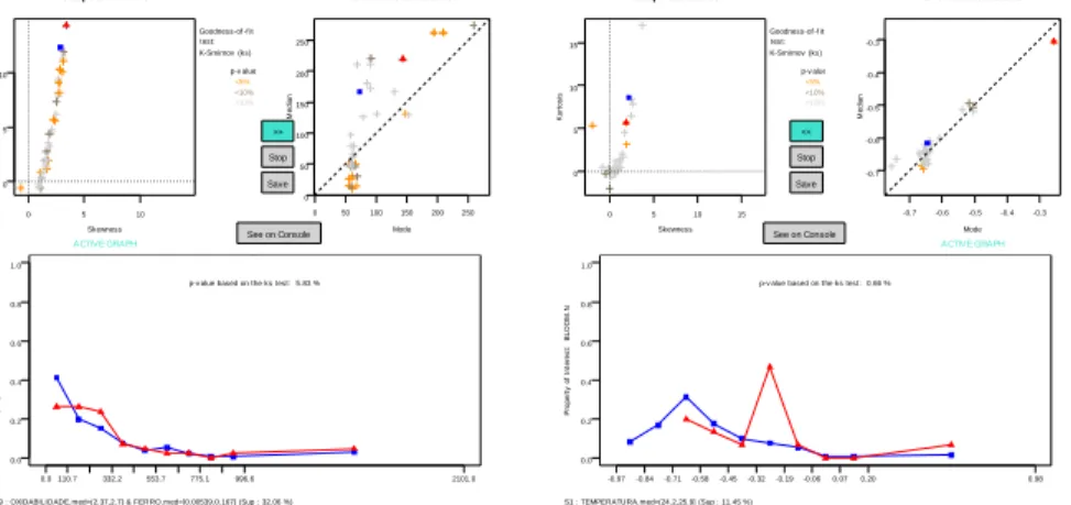
P ro p ert y o f In te re s t: C R IP T O F IT A S 0.0 110.7 332.2 553.7 775.1 996.6 2101.0 0 50 100 150 200 250 0 50 100 150 200 250 Location Measures Mode M e dia n 0 5 10 0 5 10 Shape Measures ACTIVE GRAPH Skewness K u rt o s is Goodness-of -f it test: K-Smirnov (ks) p-v alue: <5% <10% >10% >> Stop Save See on Console 0.0 0.2 0.4 0.6 0.8 1.0 P ro p ert y o f In te re s t: C R IP T O F IT A S 0.0 110.7 332.2 553.7 775.1 996.6 2101.0

S9 : OXIDABILIDADE.med=(2.37,2.7] & FERRO.med=[0.00539,0.167] (Sup : 32.06 %) p-v alue based on the ks test: 5.83 %

0 50 100 150 200 250 0 50 100 150 200 250 Location Measures Mode M e dia n 0 5 10 0 5 10 Shape Measures ACTIVE GRAPH Skewness K u rt o s is Goodness-of -f it test: K-Smirnov (ks) p-v alue: <5% <10% >10% >> Stop Save See on Console 0.0 0.2 0.4 0.6 0.8 1.0

Statisitcal Distribution of the Variable: BLOOM.N

P ro p e rt y o f In te re s t: B L O O M .N -0.97-0.84-0.71-0.58-0.45-0.32-0.19-0.060.07 0.20 0.98 -0.7 -0.6 -0.5 -0.4 -0.3 -0.7 -0.6 -0.5 -0.4 -0.3 Location Measures Mode M e dia n 0 5 10 15 0 5 10 15 Shape Measures ACTIVE GRAPH Skewness K u rt o s is Goodness-of -f it test: K-Smirnov (ks) p-v alue: <5% <10% >10% >> Stop Save See on Console 0.0 0.2 0.4 0.6 0.8 1.0 P ro p e rt y o f In te re s t: B L O O M .N -0.97-0.84-0.71-0.58-0.45-0.32-0.19-0.060.07 0.20 0.98 S23 : CLORETOS.med=(11.7,12.8] (Sup : 25.95 %)

-0.7 -0.6 -0.5 -0.4 -0.3 -0.7 -0.6 -0.5 -0.4 -0.3 Location Measures Mode M e dia n 0 5 10 15 0 5 10 15 Shape Measures ACTIVE GRAPH Skewness K u rt o s is Goodness-of -f it test: K-Smirnov (ks) p-v alue: <5% <10% >10% >> Stop Save See on Console 0.0 0.2 0.4 0.6 0.8 1.0 P ro p e rt y o f In te re s t: B L O O M .N -0.97-0.84-0.71-0.58-0.45-0.32-0.19-0.060.07 0.20 0.98 S1 : TEMPERATURA.med=(24.2,25.9] (Sup : 11.45 %)

-0.7 -0.6 -0.5 -0.4 -0.3 -0.7 -0.6 -0.5 -0.4 -0.3 Location Measures Mode M e dia n 0 5 10 15 0 5 10 15 Shape Measures ACTIVE GRAPH Skewness K u rt o s is Goodness-of -f it test: K-Smirnov (ks) p-v alue: <5% <10% >10% >> Stop Save See on Console 0.0 0.2 0.4 0.6 0.8 1.0 P ro p e rt y o f In te re s t: B L O O M .N -0.97-0.84-0.71-0.58-0.45-0.32-0.19-0.060.07 0.20 0.98

S14 : SULFATOS.med=(23.2,28.5] & FE.DISSOLVIDO.med=(0.0196,0.0295] (Sup : 10.69 %) p-v alue based on the ks test: 0.45 %

S11 : SULFATOS.med=(23.2,28.5] & CLORETOS.med=(11.7,12.8] (Sup : 7.63 %) p-v alue based on the ks test: 1.55 %

-0.7 -0.6 -0.5 -0.4 -0.3 -0.7 -0.6 -0.5 -0.4 -0.3 Location Measures Mode M e dia n 0 5 10 15 0 5 10 15 Shape Measures ACTIVE GRAPH Skewness K u rt o s is Goodness-of -f it test: K-Smirnov (ks) p-v alue: <5% <10% >10% >> Stop Save See on Console 0.0 0.2 0.4 0.6 0.8 1.0 P ro p e rt y o f In te re s t: B L O O M .N -0.97-0.84-0.71-0.58-0.45-0.32-0.19-0.060.07 0.20 0.98 S7 : SILICA.med=(4.05,4.43] (Sup : 5.34 %)

S2 : TEMPERATURA.med=(22.6,24.2] & SILICA.med=(2.89,3.28] (Sup : 12.21 %) p-v alue based on the ks test: 7.73 %

-0.7 -0.6 -0.5 -0.4 -0.3 -0.7 -0.6 -0.5 -0.4 -0.3 Location Measures Mode M e dia n 0 5 10 15 0 5 10 15 Shape Measures ACTIVE GRAPH Skewness K u rt o s is Goodness-of -f it test: K-Smirnov (ks) p-v alue: <5% <10% >10% >> Stop Save See on Console 0 5 10 15 0 5 10 15 Shape Measures Skewness K u rt o s is Goodness-of -f it test: K-Smirnov (ks) p-v alue: <5% <10% >10% -0.7 -0.6 -0.5 -0.4 -0.3 -0.7 -0.6 -0.5 -0.4 -0.3 Location Measures ACTIVE GRAPH Mode M e dia n << Stop Save See on Console 0.0 0.2 0.4 0.6 0.8 1.0 P ro p e rt y o f In te re s t: B L O O M .N -0.97-0.84-0.71-0.58-0.45-0.32-0.19-0.060.07 0.20 0.98 S1 : TEMPERATURA.med=(24.2,25.9] (Sup : 11.45 %)

0 5 10 15 0 5 10 15 Shape Measures Skewness K u rt o s is Goodness-of -f it test: K-Smirnov (ks) p-v alue: <5% <10% >10% -0.7 -0.6 -0.5 -0.4 -0.3 -0.7 -0.6 -0.5 -0.4 -0.3 Location Measures ACTIVE GRAPH Mode M e dia n << Stop Save See on Console 0.0 0.2 0.4 0.6 0.8 1.0 P ro p e rt y o f In te re s t: B L O O M .N -0.97-0.84-0.71-0.58-0.45-0.32-0.19-0.060.07 0.20 0.98 S3 : FE.DISSOLVIDO.med=(0.0295,0.0394] (Sup : 13.74 %)

0 5 10 15 0 5 10 15 Shape Measures Skewness K u rt o s is Goodness-of -f it test: K-Smirnov (ks) p-v alue: <5% <10% >10% -0.7 -0.6 -0.5 -0.4 -0.3 -0.7 -0.6 -0.5 -0.4 -0.3 Location Measures ACTIVE GRAPH Mode M e dia n << Stop Save See on Console 0.0 0.2 0.4 0.6 0.8 1.0 P ro p e rt y o f In te re s t: B L O O M .N -0.97-0.84-0.71-0.58-0.45-0.32-0.19-0.060.07 0.20 0.98

S2 : TEMPERATURA.med=(22.6,24.2] & SILICA.med=(2.89,3.28] (Sup : 12.21 %) p-v alue based on the ks test: 7.73 %

0 5 10 15 0 5 10 15 Shape Measures Skewness K u rt o s is Goodness-of -f it test: K-Smirnov (ks) p-v alue: <5% <10% >10% -0.7 -0.6 -0.5 -0.4 -0.3 -0.7 -0.6 -0.5 -0.4 -0.3 Location Measures ACTIVE GRAPH Mode M e dia n << Stop Save See on Console 0.0 0.2 0.4 0.6 0.8 1.0 P ro p e rt y o f In te re s t: B L O O M .N -0.97-0.84-0.71-0.58-0.45-0.32-0.19-0.060.07 0.20 0.98 S1 : TEMPERATURA.med=(24.2,25.9] (Sup : 11.45 %)

0 5 10 15 0 5 10 15 Shape Measures Skewness K u rt o s is Goodness-of -f it test: K-Smirnov (ks) p-v alue: <5% <10% >10% -0.7 -0.6 -0.5 -0.4 -0.3 -0.7 -0.6 -0.5 -0.4 -0.3 Location Measures ACTIVE GRAPH Mode M e dia n << Stop Save See on Console

Fig. 5. The mode-median plot helped identifying the relation between iron, oxygen

and the species CRIPTOFITA (left). At the right screen we can see that BLOOM.N is affected by relatively high temperature. This subgroup is easy to identify through the mode-median plot.

for the target variable. In Fig. ??we can see a rule that relates relatively high temperatures (around 25 degrees Celsius) with a distribution of bloom values shifted right. This is a well known effect of high temperatures, typically occurring during Summer.

5.3 Discussion

Using this prototype, the data analyst and the biologist were able to identify distributions with interesting values for the target variables. Distribution rule generation is very fast (less than 5 seconds), and moving from subgroup to sub-group is made easy by the graphical interface. The mode-median plot is a very useful browsing device for these data. Looking for extremely skewed distribu-tions of the target variables is facilitated with this subgroup space. By having immediate acces to all the generated subgroups, the data analyst can compare nearby subgroups and examine their descriptive conditions.

The display of the distribution provides information that may be hidden by a summary measure such as mean. A distribution curve with two modes, for ex-ample, may indicate that a particular subgroup has two possible outcomes (Fig. 4). If one of those outcomes is critical, than the antecedent of the subgroup may become an alarm trigger for water monitoring. This also implies that not only extreme values of median or mode indicate potentially interesting subgroups. The skewness-kurtosis plot is relatively hard to use in this application. These two measures may have values which are difficult to interpret and do not have an intuitive reading. Other measures such as maximum of the distribution and mode may provide more intuitive reading for the data analyst.

(12)

6 Related work

Kl˝osgen [10] identified the subgroup discovery data mining problem. The ex-amples shown are for categorical (and typically binary) properties of interest. Wrobel [17] proposed a multi-relational variant of categorical subgroup discovery. Gamberger et al. [5] applied subgroup discovery to the study of atheosclerotic coronary heart disease (CHD). The target is a binary class attribute (patient has/doesn’t have disease). Subgroups have the form of IF-THEN rules and are visualized by displaying the distribution of one of the independent variables (e.g., AGE), for the whole population and for some of the subgroups discovered.

Later, Gambergeret al.[4] proposed two subgroup discovery algorithms and applied them again on a CHD study. The rule discovery algorithms are inspired in beam-search. Kavseket al.[9] adapated the APRIORI association rule discovery algorithm for subgroup discovery with categorical properties of interest.

Browsing and post-processing environments for association rules discovery include PEAR [7] and Maet al.’s work [12]. These works propose browsing large sets of association rules structured as a generality lattice of itemsets.

Distribution rules are related to Quantitative Association Rules (QAR) [1], but take advantage of the whole distribution instead of specific distribution mea-sures. However, the two dimensional visual browsing space approach we present, can also be used with QAR. In this case, the representation of the subgroup would be merely textual since we would not have a subgroup distribution to display.

7 Conclusions

In this paper we have presented a visual interactive subgroup discovery approach for numerical properties of interest. Subgroups are discovered as distribution rules (DR), and an interesting subgroup corresponds to a DR with sufficient support and having a distribution for the property of interest distinct from the whole population. The similarity between distributions is measured as the Kolmogorov-Smirnov statistical test’s p-value.

A large set of subgroups is presented to a data analyst as a two dimensional plot, corresponding to a chosen space of subgroups. Each point on the plot is a different subgroup. The data analyst can inspect each of the subgroups by clicking on the respective point. Each subgroup is displayed with its set of conditions (which define the subgroup), its support, and the distribution of the property of interest.

The approach is being used in a project for monitoring the quality of water in a river. In this application, the properties of interest are the ones related with the control of algal blooms, which may affect dramatically the quality of water. The approach enables the data analyst to explore the causes for low diversity or high density of algal species.

(13)

Acknowledgments:We would like to thank Lu´ıs Torgo for comments and discussions, the biologist Dr. Catarina Magalh˜aes for domain expert guidance and evaluation of the results and Rita Ribeiro for preparing the MODAL data.

References

1. Y. Aumann and Y. Lindell. A statistical theory for quantitative association rules. Journal of Intelligent Information Systems, 2003.

2. P. J. Azevedo. CAREN - A java based apriori implementation for classification purposes. Technical report, Universidade do Minho, Departamento de Inform´atica, June 2003.

3. S. Brin, R. Motwani, J. D. Ullman, and S. Tsur. Dynamic itemset counting and implication rules for market basket data. In J. Peckham, editor, Proceedings of the 1997 ACM SIGMOD International Conference on Management of Data, pages 255–264, Tucson, Arizona, 13–15 June 1997.

4. D. Gamberger and N. Lavrac. Active subgroup mining: a case study in coronary heart disease risk group detection. Artificial Intelligence in Medicine, 28(1):27–57, 2003.

5. D. Gamberger, N. Lavrac, and D. Wettschereck. Subgroup visualization: A method and application in population screening. InProceedings of the International Work-shop on intelligent Data Analysis in Medicine and Pharmacology, IDAMAP, 2002. 6. A. Jorge. Hierarchical clustering for thematic browsing and summarization of large sets of association rules. InSIAM SDM 2004, Data Mining Conference, Orlando, Florida, April 2004.

7. A. Jorge, Po¸cas, and P. J. Azevedo. Post-processing operators for browsing large sets of association rules. In S. Lange, K. Satoh, and C. H. Smith, editors, Pro-ceedings of Discovery Science, DS 02, Luebeck, Germany, number 2534 in Lecture Notes in Computer Science, pages 414–421. Springer-Verlag, 2002.

8. A. M. Jorge, P. J. Azevedo, and F. Pereira. Distribution rules with numerical properties of interest. submitted to PKDD 06, 2006.

9. B. Kavsek, N. Lavrac, and V. Jovanoski. Apriori-sd: Adapting association rule learning to subgroup discovery. InProceedings of the fifth International Symposium on Inteligent Data Analysis, pages 230–241. Springer, 2003.

10. W. Kl˝osgen. Explora: A multipattern and multistrategy discovery assistant. In U. Fayyad, G. Piatetsky-Shapiro, P. Smyth, and R. Uthurusamy, editors,Advances in Knowledge Discovery and Data Mining. AAAI Press, Menlo Park, CA, 1996. 11. B. Liu, W. Hsu, and Y. Ma. Pruning and summarizing the discovered associations.

InKDD ’99: Proceedings of the fifth ACM SIGKDD international conference on Knowledge discovery and data mining, pages 125–134, New York, NY, USA, 1999. ACM Press.

12. Y. Ma, B. Liu, and C. K. Wong. Web for data mining: organizing and interpreting the discovered rules using the web. SIGKDD Explor. Newsl., 2(1):16–23, 2000. 13. C. J. Merz and P. Murphy. Uci repository of machine learning database.

http://www.cs.uci.edu/∼mlearn, 1996.

14. R. P. Ribeiro and L. Torgo. Predicting harmful algae blooms. In M. e. a. Pires, editor,Proceedings of Portuguese AI Conference (EPIA’03), volume 2902 ofLNAI, pages 308–312. Springer-Verlag, 2003.

15. A. Silberschatz and A. Tuzhilin. On subjective measure of interestingness in knowl-edge discovery. InKDD ’95: Proceedings of the First International Conference on Knowledge Discovery and Data Mining, pages 275–281. AAAi Press, 1995.

(14)

16. L. Torgo. Project_MODAL(_MOdels for predicting_ALgal blooms in river_Douro. http://modys.niaad.liacc.up.pt/projects/modal, 2006.

17. S. Wrobel. An algorithm for multi-relational discovery of subgroups. In J. Ko-morowski and J. Zytkow, editors,Proc. First European Symposium on Principles of Data Mining and Knowledge Discovery, PKDD’97, pages 78–87. Springer-Verlag, 1997.