Efficiently learning efficient programs

Imperial College London

Department of Computing

Efficiently learning efficient programs

Andrew Cropper

Submitted in part fulfilment of the requirements for the degree of Doctor of Philosophy in Computing of Imperial College London and

Abstract

Discovering efficient algorithms is central to computer science. In this thesis, we aim to discover efficient programs (algorithms) using machine learning. Specifically, we claim we canefficiently learn programs (Claim 1), and learn

efficientprograms (Claim 2).

In contrast to universal induction methods, which learn programs using only examples, we introduce program induction techniques which addition-ally use background knowledge to improve learning efficiency. We focus on inductive logic programming (ILP), a form of program induction which uses logic programming to represent examples, background knowledge, and learned programs.

In the first part of this thesis, we support Claim 1 by using appropriate back-ground knowledge to efficiently learn programs. Specifically, we use logical minimisation techniques to reduce the inductive bias of an ILP learner. In addi-tion, we use higher-order background knowledge to extend ILP from learning first-order programs to learning higher-order programs, including the support for higher-order predicate invention. Both contributions reduce learning times and improve predictive accuracies.

In the second part of this thesis, we support Claim 2 by introducing tech-niques to learn minimal cost logic programs. Specifically, we introduce Metaopt, an ILP system which, given sufficient training examples, is guaranteed to find minimal cost programs. We show that Metaopt can learn minimal cost robot strategies, such as quicksort, and minimal time complexity logic programs, including non-deterministic programs.

Overall, the techniques introduced in this thesis open new avenues of re-search in computer science and raise the potential for algorithm designers to discover novel efficient algorithms, for software engineers to automate the building of efficient software, and for AI researchers to machine learn efficient robot strategies.

Acknowledgements

I have been incredibility fortunate to have had Stephen Muggleton as a supervisor, and I thank him for supervising this work. Stephen’s enthusiasm for and knowledge of science has been inspiring, and I will be forever grateful to him for providing me with the most intellectually rewarding period of my life.

I thank Katsumi Inoue for acting as my host during multiple research visits to the National Institute of Informatics, and Joshua Tennebaum for acting as my host during a research visit to the Massachusetts Institute of Technology.

Declaration of originality

I declare that the work in this thesis is my own and all related other work is appropriately referenced.

Copyright declaration

The copyright of this thesis rests with the author and is made available under a Creative Commons Attribution Non-Commercial No Derivatives licence. Re-searchers are free to copy, distribute or transmit the thesis on the condition that they attribute it, that they do not use it for commercial purposes and that they do not alter, transform or build upon it. For any reuse or redistribution, researchers must make clear to others the licence terms of this work.

Contents

2.2 Logical reasoning . . . 11 2.3 Inductive inference . . . 13 2.4 Automatic programming . . . 14 2.4.1 Deductive approaches . . . 14 2.4.2 Program induction . . . 15 2.5 Machine learning . . . 16

2.5.1 Computational learning theory . . . 17

2.6 Logic programming . . . 18

2.7 Inductive logic programming . . . 18

3 Meta-interpretive learning 24 3.1 Logic programming . . . 24 3.1.1 Computation . . . 26 3.2 Meta-interpretive learning . . . 28 3.3 Metagol . . . 32 3.4 Summary . . . 35

4 Logical minimisation of metarules 36 4.1 Introduction . . . 36

4.2 Related work . . . 37

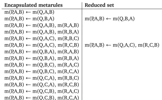
4.3 Metarules and encapsulation . . . 38

4.4 Logically reducing metarules . . . 39

4.4.1 Reduction of metarules inH₂2∗ . . . 40

4.4.2 Completeness theorem forH_m2∗ . . . 41

4.4.3 RepresentingH_m2∗programs in H₂2∗ . . . 43

4.5 Experiments . . . 44

4.5.1 Learning kinship relations . . . 45

4.5.2 Learning robot plans . . . 47

4.6 Future work . . . 49

4.7 Summary . . . 50

5 Learning higher-order programs 51 5.1 Introduction . . . 51

5.2 Related work . . . 52

5.3 Framework . . . 53

5.3.1 Abstracted MIL . . . 55

5.3.2 Language classes, expressivity, and complexity . . . 55

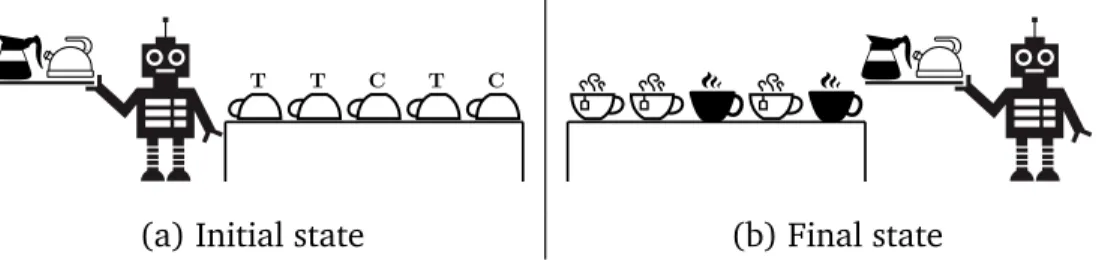
5.4 MetagolAI . . . 57 5.5 Experiments . . . 59 5.5.1 Robot waiter . . . 60 5.5.2 Chess strategy . . . 61 5.5.3 Droplast . . . 63 5.6 Future work . . . 66 5.7 Summary . . . 66 6 Metaopt 67 6.1 Introduction . . . 67

6.3 Metaopt . . . 69

6.4 Summary . . . 71

7 Learning efficient robot strategies 72 7.1 Introduction . . . 72

7.2 Related work . . . 73

7.3 Resource complexity . . . 75

7.4 Implementation . . . 76

7.5 Experiments . . . 77

7.5.1 Learning robot librarian strategies . . . 78

7.5.2 Learning robot postman strategies . . . 80

7.5.3 Learning robot sorting strategies . . . 82

7.6 Future work . . . 84

7.7 Summary . . . 85

8 Learning efficient logic programs 86 8.1 Introduction . . . 86

8.2 Related work . . . 87

8.3 Framework . . . 88

8.4 Implementation . . . 88

8.5 Experiments . . . 89

8.5.1 Experiment 1: convergence on minimal cost programs . 89 8.5.2 Experiment 2: comparison with other systems . . . 91

8.5.3 Experiment 3: string transformations . . . 92

8.6 Future work . . . 95

8.7 Summary . . . 95

9 Conclusions and future work 97 9.1 Conclusions . . . 97 9.2 Future work . . . 99 9.2.1 Background knowledge . . . 99 9.2.2 Efficient programs . . . 102 9.2.3 Meta-interpretive learning . . . 103 9.3 Summary . . . 105

Chapter 1

Introduction

Discovering efficient algorithms is central to computer science, as illustrated by the major open problems in the field[12, 40, 30]. In this thesis, we aim to discover efficient programs (algorithms) using machine learning. Specifically, we claim:

• Claim 1: we canefficiently machine learn programs • Claim 2: we can machine learnefficientprograms

Program induction

Machine learning programs from data is calledprogram induction. The aim is to learn a program that models a set of examples. For instance, consider the following examples written as Prolog facts1_{, where the first argument is the}

input and the second is the output: f([m,a,c,h,i,n,e],e).

f([l,e,a,r,n,i,n,g],g). f([a,l,g,o,r,i,t,h,m],m).

Given these examples and background predicateshead/2,tail/2, andempty/1, a program induction system could learn a program that finds the last element of the input list, such as:

f(A,B):-head(A,B),tail(A,C),empty(C). f(A,B):-tail(A,C),f(C,B).

A program induction system should learn more accurate programs given more examples.

Efficientlylearning programs

The idea of machine learning goes back to Turing[134]who anticipated the difficulty in programming a computer with human intelligence and instead suggested building computers that learn similar to how a human child learns. Turing also suggested learning with background knowledge, and hinted at the difficultly of learning without it [88]. In contrast to universal induction methods[123, 124, 70], which induce programs only from examples, program induction systems use background knowledge to improve learning efficiency. In the above example, the background knowledge contains definitions for the predicates head/2, tail/2, and empty/1. Because they assume background knowledge, program induction approaches are less general than universal induction methods, but are more practical because the background knowledge is a form of inductive bias [81]which restricts the hypothesis space. Given no background knowledge, and thus no inductive bias, program induction methods are equivalent to universal induction methods. In the first part of this thesis (Chapters 4 and 5), we support Claim 1 by using appropriate background knowledge to efficiently learn programs.

Learningefficientprograms

Consider the following examples: f([l,o,g,i,c,a,l],l).

f([i,n,d,u,c,t,i,v,e],i). f([l,e,a,r,n,i,n,g],n).

Given these examples and background predicateshead/2,tail/2, member/2, andmsort/22, a program induction system could learn a program that finds the duplicate in the input list. Two such programs are:

Example 1 (Program 1)

f(A,B):-head(A,B),tail(A,C),member(B,C). f(A,B):-tail(A,C),f(C,B). Example 2 (Program 2) f(A,B):-msort(A,C),f1(C,B). f1(A,B):-head(A,B),tail(A,C),head(C,B). f1(A,B):-tail(A,C),f1(C,B).

Although the programs give the same result3, they differ in efficiency. Program 1 goes through the elements of the list in turn checking whether the same element exists in the rest of the list with time complexityO(n2). By contrast, Program 2

first sorts the list and then goes through checking whether any adjacent elements are the same with time complexityO(nlogn). Although textually larger, both in the number of clauses and literals, Program 2 is more efficient than Program 1. However, existing program induction approaches[123, 124, 70, 92, 87, 97] cannot distinguish between the efficiencies of programs, and instead learn textually simple programs. As the above example shows, smaller programs are not necessarily more efficient than larger ones. In the second part of this thesis (Chapters 6, 7 and 8), we address this limitation and support Claim 2 by introducing techniques to learn efficient programs.

Inductive logic programming

We introduce program induction techniques based on inductive logic program-ming (ILP)[86], a form of machine learning that uses logic programming to represent examples, background knowledge, and learned programs. Existing ILP approaches[92, 87, 97, 106]cannot distinguish between the efficiencies of programs and instead rely on an Occamist bias to learn textually simple pro-grams, such as those with the fewest literals[67]or clauses[97]. For instance, Golem[92]and Progol[87]could both learn sorting algorithms from examples, but when given background knowledge suitable for learning quicksort, both systems learned variants of insertion sort because the program was smaller and there was no bias for learning more efficient algorithms. By contrast, in Chap-ter 6, we introduce Metaopt, an ILP system biased towards learning efficient programs.

Meta-interpretive learning

We focus on meta-interpretive learning (MIL)[96, 97, 23, 25, 24], a form of ILP based on a Prolog interpreter. In contrast to a standard Prolog meta-interpreter, which tries to prove a goal by fetching first-order clauses whose heads unify with the goal, a MIL learner additionally attempts to prove a goal by fetching higher-order clauses, called metarules, whose heads unify with the goal. The resulting meta-substitutions are saved and can be reused in later proofs. Following the proof of a set of goals, a logic program is formed by projecting the meta-substitutions onto their corresponding metarules, allowing for a form of ILP which supports predicate invention and learning recursive programs, both long-standing challenges in ILP [94]. We contribute to the theory and implementation of MIL.

1.1

Contributions

To support Claims 1 and 2, we make the following contributions:

Efficiently learning programs (Claim 1)

Contribution 1: metarules Program induction systems use background knowl-edge to restrict the hypothesis space. A MIL learner takes metarules as part of the background knowledge. Metarules are a form of declarative bias [98, 108] that determine the structure of learnable programs which in turn defines the hypothesis space. Selecting which metarules to use is a trade-off between effi-ciency and expressivity: the hypothesis space increases given more metarules

[72], so we wish to use fewer metarules, but if we use too few metarules then we lose expressivity. In Chapter 4, we make these contributions to this problem:

• We use Plotkin’s clausal theory reduction algorithm [103] to logically reduce sets of metarules.

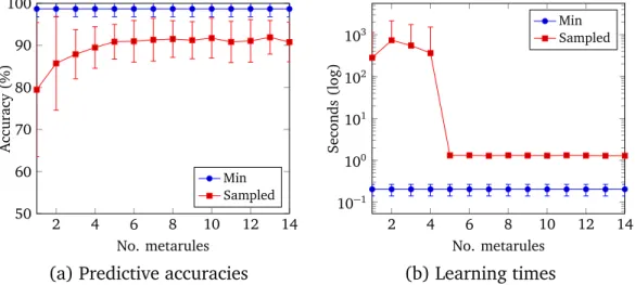
• We show that when this approach is applied to a finite hypothesis language, only two metarules are necessary to entail all hypotheses in that language. • We conduct experiments which show that, compared to learning with

non-minimal sets of metarules, learning with minimal sets of metarules improves predictive accuracies and reduces learning times.

Contribution 2: higher-order programs Compared to other forms of ma-chine learning, an advantage of using ILP for program induction is its ability to learn first-order programs[86], which are intrinsically more expressive than propositional programs. In Chapter 5, we extend ILP to support learning higher-order programs by allowing a MIL learner to use higher-higher-order definitions as background knowledge. We show that learning higher-order programs can re-duce the textual complexity required to express target classes of programs which in turn reduces the hypothesis space. We introduce Metagol_AI, a MIL learner which supports learning higher-order programs and higher-order predicate invention, such as inventing predicates for use in the higher-order abstractions

map/3andreduce/4. Overall, we make these contributions:

• We define higher-orderdefinitions,abstractions, andinventions.

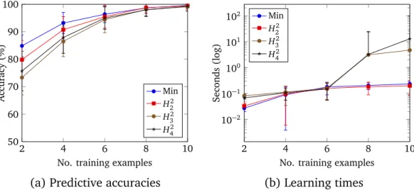
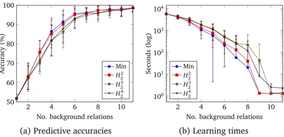
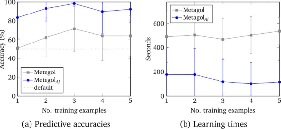
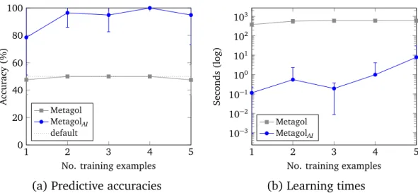
• We provide sample complexity results which show that learning higher-order programs can reduce (1) learning times, and (2) the number of examples required to reach high predictive accuracies.

• We introduce Metagol_AI, a MIL learner which supports learning higher-order programs and higher-higher-order predicate invention.

• We conduct experiments which show that, compared to learning first-order programs, learning higher-first-order programs can improve predictive accuracies by up to 50% and reduce learning times by four orders of magnitude.

This work is the first to demonstrate higher-order predicate invention and the efficiency and accuracy advantages of using higher-order abstractions[25].

Learning efficient programs (Claim 2)

Contribution 3: cost minimisation problem When learning programs from data, we should aim to learn efficient programs. However, as mentioned, existing program induction systems cannot distinguish between the efficiencies of programs. In Chapter 6, we make these contributions to this problem:

• We introduce the cost minimisation problem, a general framework for learning efficient programs.

• We introduce Metaopt, a MIL learner which solves the cost minimisation problem using a new search procedure called iterative descent.

• We prove that, given sufficient training examples, Metaopt converges on minimal cost programs.

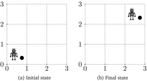
Contribution 4: learning efficient robot strategies In Chapter 7, we use Metaopt to learn efficientresource complexityrobot strategies[24]. In contrast to traditional AI planning[114], which involves the generation of a plan as a sequence of actions transforming a particular initial state to a particular final state, a strategy can be viewed as a potentially infinite set of plans, applicable to a class of initial/final state pairs[24]. Specifically, we make these contributions: • We introduce the resource complexity minimisation problem, a variant of the cost minimisation problem, where resource complexity is a user-defined measure of the efficiency of a robot strategy.

• We conduct experiments on learning robot librarian, postman, and sorter strategies which show that Metaopt learns minimal resource complexity strategies in all cases.

This work is the first to demonstrate learning efficient robot strategies[24].

Contribution 5: learning efficient logic programs

In Chapter 8, we use Metaopt to learn efficient time complexity logic programs. Specifically, we make these contributions:

• We introducetree complexity, a program cost function based on the size of a SLD-tree at the point of which a goal is proved by a logic program. • We introduce thetree complexityminimisation problem, a variant of the

cost minimisation problem.

• We conduct experiments on programming puzzles and real-world string transformation problems which show that Metaopt learns minimal tree complexity programs, including non-deterministic programs, which cor-respond to minimal time complexity programs.

1.2

Publications

We have published parts of this thesis:

• Parts of Chapter 4 appeared in [23]. I contributed (1) parts of the the-oretical framework, in particular the work on the logical reduction of metarules, (2) by conducting the experiments, and (3) by writing half of the paper.

• Parts of Chapter 5 appeared in[25]. I contributed (1) the idea of learn-ing higher-order programs, (2) the implementation MetagolAI, (3) by

conducting the experiments, and (3) by writing two-thirds of the paper. • Parts of Chapters 6 and 7 appeared in[24]. I contributed (1) the idea of learning efficient robot strategies, (2) the implementation MetagolO, (3)

by conducting the experiments, and (3) by writing half of the paper. • Parts of Chapter 6 and 8 appeared in[27]. I contributed almost all of the

work for this paper.

We have also published papers related to this thesis [28, 22, 36].

1.3

Outline

The first part of the thesis (Chapters 4 and 5) focuses on Claim 1 and introduces techniques to efficiently learn programs. The second part of this thesis (Chapters 6, 7, and 8) focuses on Claim 2 and introduces techniques to learn efficient programs. Chapters 4, 5, 6 and 7 each include a discussion of related work specific to that chapter and a brief summary. The rest of this thesis is organised as follows:

Chapter 2: Related work We discuss related work, including algorithms and computation, inductive inference, and program induction.

Chapter 3: Meta-interpretive learning We describe MIL and prerequisite con-cepts from logic programming and ILP.

Chapter 4: Logical minimisation of metarules We describe work on improv-ing the efficiency of a MIL learner by reducimprov-ing the number of metarules required.

Chapter 5: Learning higher-order programs We describe work on improv-ing the efficiency of a MIL learner by introducimprov-ing techniques to learn higher-order programs.

Chapter 6: Metaopt We introduce thecost minimisation problem, a general framework for learning efficient programs and Metaopt, a MIL learner which solves the problem.

Chapter 7: Learning efficient robot strategies We describe work on learn-ing robot strategies with minimal resource complexity.

Chapter 8: Learning efficient logic programs We describe work on learning logic programs with minimal tree complexity and thus minimal time complexity.

Chapter 9: Conclusions We conclude the thesis and discuss future work.

1.4

Summary

In this chapter, we have stated that the goal of this thesis is to machine learn programs (algorithms) from data, which we call program induction. We have highlighted that existing approaches cannot learn efficient programs. By con-trast, we have claimed we can (1) efficiently learn programs, and (2) learn

efficientprograms. We have outlined the contributions of the thesis, namely (1) the introduction of techniques to improve learning efficiency by using appro-priate background knowledge, and (2) the introduction of the first algorithm that learns efficient programs. In the next chapter, we cover related literature for the rest of the thesis, including overviews of algorithms, computation, and inductive inference.

Chapter 2

Related work

In this chapter, we detail work related to the thesis, including work on algo-rithms, computation, inductive inference, program induction, and ILP.

2.1

Algorithms and computation

Informally, an algorithm is a sequence of precise instructions to perform a task. Computation is the process of applying an algorithm to some input. Although mathematicians have studied algorithms for millennia, it was not until the 1930s that the concept of an algorithm was formalised mathematically.

In 1928, Hilbert proposed theEntscheidungsproblem[49], which asks whether there exists an ‘effectively calculable’ procedure (an algorithm) that determines whether a statement in first-order-logic is provable using the rules of logic. Before the question could be answered, the notion of an algorithm had to be formally defined, which was done independently by three logicians. Godel proposed ‘general recursive functions’ [61], Church proposedλ-definability based on hisλ-calculus[17], and Turing proposed theoretical machines, now called Turing machines[135].

Turing showed[135]that these three models were equivalent, i.e. a function is general recursive if and only if it isλ-computable if and only if it is computable on a Turing machine. The connection between the informal and formal notions of algorithm is called the Church-Turing thesis[121], which states that a function is computable by a human following an algorithm, ignoring resource limitations, if and only if it is computable by a Turing machine.

the Entscheidungsproblem was given by Church[16]who demonstrated the existence of uncomputable functions in hisλ-calculus, and by Turing[135]who showed there cannot exist a general method that decides whether any Turing machine halts, known as the halting problem.

Turing Machines

A Turing machine[135]is a hypothetical machine. It has an infinite tape divided into cells, where the tape acts as memory. Initially the tape contains only the input string and is blank everywhere else. The machine has a tape head that performs three operations: (1) read the symbol on the cell under the head, (2) edit the symbol by writing a new symbol or erasing it, (3) move the tape left or right by one cell. The choice of operation depends on a set of user-specified instructions. The machine continues to execute instructions or halts. A universal Turing machine (UTM) is a Turing machine that can simulate any Turing machine. When a programming language can do what a Turing machine can do, that language is called Turing complete. If a problem is solvable in a Turing complete language then it is solvable in all such languages.

Algorithm efficiency

A decidable function can always be computed on a Turing machine (or an equiv-alent model) given sufficient resources. However, a decidable function may not necessarily be computed efficiently. Algorithm efficiency refers to the resources required by an algorithm to compute a function. Two common[121]resource measures are (1) time complexity, which measures how long an algorithm takes to compute a function, and (2) space complexity, which measures how much memory an algorithm needs to compute a function. Efficiency is measured as a function of the length of the string representing the input. Worst-case analysis measures the maximum resources used on all inputs of a particular length. Average-case complexity measures the average resources used on all inputs of a particular length. The exact resources required by an algorithm is often difficult to establish. For example, different programming languages may influence the running time of an algorithm. Therefore, we approximate efficiency using asymptotic analysis[121], which measures the efficiency of an algorithm as the input length grows. This approximation only considers the highest order term in an expression of the cost of an algorithm, because the

highest order term dominates the other terms in the limit. For example, the function f(n) =n3+2n2+5x+10 is asymptotically at mostn3written as 0(n3).

Kolmogorov complexity

Algorithmic information theory[15]studies the resources required to represent strings. For example, consider these two strings:

00000000000000000000 10110100110000000011

Whilst the first string has the short description “twenty zeros”, the second string has no obviously simpler description than the string itself. Kolmogorov complexity [62] measures the resources needed to specify a string x as the shortest program that computesx. The shortest program is typically interpreted as the shortest Turing machine. Kolmogorov complexity is used in inductive inference and machine learning to measure the resources required to represent algorithms.

2.2

Logical reasoning

In this thesis, we aim to learn programs from data, which can be seen as deriving conclusions (programs) from premises (data). Logical reasoning uses formal logic to derive conclusions from premises, where conclusions and premises are formed of rules or facts. Two key concepts in logic are soundness and completeness[99]. A logical system is sound if and only if its inference rules prove only formulas that are valid with respect to its semantics, i.e. soundness is the property of being able to only prove true things. A logical system is complete if and only if all valid formula can be derived from the axioms and the inference rules, i.e. completeness is the property of being able to prove all true things.

We use techniques that combine the three major forms of logical reasoning: deduction, induction, and abduction [102].

Deduction Deduction is the process of deriving facts from premises formed of rules and facts. For example, consider these two statements:

mortal(A)← man(A) man(socrates)

Given these statements, we can use the implication elimination rule of deduction to derive the fact mor t al(soc r at es). In deductive reasoning, if all premises

are true and the rules of deduction are followed, then derived conclusions are necessarily true. Godel showed[86]that a small set of inference rules is complete for deriving all consequences of formulae in first-order-logic. Later, Robinson demonstrated [113]that a single rule of inference, called resolution, is sound and complete for finding refutations of statements in clausal form (Section 3.1).

Abduction Abduction seeks to explain observations and, as with deduction, is the process of deriving facts from rules and facts. For example, consider these two statements:

mortal(A)← man(A) mortal(socrates)

To explain the factmor t al(soc r at es)we could abduce the fact man(soc r at es). However, unlike deductive reasoning, abductive reasoning derives conclusions which are not guaranteed to be correct. In this example, the factman(soc r at es)

is not necessarily true.

Induction Induction is the process of forming rules from examples, and is the goal of this thesis. For example, consider these two statements:

man(socrates) mortal(socrates)

Using induction, we could form the rule that all men are mortal: mortal(A)← man(A)

We could also form the rule that all things mortal are men: man(A) ←mortal(A)

Conclusions formed in inductive reasoning are not logically valid, i.e. induced rules may be incorrect.

Inducing rules from data is theinduction problem. The induction problem has a long history in philosophy. Epicurus noted that there typically exist many hypotheses consistent with the data[52]. For example, we can form multiple rules from the two facts above about Socrates. Logically, we cannot use the data to rule out any of these hypotheses; they must all be kept as potential explanations. This notion of keeping all consistent hypotheses is known as Epicurus’s principle of multiple explanations. In practice, however, we often want to select one hypothesis, or at least exclude certain hypotheses. Occam’s principle (often called razor because it shaves away unnecessary assumptions), suggests that amongst all hypotheses consistent with the data, the simplest is the most likely[52]. For example, consider the number sequence 1, 3, 5, 7. Suppose that nrepresents the position in the sequence, then one hypothesis to describe this sequence is the expression (2n)−1, where the next number is 9. An alternative hypothesis is the expression 2n−1+ (n−1)(n−2)(n−3)(n−4), where the next number is 33. Although both hypotheses are valid, Occam’s principle says prefer the former to the latter because it is simpler. Many learning algorithms [123, 124, 97, 70] rely on an Occamist bias to decide between hypotheses.

2.3

Inductive inference

Solomonoff induction

Solomonoff’s universal inductive inference[123, 124]is a solution to the induc-tion problem. It combines Epicurus’ and Occam’s principles in a probabilistic way using Bayes’ theorem[81], represents hypotheses as Turing machines, and uses Kolmogorov complexity as a prior. The idea is that given data E, one way to find a hypothesisH (a Turing machine) that generatedE is to try all possible hypotheses on a UTM. To adhere to Occam’s principle, Solomonoff induction as-signs a prior probability to each hypothesis based on its Kolmogorov complexity. However, Solomonoff induction is incomputable because it tries every possible hypothesis, some of which will run forever. Because of the Halting problem, we cannot determine beforehand that any of the hypotheses will not terminate

Levin search

Levin’s universal search [70] is another solution to the induction problem. Similar to Solomonoff induction, Levin search tries all possible hypotheses on a UTM. The key difference is that Levin search allocates each program ptime equal to 2l(p)_{, where l(p)is the size of the program in bits. If nothing else is}

known about the problem except the observations and assuming the solution can be verified in polynomial time, Levin search is the asymptotically fastest way of finding a program to solve the problem. The algorithm has the property that the total time taken to find a solution is O(t), where t is the time used by fastest program p to compute the solution. The search time of the whole process is at most a constant factor larger than t. However, this constant is 2l(p)_,

making Levin search impractical.

2.4

Automatic programming

Automatic programming is the automatic generation of a computer program to perform a task. Universal induction methods, such as Solomonoff induction and Levin search, are forms of automatic programming. However, universal methods are impractical because they only take examples as input. Other approaches take additional information to improve efficiency.

2.4.1

Deductive approaches

Deductive approaches[77] to automatic programming build programs from full specifications, where a specification precisely states the requirements and behaviour of the desired program. For example, to build a program that returns the last element of a non-empty list, we could provide a formal specification written in Z notation[125]:

last : seq_0 X --> X

forall s : seq_0 X last s = s(#s)

Deductive approaches also take informal full specifications, such as a specifica-tion written as a Prolog program:

last([A]).

A drawback of deductive approaches is that formulating a specification is hard and typically requires a domain expert. In fact, formulating a specification can be as hard as finding a solution. For example, formulating the specification for the following string transformations is non-trivial:

`[email protected]' => `Alan Turing'

`[email protected]' => `Alonzo Church' `[email protected]' => `Kurt Godel'

2.4.2

Program induction

Deductive approaches take full specifications as input and are efficient at build-ing programs. Universal induction methods take only examples as input and are inefficient at building programs. We focus on the area between these which we callprogram induction– also called inductive programming[47], programming by example[71], and inductive program synthesis[104].

Similar to universal induction methods, program induction systems learn programs from incomplete specifications, typically input/output examples. In contrast to universal induction methods, program induction systems use back-ground knowledge, and are thus less general than universal methods, but are more practical because the background knowledge is a form of inductive bias

[81]which restricts the hypothesis space. When given no background knowl-edge, and thus no inductive bias, program induction methods are equivalent to universal induction methods.

Early work on program induction includes Plotkin on least generalisation

[103], Vere on induction algorithms for predicate calculus[137], and Summers on inducing Lisp programs [130]. Interest in program induction has grown recently, partly due to applications in real-world problems, such as end-user programming[45]and computer education [46].

We can classify program induction approaches as either task-specific or general-purpose. Task-specific approaches focus on a specific domain and are often restricted to specific data types, such as numbers[120]and strings

[44, 141]. By contrast, general-purpose systems work on many domains, but are typically less efficient. MagicHaskeller [55] is a general-purpose system that learns Haskell functions by instantiating higher-order functions from a pre-defined vocabulary. Igor2 [60]also learns recursive Haskell programs and supports auxiliary function invention but is restricted because it requires the firstkexamples of a target theory to generalise over a whole class. Esher[3]

learns recursive programs but needs to ask an oracle for examples each time a recursive call is encountered. In contrast to these approaches, this thesis is based on MIL, a general form of program induction which learns recursive Prolog programs from examples and background knowledge.

2.5

Machine learning

Program induction has been studied in many areas of machine learning, such as inductive logic programming[86], genetic programming[140], and deep learning [143]. The goal of machine learning is to develop algorithms that improve their performance over time through experience. Mitchell[81]defines machine learning as:

Definition 1 (Machine learning)A learning algorithm is said to learn from experience E with respect to some class of tasksT and performance measureP, if its performance at tasks in T, as measured byP, improves with experience E. Experience E refers to examples. Performance measure P typically measures predictive accuracy on unseen examples but is only one criterion of performance. Michie[80]suggested three performance criteria. Theweakcriterion measures how well the learned program performs on unseen data (predictive accuracy). The strong criterion additionally requires that the program is readable by a human. Finally, theultra-strongcriterion additionally requires that a human can understand and draw consequences from the program. Most forms of machine learning only support the weak criterion because the learned hypotheses are largely incomprehensible to a human, such as the hyperplanes learned by a support vector machine. By contrast, the hypotheses in program induction are computer programs, which can be read and understood by a human. Declarative forms of program induction, in which the induced programs express the logic of a computation without describing its control flow [73], such as ILP, are particularly suited for human interpretability.

We can broadly classify machine learning approaches by the type of examples (experience) available. The three common classifications are[81]: supervised learning, unsupervised learning, and semi-supervised learning. In supervised learning the task is to learn a function that generalises from labelled examples to unlabelled examples. In unsupervised learning the task is to learn how unlabelled data is organised. Semi-supervised learning is a mix of supervised

and unsupervised learning, where the examples are labelled and unlabelled. Program induction typically focuses on supervised learning.

2.5.1

Computational learning theory

Computational learning theory studies what can be learned efficiently. Two key criteria of learning efficiency are[81]:

Definition 2 (Sample complexity)Sample complexity is the number of exam-ples an algorithm needs to successfully learn a correct hypothesis.

Definition 3 (Time complexity). Time complexity is the time an algorithm needs to successfully learn a correct hypothesis.

We use both criteria throughout this thesis, but because we can measure the time complexity of a learning algorithm in the same way as any other algorithm (Section 2.1), this section focuses on sample complexity.

In the above definitions, the termsuccessfullyis vague. What does it mean for a learning algorithm to successfully learn a hypothesis? Two theories have tried to answer this question.

In Gold’s theory oflanguage identification in the limit [43], a learning al-gorithm reads an infinite sequence of examples one by one and is said to successfully identify a language in the limit if and only if after a certain number of examples the algorithm chooses the correct hypothesis and does not change this hypothesis as more examples are provided. Two drawbacks of Gold’s theory are (1) it represents an all-or-nothing approach to learning, where a hypothesis must be totally correct with respect to all the seen examples, and (2) it gives little indication of how many examples are required to converge on the correct hypothesis[99].

In contrast to Gold’s theory, Valiant’s theory of probably approximately correct learning (PAC)[136]is concerned with approximations of learnability. In Valiant’s theory, a learning algorithm PAC-identifies a concept if and only if it learns with high probability (1−δ) a hypothesis that is approximately consistent (1−ε) with the examples. This theory gives a looser definition of successfully learning a concept, which is usually considered to be a better model in machine learning[99].

These two theories define when a learning algorithm successfully learns a hypothesis, but neither tells us how many examples are required to do so. Using

PAC-learning, Blumer[9]showed that as a hypothesis space grows, you need more examples to PAC-learn a hypothesis. The result, known as the Blumer bound, implies that given two hypothesis spaces which (1) both contain a target hypothesis, and (2) are of different sizes, then searching the smaller hypothesis space will reduce learning times and improve predictive accuracies compared to searching the larger hypothesis space. The idea of reducing a hypothesis space without excluding the target hypothesis is the focus of Chapters 4 and 5. We formally describe the Blumer bound in Chapter 3.

2.6

Logic programming

Logic has long been viewed as central to achieving AI[134, 78]. Logic program-ming[129, 74]is a form of declarative programming[73]based on formal logic. In contrast to imperative programming, which views a program as a sequence of step-by-step instructions (a procedure), logic programming views a program as a logical theory, where computation is viewed as finding a proof of the theory (program). A search for a proof is based on deductive reasoning, specifically Robinson’s resolution principle[113], a single rule of deductive inference which is refutation complete for theories in clausal form. Resolution takes as input a clausal theory P and a goal G and tries to derive the empty clause, which represents falsity. To improve efficiency, Kowalski introduced SLD-resolution

[63], which is sound and complete for a restricted form of a logic called Horn logic. Although restricted, Horn logic is Turing complete[132]. Prolog, a popu-lar logic programming language, is based on Horn logic – although contains extra-logical features, such as cuts. We detail logic programming in Section 3.1.

2.7

Inductive logic programming

ILP is a form of machine learning that uses logic programming to represent examples, background knowledge, and induced hypotheses (programs). We use thelearning from entailmentsetting of ILP[93], where an example corresponds to an observation about the truth or falsity of a formula F and a hypothesisH

covers F ifH entails F (H_|=F). Two other learning settings are (1)learning from interpretations[7], where an example is a logical interpretation I and an example is covered by a hypothesis H if I is a model forH, and (2) learning from proofs[101], where an example is a proof P and a hypothesis H covers an

example ifP is a proof of the hypothesisH. Learning from proofs in ILP is similar to learning programs from execution traces[66], which some researchers view as program induction[112]. However, proofs and interpretations carry more in-formation than examples and are therefore easier to learn from[94]. Therefore, such approaches should be distinguished from learning from examples.

An advantage of using ILP over other forms of machine learning is that, because of the expressivity of logic (Horn logic is Turing complete[132]), ILP systems can learn complex relational theories, such as solutions to the Michalski trains problem[65]. By contrast, most other forms of machine learning, such a neural networks [69], are restricted to finite, propositional, feature-based representations of examples and concepts, and thus struggle to learn complex relational theories.

Another advantage of ILP is that because hypotheses are logic programs, they can be read by humans, potentially supporting Michie’sstrongandultra-strong

criteria of learning, which is not the case in many other learning approaches

[94].

Predicate invention Predicate invention has been repeatedly stated as an important challenge in ILP[90, 128, 94]. The idea behind predicate invention is for an ILP system to introduce new predicates to improve learning performance. In program induction, predicate invention can be seen as inventing auxiliary functions, as one does when manually writing a program, for example to reduce code duplication or to improve the readability of a program. Popular ILP systems, such as FOIL[106], Progol[87], and ALEPH[127], do not support predicate invention, nor do most program induction systems. Meta-level abduction[53] uses abduction and meta-level reasoning to invent predicates that represent propositions. By contrast, MIL, on which this thesis is based, uses abduction to invent predicates representing relations, i.e. relations which are not in the initial background knowledge nor in the examples. For instance, in[97], MIL invented a predicate corresponding the parent relation when learning a grandparent relation. In chapter 5, we extend MIL and the associated Metagol implementation to support order predicate invention for use in higher-order constructs, such asmap/3,reduce/3, andfold/5.

Recursion Recursion is fundamental to computer science and algorithms[2], yet it has been difficult for ILP to learn recursive programs[94]– which is also the case for program induction in general (Section 2.4.2). The ATRE system

was used to learn a recursive ontology theory from biological text[76]and to learn recursive patterns from biomedical text[5]. However, ARTE cannot easily be extended to learn general programs from examples[28]. Moreover, ARTE was not shown to learn recursive theories from small numbers of examples

[28]. By contrast, MIL supports learning general recursive programs, such as learning definite clause grammars and recursive definitions for the concept of a staircase[97]. In this thesis, we further demonstrate the ability of MIL to learn general recursive programs from small numbers of examples, such as learning robot strategies for quicksort (Chapter 7) and to learn efficient time complexity programs to find duplicate elements in a list (Chapter 8).

Higher-order logic McCarthy[79]and Lloyd[75]advocated using higher-order logic to represent knowledge. Similarly, in [94], the authors argued that using higher-order representations in ILP provide more flexible ways of representing background knowledge.

MIL uses higher-order metarules and a meta-interpreter (which is intrinsi-cally higher-order) to learn programs from examples. Metarules are a form of declarative bias [98, 108]. In contrast to other forms of declarative bias in ILP, such as modes[87, 127]or grammars[20], metarules are logical statements that can be reasoned about. Metarules were introduced in the Blip system

[35], who used similar metarules to us, such transitivity (chain) and converse (inverse) metarules. Metarules are also called second-order schemata[109].

In[57], the authors explore generality measures for metarules, which they call rule schemas, in their RDT system. A generality order is necessary be-cause the RDT system searches the hypothesis space (which is defined by the metarules) in a top-down general-to-specific order. A key difference between RDT and MIL is that whereas RDT requires metarules of increasing complexity (e.g. rules with an increasing number literals in the body), MIL derives more complex metarules through predicate invention.

Determining which metarules are necessary to learn certain classes of pro-grams has yet to be explored. In Chapter 4, we address this issue by using logical reduction techniques to find logically minimal sets of metarules, which improves predictive accuracies and lowers learning times, and we show that in some cases only two metarules are needed to derive a whole class of metarules Although learning higher-order programs has been considered in program induction[60, 55], it has been under explored in ILP. In Chapter 5, we extend MIL from learning first-order programs to learning higher-order programs,

which improves predictive accuracies and lowers learning times.

ILP systems In this thesis, we develop Metagol, an ILP system based on the MIL framework. It is difficult to directly compare Metagol to other ILP systems. For instance, some notable ILP systems, such as MIS[119]and CIGOL[90]are interactive, i.e. they require input from a user during the learning, whereas Metagol does not.

As described above, Metagol supports predicate invention, the automatic introduction of new predicate symbols, which has long been a challenge for ILP[90, 128, 94] and which most ILP systems do not support[119, 106, 92, 87, 127, 111, 21, 67]. Systems that do support predicate invention support different levels of predicate invention. For instance, Cigol[90]only introduces new predicates when a negative example is confirmed by an oracle (i.e. Cigol is an interactive system). By contrast, Metagol automatically introduces new predicate symbols without the need for negative examples. In addition, ASPAL

[4]and INSPIRE[118]both support predicate invention, but both are yet to demonstrate nested predicate, which is frequently demonstrated in this thesis using Metagol.

In many of our experiments, we learn explicitly recursive programs (i.e. programs where the recursion is not hidden in the background knowledge), such as in Chapter 8 where we use Metagol to learn an efficient and recur-sive programs to find a duplicate element in a list. Many ILP systems cannot support recursion[90, 92, 21]. Even systems that do support recursion, such as ALPEH[127]and FOIL[106], only support limited recursion, and cannot, for instance, learn recursive grammars from example sequences[96, 97]. By contrast, Metagol has been shown able to learn such recursive grammars[96]. The same issues apply to Progol[87], which due to its limitations for learning recursive theories and predicate invention, is unable to find a complete theory for the Michalski trains problem[97], whereas Metagol can.

Another dimension to compare ILP systems is whether they support non-observational predicate learning [89]. In observational predicate learning (OPL), the examples are described by the same predicate as that of the expected hypothesis. However, OPL is inadequate for certain problems, such as learning event calculus domain specific axioms from fluent time-trace observations[83]. To overcome this deficiency a form of non-OPL is required, which is sometimes called theory completion [84]. However, Metagol’s support for predicate in-vention blurs the line between OPL and non-OPL, in that part of an induced

hypothesis can be described by predicates not given in examples.

Metagol learns definite clause logic programs, described as Prolog programs. Many recent ILP systems[4, 67, 118]learn answer set programs (ASP), rather than Prolog programs. These systems have advantages over Metagol, such as that ASP are purely declarative, where the order of the clauses and body literals does not matter, which is not the case in Prolog. These ASP approaches can also learn non-monotonic programs (i.e. programs with negated literals), which is not yet supported by Metagol – although some ILP systems can learn non-monotonic Prolog programs, such as XHAIL[111], TAL[21], and IMPARO[59]. However, directly comparing Metagol to ASP-based systems is difficult. One reason for the difficulty is that most of the experiments in this thesis concern learning programs that manipulate lists, such as learning to sort lists of arbitrary length (Chapter 7) and learning complex transformation programs (Chapter 8). However, many ASP systems disallow explicit lists, such as the popular Clingo system[42], and thus a direct comparison is difficult.

Robot strategies ILP research has largely focused on learning to classify examples, i.e. learning a program to determine whether an example belongs to a certain class[94]. However, many problems require more general programs, such as learningrobot strategies[24]. In contrast to non-recursive robot plans

[68], applicable only to a specific initial/final state pair, a recursive strategy is applicable to a potentially infinite set of initial/final state pairs.. Although ILP has been used for robotics [68, 10], learning strategies has been under explored because of the lack of support for learning recursive theories. MIL has been used [97] to learn a recursive robot strategy to build a stable wall from bricks. In this thesis, we further demonstrate the ability for MIL to learn recursive robot strategies, such as learning higher-order robot waiter strategies (Chapter 5) and efficient recursive robot sorting strategies (Chapter 7).

Learning efficiency Techniques to improve learning efficiency in ILP include probabilistic search techniques [126], the use of query packs[6], the use of special purpose hardware[38], and parallelism[32]. By contrast, we focus on using appropriate background knowledge to improve efficiency. Specifically, in Chapter 4, we reduce the hypothesis space of a MIL learner without losing expressivity by reducing the number of metarules used as background knowl-edge. In Chapter 5, we reduce the learning time of a MIL learner by allowing for higher-order definitions to be defined as background knowledge, which

allows for a MIL learner to learn higher-order programs. We show that the ability to learn higher-order programs reduces the textual complexity required to express target classes of programs which in turn reduces the hypothesis space and learning times.

Efficient programs Although algorithm efficiency is central to computer sci-ence, learning efficient programs has yet to be explored in program induction. In ILP, learning efficient programs has long been stated as an important topic

[93]but it has been considered a difficult problem because there is no declara-tive difference between the answers computed by an efficient program, such as quicksort, and an inefficient program, such as bubble sort[94]. Instead, ILP systems typically rely on an Occamist bias to learn textually simple programs, such as those with the fewest literals[67]or clauses[97], and therefore ignore the efficiency of programs. For instance, Golem[92]and Progol[87]could both learn sorting algorithms from examples, but when given background knowl-edge suitable for learning quick sort, both systems learned variants of insertion sort because the program was smaller. We address this issue by introducing techniques to learn minimal cost programs. We use these techniques in Chapter 7 to learn efficient robot strategies and in Chapter 8 to learn efficient time complexity programs. We address this issue by introducing techniques to learn minimal cost programs, which we use to learn efficient robot strategies (Chapter 7) and learn efficient time complexity programs (Chapter 8).

2.8

Summary

In this chapter, we have outlined work related to the thesis. We have highlighted the differences between the various forms of automatic programming, where at one extreme you have universal inductive inference methods that only take examples as input and are general but impractical, and at the other you have deductive methods that take full logical specifications as input and are efficient but not general. This thesis is between the two in an area we call program induction, which takes examples and background knowledge as input. We have also discussed logic programming and ILP, including stating the merits of using ILP for program induction, especially using MIL which addresses long-standing challenges in ILP. In the next chapter, we formally describe relevant concepts from logic programming, ILP, and MIL.

Chapter 3

Meta-interpretive learning

In this chapter, we describe relevant concepts from logic programming and ILP. We also introduce MIL, on which this thesis is based, and Metagol, a MIL learner.

3.1

Logic programming

We start by stating relevant notation from logic programming. We refer the reader to[99]for a detailed overview of logic programming and ILP.

A variable is a string of characters starting with an uppercase letter. A function symbol is a string of characters starting with a lowercase letter. A predicate symbol is a string of characters starting with a lowercase letter. The arity nof a predicate or a function symbol p is the number of arguments it takes and is denoted as p/n. The set of predicate symbols with arity greater than 0 is called the predicate signature and is denoted as P. A constant is a predicate symbol with arity zero. The set of constants symbols is called the constant signature and is denoted as C. A variable is first-order if it can be substituted by a constant or function symbol. The set of first-order variables is denoted asV1. A term is a variable, a constant symbol, or a function symbol of

aritynimmediately followed by a bracketed n-tuple of terms. A term is ground if it contains no variables. The Herbrand universe is the set of all ground terms that can be formed with function and constant symbols and is denoted asU. An atom is a formula p(t₁, . . . ,t_n), where p is a predicate symbol of arity n

and each t_i is a term. An atom is ground if all of its terms are ground. The set of all ground atoms that can be formed from P and U is the Herbrand

base and is denoted as B. The negation symbol is ¬. A literal is an atom

A or its negation ¬A. A finite (possibly empty) set of literals is a clause. A clause represents the disjunction of its literals. The variables in a clause are implicitly universally quantified. A clause is ground if it contains no variables. Simultaneously replacing variables v₁, . . . ,v_n in a formula with terms t₁, . . . ,t_n

is called a substitution and is denoted asθ ={v1/t1, . . . ,vn/tn}. A substitution θ unifies atomsAandB in the caseAθ =Bθ. A clauseC θ-subsumes a clause

Dwhenever there exists a substitutionθ such thatCθ ⊆D.

In this thesis, we restrict ourselves to Horn clauses. A Horn clause is a clause with at most one positive literal. A definite clause is a Horn clause with exactly one positive literal:

Definition 4 (Definite clause)A (first-order) definite clause is of the form:

A₀ ←A₁, . . . ,A_m

wherem>=0 and eachA_i is an atom of the formp(t₁, . . . ,t_n), such that p/n∈Pandt_i ∈C∪V1. The atomA0is the head and the conjunctionA1, . . . ,Am

is the body.

A fact is a definite clause with no body literals. A goal is a Horn clause with no head, i.e. no positive literal. A definite logic program is a set of definite clauses.

By restricting ourselves to definite programs, we lose expressive power but gain efficiency[99]. In particular, deduction based on SLD-resolution, which is outlined below, is refutation complete for Horn clauses[99]. In addition, we restrict ourselves to definite programs without function symbols, called datalog programs. Datalog programs are more expressive than relational databases but are also decidable[29]. Definite programs with function symbols have the expressive power of Turing machines and consequently are undecidable[132].

Higher-order logic programming

MIL uses higher-order logic. Higher-order logic extends first-order logic to allow for quantification over predicate and function symbols, and is therefore intrinsically more expressive than first-order logic[37]. In higher-order logic, a variable is higher-order if it can be substituted by a predicate symbol. The set of higher-order variables is denoted asV₂. A higher-order term is a higher-order variable or a predicate symbol. An atom is higher-order if it has at least one higher-order term. A higher-order definite clause is a Horn clause with at least one higher-order atom:

Definition 5 (Higher-order definite clause) A higher-order definite clause is of the form:

A₀ ←A₁, . . . ,A_m

wherem>=0 and eachA_i is an atom of the formp(t1, . . . ,tn), such that p/n∈P∪V2 and ti ∈C∪P∪V1∪V2.

If a logic program contains a higher-order clause, then it is a higher-order logic program.

3.1.1

Computation

We focus on learning efficient programs, so we are concerned with the resources required by a program to compute an answer. Computation of a logic program starts with a goal and has one of two outcomes: success or failure. If the outcome is a success, then the final variables in the goal are included as part of the outcome. Because of the non-determinism of logic programs, a goal can have multiple successful outcomes. Computation of a definite program is based on SLD-resolution [63]. We state relevant concepts from SLD-resolution, taken from[99].

Definition 6 (SLD-resolvent) LetG0=←A0, . . .Am be a goal and C =B0 ←

B₁, . . . ,B_n be a Horn clause, such that the literalA_i is unifiable withB₀ with the substitution θ. Then the goal G₁ =← A₁,A_i−1, . . . ,B₁, . . . ,B_n, . . . ,A_i+1, . . . ,A_m

is said to be derivable from G0 and C with the substitutionθ. The goal G1 is

called the SLD-resolvent.

SLD-resolution allows any for any selection rule to be used to select the literal in a goal. Prolog uses a selection rule that always selects the leftmost literal in a goal[99].

Definition 7 (SLD-derivation)LetPbe a definite program andG₀be an initial goal. Then a SLD-derivation of the goal G_n is a (possibly infinite) sequence of goals G₀, . . . ,G_n such that every G_i+1 is the SLD-resolvent ofG_i with some clause in P.

Definition 8 (SLD-refutation) A SLD-refutation is a SLD-derivation of the empty clause.

There can be multiple SLD-derivations of a goalG₀ with respect to a definite program P becauseG₀ could be resolved with multiple Horn clauses inP. We represent all possible derivations as a SLD-tree:

Definition 9 (SLD-tree)Let P be a definite program and G0 be an initial goal.

Then a SLD-tree of P_{∪ {}G_0} is a (possible infinite) tree where each node is a goal and an edge between two nodes represents a SLD-derivation between them.

We are interested in branches of the tree that contain empty clauses as leaves:

Definition 10 (Successful branch) Let P be a definite program, G₀ be an initial goal, and T be a SLD-tree for P∪ {G0}. Then a successful branch is a

path between the root (G₀) and a leaf containing the empty clause.

A successful branch corresponds to a SLD-refutation ofP∪ {G₀}, from which can obtain a computed answer for P∪ {G₀}:

Definition 11 (Computed answer) Let P be a definite program, G₀ be an initial goal, andθ1, . . . θn be the sequence of mgu used in some SLD-refutation

of P_{∪ {}G_0}(i.e. a successful branch). Then a computer answerθ for P_{∪ {}G_0}

is the restriction of the composition ofθ1, . . .θn to the variables inG0.

If a branch is not successful, then it is a failure:

Definition 12 (Failure branch)Let P be a definite program,G₀ be an initial goal, and T be a SLD-tree forP∪ {G₀}. Then a failure branch is a path between the root (G0) and a leaf containing a non-empty goal.

In a failure branch, the non-empty goal is a leaf because no further derivation steps are possible from such a goal, and thus such a branch would not lead to a refutation.

The resources required to compute an answer for a definite program with a goal depends on (1) the size of the corresponding SLD-tree, and (2) the strategy used to search the tree. In Chapter 8, we introduce techniques to learn efficient programs by taking into account the size of SLD-trees.

3.2

Meta-interpretive learning

We now describe MIL, introduced in[96, 97]but extended in this thesis. MIL is a form of ILP. The goal of an ILP system is to take as input background knowledge B and examples E and to return a hypothesisH that models the examples, whereB, E, andH are all logic programs. The general ILP setting allows for B, E, and H to be any logical formulae. In this thesis, we restrict ourselves to definite programs without function symbols, i.e. datalog programs. This restriction is to ensure decidability of both the meta-interpreter and the learned programs, since the Herbrand base of a datalog program is always finite. In particular, we focus on learning from entailment where examples are facts, rather than general clauses, which is known as the example setting[93].

MIL is based on a Prolog meta-interpreter. The key difference between a MIL learner and a standard Prolog meta-interpreter is that whereas a standard Prolog meta-interpreter attempts to prove a goal by repeatedly fetching first-order clauses whose heads unify with a given goal, a MIL learner additionally attempts to prove a goal by fetching higher-order metarules (Figure 3.1), supplied as background knowledge, whose heads unify with the goal. The resulting meta-substitutions are saved and can be reused in later proofs. Following the proof of a set of goals, a definite program is formed by projecting the meta-substitutions onto their corresponding metarules, allowing for a form of ILP which supports predicate invention and learning recursive theories.

We now formally define the MIL setting. We first define metarules, which we have adapted from[96, 97]:

Definition 13 (Metarule)A metarule is a higher-order formula of the form: ∃π∀µ A0←A1, . . . ,Am

where m >= 0,π andµ are disjoint sets of higher-order variables, and eachA_i is an atom of the formp(t₁, . . . ,t_n)such that p/n∈P∪π∪µand each

t_i ∈C∪P∪π∪µ

The distinction between metarules and higher-order definite clauses is that, whereas the variables in a higher-order definite clause are all universally quanti-fied, the variables in a metarule can be existentially quantified. Two commonly used metarules are theidentityandchainmetarules:

Example 3 (Quantifiedidentity metarule)

Example 4 (Quantifiedchain metarule)

∃P∃Q∃R∀A∀B∀C P(A,B)←Q(A,C),R(C,B)

When describing metarules, we typically omit the quantifiers. Instead, we denote existentially quantified variables as uppercase letters starting from P

and universally quantified variables as uppercase letters starting fromA. Figure 3.1 shows the metarules used in this thesis.

Name Metarule Identity P(A,B)←Q(A,B) Precon P(A,B)_←Q(A),R(A,B) Curry P(A,B)←Q(A,B,R) Chain P(A,B)←Q(A,C),R(C,B) Tailrec P(A,B)_←Q(A,C),P(C,B)

Figure 3.1: Example metarules. The letters P,Q, and R denote existentially quantified variables. The letters A, B, and C denote universally quantified variables.

Choosing appropriate metarules is critical to the performance in MIL. For in-stance, in this thesis, we disallow overly general metarules, such as P(A,B)_←. By disallowing such overly general metarules, we can enforce a strict bias on the hypothesis space, which in turn allows us to, in some cases, learn programs using positive examples only (Section 7.5). Deciding which metarules to use is the focus of Chapter 4.

We now define the MIL input, which is similar to a standard ILP input

[99]but additionally takes a set of metarules as background knowledge. As is standard in ILP [107], we assume a language of examplesE, background knowledgeB, and hypothesesH.

Definition 14 (MIL input)The MIL input is a tuple(B,E)where:

• B_⊆BandB=B_C∪M whereB_C is compiled definite program background knowledge and M is a set of metarules

• E= (E+,E−)is a tuple whereE+⊆EandE−⊆Eare sets of ground facts representing positive and negative examples respectively

In contrast to [96, 97], our MIL input definition treats metarules as part of the background knowledge. In the above definition, we use the termcompiled

definite program background knowledge. We explain the reason for using this term in Chapter 5 when we introduce non-compiled background knowledge. We define a consistent hypothesis:

Definition 15 (Consistent hypothesis) Let (B,E) be a MIL input. Then a definite program hypothesisH ∈His consistent if and only ifB∪H|=E+ and

B∪H 6|=E−.

For convenience, we define the version space [81], which contains only hy-potheses consistent with the examples:

Definition 16 (Version space) Let(B,E) be a MIL input. Then the version spaceVS_B,E is the subset of consistent hypotheses fromH.

We now define a MIL learner:

Definition 17 (MIL learner)A MIL learner takes an input (B,E)and outputs a definite program H∈VSB,E.

A MIL learner uses metarules to build a definite program by searching for a proof of a set of goals. A proof is based on a sequence of meta-substitutions:

Definition 18 (Meta-substitution)LetM be a metarule with the name x,C

be a horn clause, θ be a unifying substitution of M andC, andΣ⊆θ be the substitutions where the variables are all existentially quantified in M, such that Σ={v₁/t₁, . . . ,v_n/t_n}. Then a meta-substitution forM andC is an atom of the form:

sub(x,[v1/t1, . . . ,vn/tn])

To illustrate meta-substitutions, suppose a MIL learner is given background predicatesreverse/2andhead/2, thechainmetarule (Figure 3.1), and the goal:

l ast([a,l,g,o,r,i,t,h,m],m)←

Given this input, a MIL learner can perform the meta-substitution:

sub(chain,[P/l ast,Q/r everse,R/head])

This meta-substitution is then projected onto the corresponding metarule to derive the program: