by
Susan Margulies
B.A. (University of California at Berkeley) 1993
A dissertation submitted in partial satisfaction of the requirements for the degree of
Doctor of Philosophy in Computer Science in the GRADUATE DIVISION of the
UNIVERSITY OF CALIFORNIA, DAVIS
Committee in charge: Professor Jes´us De Loera, Chair
Professor Zhaojun Bai Professor Matthew Franklin
Professor Charles Martel Summer 2008
Chair Date
Date
Date
Date
University of California, Davis
Nullstellensatz and NP-complete Problems
Copyright 2008 by
Abstract
Computer Algebra, Combinatorics, and Complexity: Hilbert’s Nullstellensatz and NP-complete Problems
by
Susan Margulies
Doctor of Philosophy in Computer Science University of California, Davis Professor Jes´us De Loera, Chair
Systems of polynomial equations over an algebraically-closed fieldKcan be used to concisely represent combinatorial decision problems. In this way, a combinatorial problem is feasible (e.g., a graph is 3-colorable, Hamiltonian, etc.) if and only if a related system of polynomial equations has a solution overK. If the system of polynomial equations has no solution, then Hilbert’s Nullstellensatz yields a certificate that the underlying combinatorial problem is infeasible. We investigate an algorithm aimed at proving combinatorial infeasibility based on the experimentally-observed low degree of Hilbert’s Nullstellensatz and large-scale, sparse linear algebra computations over K.
We explore the Nullstellensatz Linear Algebra algorithm (NulLA) from both a computational and a theoretical perspective. From the computational perspective, we com-pare computations over the rationals to computations over finite fields; we discuss
mathe-matical ideas for optimizingNulLAranging from the algebraic to the probabilistic, and we report on experiments proving the non-3-colorability of graphs with almost two thousand vertices and tens of thousands of edges.
From a theoretical perspective, we observe that if an NP-complete problem (e.g. graph 3-colorability) is represented as a system of polynomial equations, the resulting infea-sibility certificate is a coNP certificate. Thus, if P6= NP and NP6= coNP, there must exist an infinite family of instances (e.g. an infinite family of graphs) where the minimum-degree of the associated Nullstellensatz certificate grows linearly in the input size and the certifi-cates contain a super-polynomial number of monomials. In the case of graph 3-colorability, we show that the minimum-degree of a Nullstellensatz certificate (associated with a partic-ular encoding) follows the sequence 1,4,7,..., etc.. In the case of the independent set decision problem, we show that a minimum-degree Nullstellensatz certificate (associated with a par-ticular encoding) proving the non-existence of an independent set of sizek is equal to the size of the largest independent set in the graph. Moreover, such a Nullstellensatz certificate contains one monomial for each independent set in the graph.
Professor Jes´us De Loera Dissertation Committee Chair
To my family,
Caryl, Bill, David and Susanna Margulies,
Contents
List of Figures iv List of Tables v 1 Introduction 1 2 Encodings 6 2.1 Independent Set . . . 9 2.2 Graphk-Colorability . . . 10 2.3 Hamiltonian Cycle . . . 19 2.4 Graph Planarity . . . 26 2.5 Edge-Chromatic Number . . . 30 2.6 Max-Cut . . . 32 2.7 SAT . . . 333 Nullstellensatz Linear Algebra Algorithm (NulLA) 35 3.1 Hilbert’s Nullstellensatz . . . 36
3.2 NulLA: Examples, Pseudocode and Running Time . . . 41
4 Theoretical Complexity of NulLA 47 4.1 P, NP and the Nullstellensatz . . . 47
4.2 Independent Set and the Nullstellensatz . . . 59
4.3 Graph 3-Coloring and the Nullstellensatz . . . 72
4.3.1 NulLA2-colorability is in P . . . 73
4.3.2 Minimum-degree non-3-colorability Nullstellensatz certificates . . . . 74
4.3.3 Subgraphs . . . 85
4.4 SAT and the Nullstellensatz . . . 95
5 Experimental Results 97 5.1 Four Mathematical Ideas to OptimizeNulLA . . . 97
5.1.1 Cvs. Qand Fp vs. Fp . . . 98
5.1.2 Subgraph Equations as Degree-cutters . . . 99
5.1.4 Probabilistic Nullstellens¨atze . . . 105
5.2 Graph 3-colorability Experimental Results . . . 108
5.2.1 Methods . . . 108
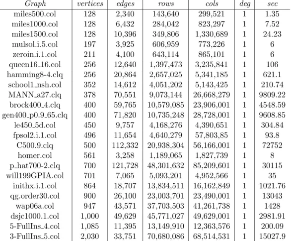
5.2.2 Test Cases . . . 109
5.2.3 Experimental Results overQ . . . 110
5.2.4 Experimental Results overF2 . . . 111
5.2.5 NulLAoverF2 vs. other graph coloring algorithms . . . 115
5.2.6 Hard Instances of 3-colorability . . . 120
5.3 Beyond 3-colorability . . . 126
6 Summary and Future Work 131 6.1 Summary . . . 131
6.2 Future Work . . . 133
List of Figures
2.1 Via Schnyder’s theorem,P(G) has dimension at most three. . . 27
4.1 Tur´an graphT(5,3) . . . 64
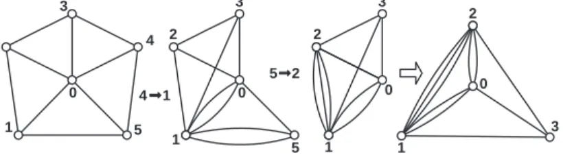
4.2 ConvertingG (the 5-odd-wheel) toH (the 3-odd-wheel) via node merges. . 87
4.3 The odd-wheels are non-3-colorable. . . 89
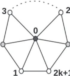
4.4 The (2k+ 1)-odd-wheel to the (2(k+ 1) + 1)-odd-wheel. . . 91
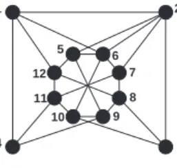
5.1 Koester graph . . . 101
5.2 A graph with a degree four non-3-colorability certificate overF2. . . 103
5.3 Probability tests on cliques and odd-wheels overQ. . . 106
5.4 Probability tests on odd-wheels and cat-ear graphs overF2. . . 128
5.5 Probability tests on Kneser and flower graphs overF2. . . 128
5.6 3,4 and 5 flowers. . . 129
5.7 2,3 and 4 cat-ears. . . 129
5.8 A uniquely 3-colorable graph, the Gr¨otzsch graph, and the Jin graph. . . . 129
5.9 4-critical, near-4-clique-free minimum unsolvable graphs (MUGs). . . 130
5.10 An example of a Liu-Zhang 4-CGU. . . 130
6.1 The line graphs. . . 137
List of Tables
5.1 Experimental investigations of graph 3-colorability overQ. . . 112
5.2 Graphs without 4-cliques overF2. . . 113
5.3 Original graph vs. non-3-colorable subgraph. . . 114
5.4 Graphs with 4-cliques overF2. . . 115
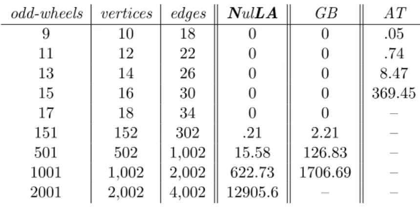
5.5 NulLA, GB and AT on odd-wheel graphs. . . 118
5.6 NulLAvs. Branch-and-Cut andDSATUR. . . 118
5.7 NulLA, GB, AT on graphs with 4-cliques. . . 119
5.8 NulLA, GB, AT on graphs without 4-cliques. . . 119
5.9 Hard instances of graph 3-colorability: MUGs. . . 123
5.10 Hard instances of graph 3-colorability: 4-CGUs. . . 124
5.11 Kn: minimum-degrees for non-(n−1)-colorability certificates. . . 126
6.1 Line graphs: minimum-degrees for non-hamiltonicity . . . 137
Acknowledgments
The process of writing this dissertation was helped along immeasurably by dozens of people who were extremely busy with dozens of projects of their own.
I would like to thank Bernd Sturmfels and Dave Bayer for their support of this project from its earliest stages to the final draft of this dissertation, and I would like to thank Eric Rains for his timely suggestion of exploring encodings over finite fields, which evolved into our most significant computational success.
I would like to thank Chris Hillar for his thoughts and suggestions regarding the Hamiltonian cycle problem, and Alex Woo for his extensive help at the drop of a hat on topics ranging from encodings to Gr¨obner bases to abstract algebra.
I would like to thank my committee members, Zhaojun Bai, Matthew Franklin and Chip Martel, for kindly reading my thesis over the summer break, and for facilitating my unexpected graduation. I would particularly like to thank Dr. Martel for his extensive mentoring throughout my last quarter in regards to the Chancellor’s Teaching Fellowship; co-teaching 122A with him was a pleasure and an inspiration.
I would also like to thank my NulLA collaborators Jon Lee and Peter Malkin. I would like to thank Peter Malkin for the inspiring pictures on his blackboard, for his software engineering expertise, for his unfailing ability to make clean code cleaner and fast code faster, and for his generosity during the last few weeks, when he read and re-read sections of my thesis with inexhaustible patience. I would like to thank Jon Lee for arranging the cluster of 2 GHz machines with 12 MBytes of RAM on behalf of IBM specifically for theNulLAexperiments, for his “hello from [insert exotic location here]” emails which were
always a mixture of quirky humor and 10 papers’ worth of off-hand comments in the form of “you might want to try this...”, for his unfailing latex expertise, and in the end, for his prompt response to my panicked emails begging for last-minute help reading sections of my thesis as my deadlines loomed like a darkening storm... his last comment to me of “write faster!” was the most helpful of all.
And finally, I would like to thank my thesis advisor, Jes´us De Loera, for suggesting the Nullstellensatz Linear Algebra algorithm to me in the very beginning as my dissertation topic; for his patience during my stumbling moments of inarticulate ignorance; for his guidance and insight during critical moments of despair; for his encouragement, optimism and support, and finally for his commitment to academic excellence– without his exacting high standards, this dissertation would be less than half of what it is.
Chapter 1
Introduction
“If I have the belief that I can do it,
I shall surely acquire the capacity to do it even if I may not have it at the beginning.”
–Mohandas Karamchand Gandhi, 1869 - 1948 . “Perplexity is the beginning of knowledge.” –Kahlil Gibran, 1883-1931 .
It is well-known that systems of polynomial equations over an algebraically-closed field can yield compact representations of combinatorial problems. This contrasts with the exponential sizes of systems oflinear inequalities that describe the convex hull of incidence vectors of many combinatorial structures (see [61]).
In [1], N. Alon surveys the use of non-linear polynomials in solving combinatorial problems. Although this technique is not yet as widely used by combinatorists as polyhedral or probabilistic techniques, the literature in this subject continues to expand. Prior work on encoding combinatorial properties includes colorings [2, 38, 19, 24, 41, 43, 44, 49, 39], independent sets [38, 36, 41, 58, 40], matchings [20], and flows [2, 49, 47].
While these polynomial system encodings often suggest an algorithmic approach to solving combinatorial problems (see [1] and therein), they have not yet been widely used for computation. A key issue that we investigate in this dissertation is the use of such polynomial systems to efficiently decide whether a graph, or other combinatorial structure, has a property captured by the polynomial system and its associated ideal. We call this the combinatorial feasibility problem. We are particularly interested in whether this can be accomplished in practice for large combinatorial structures, such as graphs with many vertices.
It is certainly well-known that the combinatorial feasibility problem can be solved using standard tools in computational algebra such as Gr¨obner bases. Nevertheless, it has been experimentally demonstrated that current Gr¨obner bases implementations often cannot directly solve polynomial systems with hundreds of equations. This dissertation proposes the Nullstellensatz Linear Algebra algorithm (NulLA), which instead relies on the experimentally-observed low degrees of Hilbert’s Nullstellensatz forcombinatorial poly-nomial systems, and on large-scale, sparse linear algebra computations.
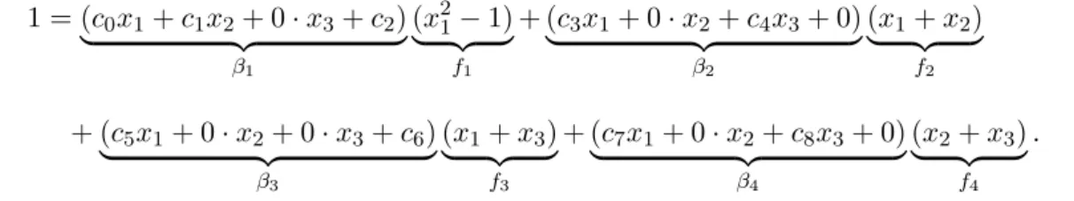
For a hard combinatorial problem (e.g., graph 3-colorability), we associate a sys-tem of polynomial equationsJ ={f1 =· · ·=fs= 0}such that the systemJ has a solution if and only if the combinatorial problem has a feasible solution. Hilbert’s Nullstellen-satz (see e.g.,[13]) states that the system of polynomial equations has no solution over an algebraically-closed field Kif and only if there exist polynomials β1, . . . , βs∈K[x1, . . . , xn] such that 1 =Pβifi. Thus, when the polynomial systemJ has no solution, there exists a
infeasible.
The central idea behind NulLA is to generate a finite sequence of linear alge-bra systems based on Nullstellensatz certificates of increasing degree. These linear algealge-bra systems eventually become feasible if and only if the underlying combinatorial problem is
infeasible. Given a system of polynomial equations, we fix a tentative degree k for the coefficient polynomials βi in the certificates. We decide whether there is a Nullstellensatz certificate with coefficients of degree ≤k by solving a system of linear equations over the fieldKwhose variables are in bijection with the coefficients of the monomials of the polyno-mialsβ1, . . . , βs. If this linear system has a solution, we have found a certificate; otherwise,
we repeat and try a higher degree for the polynomials βi. This process is guaranteed to
terminate because, in order for a Nullstellensatz certificate to exist, the degrees of the poly-nomialsβi cannot be more than known bounds (see [30] and references therein). We explain
the details of NulLAin Chapter 3.
Our method can be seen as a general-field variation of work by Lasserre [33], Laurent [34], Parrilo [53] and many others, who study the problem of minimizing a general polynomial function f(x) over a real algebraic variety with finitely many points. Laurent proved that when the variety consists of the solutions to a zero-dimensional radical ideal I, the optimization problem min{f(x) : x ∈ variety(I)} is equivalent to a finite sequence of semidefinite programs terminating with the optimal solution (see [34]). There are two key observations that speed up practical calculations considerably: (1) when dealing with feasibility, rather than optimization, linear algebra replaces semidefinite programming, and (2) there are methods for controlling the length of the sequence of linear algebra systems,
including finite field computations instead of calculations over the reals, and the reduction of matrix size by symmetries [39]. See Section 5.1 for details.
From commutative algebra, there are well-known upper bounds on the degrees of the coefficients βi in the Hilbert Nullstellensatz certificates for general systems of
polyno-mials, and they turn out to be sharp (see [30]). For instance, the following well-known example (due to Mora, Lazard, Masser, Philippon, and Koll´ar) shows that the degree ofβ1 is at least dm :
f1 =xd1, f2 =x1−xd2, . . . , fm−1=xm−2−xdm−1, fm= 1−xm−1xdm−1 .
But polynomial systems for combinatorial optimization problems are not necessarily patho-logically complicated. In fact, polynomial systems for combinatorial optimization problems are often extremely symmetric with homogeneous polynomials of similar structure, and we now know that the upper bounds on their Nullstellensatz certificates are sometimes much lower. The natural question is: How large are the minimum-degrees of the associated Nullstellensatz certificates of infeasibility?
There is a fascinating connection between Hilbert’s Nullstellensatz and computa-tional complexity. As we will see in Section 4.1, unless P = NP , for every hard combina-torial problem, there must exist an infinite sequence of infeasible instances for which the minimum-degree of a Nullstellensatz certificate, for the associated system of polynomial equations, grows arbitrarily large. This was first observed by L. Lov´asz, who then proposed the problem of explicitly finding graphs exhibiting such growth (see [41]). A main contri-bution of this dissertation is to explicitly describe the growth in degree of specific families of graphs. In particular, we establish the following main theorem (Section 4.2):
Given a graph G, let α(G) denote the size of the largest independent set in G. A minimum-degree Nullstellensatz certificate (associated with the Lov´asz encoding of Lemma 2.1.1) for the non-existence of an independent set of size greater thanα(G) has degree equal toα(G) and contains at least one monomial per independent set in G.
This dissertation is organized as follows. In Chapter 2, we describe various en-codings for an assortment of NP-complete and combinatorial decision problems. We survey existing encodings for independent set, graphk-colorability and SAT, and present new en-codings for Hamiltonian cycle, graph k-colorability, max cut, edge chromatic number and graph planarity. In Chapter 3, we describe the Nullstellensatz Linear Algebra (NulLA) algorithm. In Chapter 4, we explore the relationship between Nullstellensatz certificates and complexity theory, touching P vs. NP, NP vs. coNP and NP as a proper or improper subset of EXPTIME. We also prove a range of theoretical results concerning growth in the minimum-degree of both non-k-colorability, and non-existence of an independent set of size k, Nullstellensatz certificates. In Chapter 5, we present our experimental results, and a variety of mathematical techniques for optimizing NulLA, and in Chapter 6, we presents our conclusions and suggestions for future directions of research.
Chapter 2
Encodings
“The formulation of a problem is often more essential than its solution, which may be merely a matter of mathematical or experimental skill.” –Albert Einstein, 1879–1955 . In this chapter, we demonstrate the ease and simplicity of encoding combinatorial problems as systems of polynomial equations. Our constant goal throughout this chapter is computation with algebraic methods; towards that end, we will often present more than one encoding for the same combinatorial problem. The purpose of these multiple encodings is not only to demonstrate a variety of encoding techniques, but also to eventually compare and contrast encodings from a computational perspective (see Chapter 5).
By encoding, we simply mean the following: given an instance of a “yes/no” de-cision question, we can convert it in polynomial-time (in the input size of the instance) to a system of polynomial equations such that the system has a solution if and only if the underlying instance has a “yes” answer. It is important to emphasize the polynomial-time nature of these conversions; otherwise, we could simply solve the “yes/no” decision
ques-tion beforehand and represent every “yes” instance as the equaques-tion “1=1”, and every “no” instance as “1=0”. This definition is formalized as follows:
Definition 2.0.1 Given a language L, if there exists a polynomial-time algorithm A that takes as input a stringI, and produces as output a system of polynomial equations such that the system has a solution if and only if I ∈L, then we say that the system of polynomial equations encodes I.
We use the formal terminology of languages (see [59] for relevant background), instead of the more familiar vocabulary ofyes/no decision problems to bypass any technical difficulties with the “encodings” of the instances themselves (such as adjacency lists vs. adjacency matrices of graphs). However, since yes/no decision questions are equivalent to languages, we will often use these terms interchangeably, especially when referring to NP-complete problems. We also note that, because Definition 2.0.1 stipulates that the algorithm Aconstructing the system of equations runs inpolynomialtime, this means that the system of equations can be written down in polynomial space. Intuitively, when converting a problem from the representation stipulated by the language (such as the adjacency matrix or adjacency list of a graph) to a system of polynomial equations, we must avoid introducing an exponential number of variables or equations, or introducing degrees or coefficients are exponentially long in terms of bit-length. However, given a polynomialg(n) where nis the input size of the instance, by stipulating that the encoding can be constructed inO(g(n)) time, we can be certain of the following bounds: given a system of polynomial equations f1 = · · · = fs = 0 that encodes an instance I, the number of equations is O(g(n)), the
maximum number of monomials in anyfi isO(g(n)), and bit-size of the largest coefficient
in any fi is O(g(n)). This idea is formalized in the following definition, which we use
extensively in Section 4.1:
Definition 2.0.2 Given a languageLand a polynomialg(n), if the algorithmAfor encod-ing a strencod-ingI of lengthnruns inO(g(n))time, then we say thatLhas an O(g(n))-encoding.
In this chapter, we present encodings for independent set (Section 2.1), graph k -colorability (Section 2.2), Hamiltonian cycle (Section 2.3), graph planarity (Section 2.4), edge-chromatic number (Section 2.5), max-cut (Section 2.6), and finally, SAT (Section 2.7). We note that by displaying an encoding for SAT, we can easily construct encodings forall NP-complete problems via polynomial reductions to SAT. However, this approach is not computationally practical because of the increase in the number of variables/equations in the systems. Furthermore, we will see later that encodings using constraints of the form xi(xi−1) seem to behave badly with algebraic methods such as NulLA(see Section 4.2),
but other type of constraints (e.g. root of unity constraints such as in graph 3-colorability) do behave better in practice (see Chapter 5).
Although the encodings presented in this chapter are not always very interesting in and of themselves, we explore their value in terms of providing insight into the underlying problem (Section 5.2.6), or in terms proving bounds on their associated identities (Section 4.2), or most importantly, in terms of being able to compute effectively on large combina-torial structures, such as graphs. The foremost question for us is the following: how can we best capture the combinatorial structure of an NP-complete problem with respect to Hilbert’s Nullstellensatz?
Before we begin, we clarify our terms and notation: Adj(i) denotes the set of nodes adjacent to node i; a zero-dimensional system of equations is a system of equations with a finite number of solutions; every encoding presented is overC(the complex numbers) unless otherwise specified, and all graphs are assumed to be simple. For all other concepts and basic definitions from graph theory, we refer to [16].
2.1
Independent Set
Given a graph G, astable setor independent setinG is a subset of vertices such that no two vertices in the subset are adjacent. The size of the largest independent set inG is called thestability number, orindependence number, of G, and is denoted byα(G). The decision question of determining whether a given graph has an independent set of sizek is NP-complete [21], and can be encoded as the following system of polynomial equations: Lemma 2.1.1 (L. Lov´asz [41]) A graph G has an independent set of size k if and only if the following zero-dimensional system of equations
x2i −xi= 0 , for every node i∈V(G) ,
xixj = 0 , for every edge{i, j} ∈E(G) , n
X
i=1
xi−k= 0 ,
has a solution. Moreover, the number of solutions equals the number of distinct independent sets of size k.
Proof: If the graph G has an independent set I of size k, we simply assign the variables associated with vertices in I to have value one, and all other variables to have value zero.
Then, the above system of equations is satisfied. If the above system of equations is satisfied, the equationsx2
i−xi= 0 force every variable to take on 0/1 values. The equationsxixk = 0
show that no two vertices assigned the value one are adjacent. The last equation shows that exactlykvariables have the value one: thus, those variables correspond directly to vertices in an independent set of size k.
We now show that the number of solutions equals the number of distinct indepen-dent sets of sizek. We have previously shown that independent sets correspond to solutions and solutions correspond to independent sets, but we now show that the map between the two sets is bijective. Given any independent set of size k, we simply assign every variable in the independent set to be one and all other variables to be zero. Thus, given two inde-pendent sets, I1 and I2, if they map to the same solution (the same 0/1 vector), then the same vertices must have been present in both sets andI1 =I2. Thus, the map is injective, or one-to-one. Since we have already shown that every solution maps to an independent set (the map is surjective or onto), we have shown that the map is bijective and the number of solutions is equal to the number of distinct independent sets of sizek. 2
In Section 4.2, we explicitly describe the Nullstellensatz certificates associated with this system of polynomial equations.
2.2
Graph
k
-Colorability
The problem of graph k-colorability is as follows: given a graphGand an integer k, can Gbe colored with kcolors such that no two adjacent vertices have the same color?
This problem is known to be NP-complete [21]. In addition to being hard, it is also an interesting practical problem, having applications to fields as varying as compiler optimiza-tion and scheduling. In this secoptimiza-tion, we present several encodings for graph k-colorability: a degree-k encoding over C, a degree-2 encoding over C, and our most computationally successful encoding, a degree k-encoding over Fp (the algebraic closure of the finite field
withp elements).
We extensively studied the encodings described in this section, both from the theoretical perspective (Section 4.3), and from the computational perspective (Chapter 5). We begin with the following remark:
Lemma 2.2.1 Given a graphG withn vertices, let I be the ideal
I = * xk1−1, . . . , xkn−1, k−1 X d=0 xki−1−dxdj | {z } {i,j}∈E(G) + .
Then I is a radical ideal. Moreover,dim(C[x1, . . . , xn]/I) is equal to the number of points
in variety(I).
Proof: Recall that a “square-free” polynomial is a polynomial with no repeated factors (e.g., (x+ 3)2(x+ 6) is not square-free, whereas (x+ 3)(x+ 6) is square-free). For every xi, the ideal I contains the square-free, univariate polynomial x3i −1. Thus, I is a radical
ideal by [12], pg. 39-41, Proposition 2.7. Therefore, by [13], pg. 232, Proposition 8 (ii), dim à C[x1, . . . , xn] I ! =|V(I)|. 2
We will see later that |V(I)| is equal to the number of k-colorings of a graph multiplied byk!. Therefore, Lemma 2.2.1 allows us to compute the number ofk-colorings of a graph by computing the dimension (as a vector space) of the quotient ringC[x1, . . . , xn]/I. Our first encoding, degree-k over C, is a generalization of an encoding proposed by Bayer for the case of 3-colorability.
Lemma 2.2.2 (Bayer [5]) A graph G is k-colorable if and only if the following zero-dimensional system of equations
xki −1 = 0 , for every node i∈V(G) ,
k−1
X
d=0
xki−1−dxdj = 0 , for every edge{i, j} ∈E(G) ,
has a solution. Moreover, the number of solutions equals the number of distinctk-colorings multiplied by k!.
Proof: Assume thatGisk-colorable, and assign the colors to thekroots of unity. Clearly, the vertex equations (xk
i −1 = 0) are satisfied. Since the graph is k-colorable, there exists
a coloring such that no two adjacent vertices have the same color. Therefore, given an edge
{i, j} ∈E(G), the root of unity assigned to xi does not equal the root of unity assigned to
xj, and we see that
xk i −xkj xi−xj = k−1 X d=0 xki−1−dxdj =⇒ xki −xkj = (xi−xj) k−1 X d=0 xki−1−dxdj = 0 .
Since xi 6= xj, the factor xi−xj 6= 0. Thus,
Pk−1
d=0xki−1−dxdj = 0, and the edge equations
are satisfied.
Conversely, assume there exists a solution to the above system of equations. The vertex equations (xk
roots of unity. We will now show that no two adjacent vertices are assigned the same color. To prove this, assume the contrary: assume that for some edge {i, j}, xi and xj are both
assigned the same root of unity,β. Then,
0 =
k−1
X
d=0
xki−1−dxdj =kβk−16= 0
Thus, every adjacent pair of vertices is assigned a different color.
We now show that the number of solutions equals number of distinct k-colorings multiplied by k!. We have previously shown that k-colorings correspond to solutions and solutions correspond to k-colorings, but we now show that the map between the two sets is bijective. We first explicitly map the k colors to the k roots of unity. For example, in the case of k = 3, we assign red → e2πi/3, green → e4πi/3, and blue → e2πi = 1. Under this map, if two colorings of the graph,C1 andC2, map to the same solution, then the two colorings are the same. Thus, the map is injective, or one-to-one. Since we have already shown that every solution maps to a coloring (the map is surjective or onto), we have shown that the map is bijective. Since there are k! ways to assignkcolors to thek roots of unity, the number of solutions is equal to the number of distinctk-colorings multiplied byk!. 2
The following corollary concerning k-colorable subgraphs easily follows from this result.
Corollary 2.2.3 A graph G has a k-colorable subgraph with R edges if and only if the following zero-dimensional system of equations has a solution:
X
{i,j}∈E(G)
For every vertex i∈V(G):
xki −1 = 0 .
For every edge {i, j} ∈E(G):
y2ij−yij = 0, yij¡xki−1+xki−2xj+· · ·+xkj−1¢= 0 .
Proof: For a k-colorable subgraphH with R edges, we set yij = 1 if edge {i, j} ∈E(H)
or 0 otherwise. By Lemma 2.2.2, the resulting subsystem of equations has a solution. Con-versely, from a solution, the subgraph H in question is described by yij = 1. By Lemma
2.2.2 above, a solution maps to ak-coloring. 2
We now present a new degree two encoding of graph k-colorability, based on the idea of “partitioning” the graph intok disjoint sets. Thus, every vertex appears in exactly one partition, and the order of the partitions defines the order of the cycle.
Lemma 2.2.4 Let C[xip], where 1≤i≤n and 1≤p≤k, be a polynomial ring. A graph
G is k-colorable if and only if the following zero-dimensional system of equations has a solution.
For every node i∈V(G):
k X p=1 xip −1 = 0 ,
For every edge {i, j} ∈E(G) andp= 1, . . . , k:
For every node i∈V(G) and p= 1, . . . , k:
xip(xip−1) = 0.
Proof: If the graph Gis k-colorable, then assignxir to be 1 if vertexihas the r-th color, and all other xip to be 0. Clearly, the first and third equations are satisfied. Furthermore,
since no two adjacent vertices have the same color, no two adjacent vertices are in the same partition; thus, the second equation is satisfied.
Conversely, assume that there exists a solution to the above system of equations. By the first and third equations, clearly every vertex appears in only one partition. Fur-thermore, by the second equation, no two adjacent vertices are in the same partition. Thus,
the vertex/partition mapping corresponds to ak-coloring. 2
Finally, we come to our most computationally successful encoding: graph k -coloring over Fp, where k and p are relatively prime. Before we describe this encoding,
we introduce a few well-known facts from algebra.
Lemma 2.2.5 The equation xn−1 = 0 has n distinct roots over Fp, when p is relatively
prime to n.
Proof: Thediscriminant of a polynomial f(x) =anxn+a
n−1xn−1+· · ·+a0 is defined to be
disc(f) = (−1)n(n−1)/2
an Res(f, f
0)
When the discriminant is non-zero, f does not have multiple roots. In this case, f(x) = xn −1, and f0(x) = nxn−1. The resultant is the determinant of the Sylvester matrix,
displayed below: Syl(f, f0) = ¯ ¯ ¯ ¯ ¯ ¯ ¯ ¯ ¯ ¯ ¯ ¯ ¯ ¯ ¯ ¯ ¯ ¯ ¯ ¯ ¯ ¯ ¯ ¯ ¯ ¯ ¯ ¯ ¯ ¯ ¯ ¯ ¯ ¯ ¯ ¯ ¯ ¯ ¯ ¯ ¯ 1 0 · · · · · · 0 −1 0 · · · · · · 0 0 1 0 · · · · · · 0 −1 0 · · · 0 .. . . .. ... . .. ... ... .. . . .. ... . .. ... 0 0 · · · · · · 0 1 0 · · · · · · 0 −1 n 0 · · · · · · · · · · · · · · · · · · · · · 0 0 n 0 · · · · · · · · · · · · · · · · · · 0 .. . . .. ... ... ... ... ... ... ... .. . . .. ... ... ... ... ... ... 0 0 · · · · · · 0 n 0 · · · · · · · · · 0 ¯ ¯ ¯ ¯ ¯ ¯ ¯ ¯ ¯ ¯ ¯ ¯ ¯ ¯ ¯ ¯ ¯ ¯ ¯ ¯ ¯ ¯ ¯ ¯ ¯ ¯ ¯ ¯ ¯ ¯ ¯ ¯ ¯ ¯ ¯ ¯ ¯ ¯ ¯ ¯ ¯ n−1 rows nrows
Thus, the discriminant is±nn mod p. This is easy to see by expanding around the last n
rows of the Sylvester matrix when taking the determinant. Since gcd(n, p) = 1, ±nn 6≡ 0 mod p, and because the discriminant is non-zero, the roots of the equationxn−1 = 0 are
distinct. 2
Lemma 2.2.6 A graphGisk-colorable if and only if the following zero-dimensional system of equations
xki −1 = 0 , for every node i∈V(G) ,
k−1
X
d=0
xki−1−dxdj = 0 , for every edge{i, j} ∈E(G) ,
has a solution overFp, wherekandpare relatively prime. Moreover, the number of solutions equals the number of distinctk-colorings multiplied by k!.
Proof: This proof follows from Lemmas 2.2.2 and 2.2.5. Since thek distinct roots of unity (in this case, ω, ω2, . . . , ωk−1,1) can be mapped to the k distinct colors, we see again that the number of solutions equals the number of distinctk-colorings multiplied byk!. 2
We conclude with an observation that foreshadows a result from our experimental investigations: although the colorings of a given graph are completely described by a system of polynomial equations such as Lemma 2.2.6, it may sometimes be computationally useful to addextraequations to these systems (see Chapter 5, Section 5.1.2). These extra equations should capture extra combinatorial properties of the underlying graph, which allow us to simplify our computations. For example, when testing for 3-colorability, it is logical to search the graph for triangles as a means of reducing computation time. In our case, a triangle formed by the vertices {i, j, k} forces the variables xi, xj, xk to take on different
colors/roots of unity. In order to formalize the idea of a triangle equation, we need the following well-known fact from algebra:
Proposition 2.2.7 ([17]) IfG is a finite group such that, for all positive integersn divid-ing its order, Gcontains at most nelements x satisfying xn−1 = 0, then G is cyclic.
Therefore, the group formed by the roots of unity ofxk−1 = 0 is cyclic, regardless
of whether the field is C or Fp. The roots of unity overC are generated by powers of the
primitive root e2πi/k, while the roots of unity over F
p can be described as powers of a
primitive rootω:
ω, ω2, . . . , ωk−1,1
Lemma 2.2.8 Given a graph G and an integer k, encoded as the system of polynomial equations from Lemma 2.2.2 or 2.2.6, if G contains a k-clique {xi1, xi2, . . . , xik} as a
sub-graph and d is any integer such thatd6 |k, then the following equation
xdi1+xdi2 +· · ·+xdik = 0 (2.1)
can be added to the system of equations without changing the set of solutions.
Proof: If the system of equations from Lemma 2.2.2 or 2.2.6 has a solution, we must show that any such solution also satisfies Eq. 2.1. The following proof applies to the system of equations from either lemma. When the system of equations (either system) has a solution, no two adjacent vertices are assigned the same color. In particular, the vertices
{i1, i2, . . . , ik}corresponding to the k-clique are each assigned a different color. Therefore,
the corresponding variables xi1, xi2, . . . , xik represent the complete set of the k roots of unity. If the variablesxi1, xi2, . . . , xik areeach raised to thedpower, the values of the roots
are simply permuted (sincedis not a factor ofk); therefore,xdi1, xdi2, . . . , xdik also represents the complete set of the kroots of unity. Furthermore, recall
xk−1 = (x−1)(xk−1+xk−2+· · ·+x+ 1) = 0.
Therefore, any primitive root satisfies (xk−1+xk−2+· · ·+x+ 1) = 0, and the sum of the complete set of thekroots of unity is zero. Thus, if the system of equations has a solution, then the system of equations,along with Eq. 2.1, also has a solution. 2
In Chapter 5, Section 5.1.2, we will see the computational advantage of including these types of subgraph equations, and the advantage of having flexibility in choosing the degreed.
2.3
Hamiltonian Cycle
A Hamiltonian cycle is a cycle that passes through every vertex exactly once. Given a graph Gand an integerk, it is NP-complete to determine ifGhas a Hamiltonian cycle, or if G has a cycle of length k [21]. In this section, we describe an encoding for finding a cycle of length k in a graph, and then as a corollary, describe an encoding for Hamiltonian cycle. We also describe a graph-theoretic application that arises naturally from these encodings. We conclude by presenting an encoding of Hamiltonian cycle over
Fp, and also demonstrating a degree two encoding similar to the encoding presented for
graphk-colorability.
Lemma 2.3.1 A simple graph G has a cycle of length L if and only if the following zero-dimensional system of polynomial equations has a solution:
à n X i=1 yi ! −L= 0 . (2.2)
For every node i= 1, . . . , n:
yi(yi−1) = 0, n Y s=1 (xi−s) = 0 , (2.3) yi Y j∈Adj(i) (xi−yjxj+yj)(xi−yjxj−yj(L−1)) = 0 . (2.4)
Proof: Suppose that a cycle C of length L exists in the graph G. We set yi = 1 or 0
depending on whether or not nodei is in C. Next, starting the numbering at any node of C, we set xi =j if nodei is thej-th node of C. It is easy to check that Eqs. 2.2 and 2.3 are satisfied. Note that if vertexiis not in C,xi can be set to any value between 1 and n.
To verify Eq. 2.4, note that because C has length L, if vertex i is thej-th node of the cycle, then one of its neighbors, sayk, must be the “follower”, namely the (j+ 1)-th element of the cycle. If j < L, then the factor (xi−xk+ 1) = (xi−(xk−1)) = 0 appears in the product equation associated with the i-th vertex, and the product is zero. Ifj =L, then the factor (xi−xk−(L−1)) = 0 appears, and the product is again 0. For all other
vertices xi not in C, simply set xi to any value between 1 and n(satisfying Eq. 2.3), and then “turn them off” by setting yi = 0, which causes Eq. 2.4 to be automatically satisfied.
Thus, every equation in the polynomial system is satisfied.
Conversely, from a solution of the system above, we see that L variables yi are
“turned on”; let these variable be the setC. Furthermore, we see that every variable takes on a value between 1 andn. We claim that the nodes i∈C form a cycle. Because yi 6= 0,
the polynomial of Eq. 2.4 must vanish. Thus, for everyj∈C,
either (xi−xj+ 1) = 0, or (xi−xj−(L−1)) = 0.
Note that Eq. 2.4 reduces to this form when yi and a particularyj equal one. Therefore, either vertex iis adjacent to a vertex j (with yj = 1) such that xj equals the next integer
value (xi + 1 = xj), or xj = xi −L+ 1. Consider the variable xi1 which takes on the
smallest value of any variable in C. For xi1, Eq. 2.4 cannot cancel by being adjacent to a variable xj = xi1 −L+ 1 (because then xi1 would not be the smallest value in C).
Thus, for variable xi1, Eq. 2.4 must cancel because it is adjacent to a variable xi2 which
takes on the next highest value. This condition holds for the next L−2 variables in C: Eq. 2.4 cancels because each variable is adjacent to a variable taking on the next high-est value. Thus, the variables in C traverse a consecutive sequence of integers from xi1
to xiL. Therefore, xiL must take on the largest value of any variable in the set C: thus,
it must be adjacent to a variable taking on the value xj = xiL+L−1. The only point
inCsatisfying that criteria isxi1. Thus, the points inCdescribe a cycle of lengthLinG. 2
We have the following corollary.
Corollary 2.3.2 A graph G has a Hamiltonian cycle if and only if the following zero-dimensional system of equations has a solution. For every node i ∈ V(G), we have two equations: n Y s=1 (xi−s) = 0 , and Y j∈Adj(i) (xi−xj+ 1)(xi−xj−(n−1)) = 0 .
The number of Hamiltonian cycles in the graph equals the number of solutions of the system divided by 2n.
Proof: Clearly whenL=nwe can just fix allyi to 1, thus many of the equations simplify
or become obsolete. We only have to check the last statement on the number of Hamiltonian cycles. For that, we remark that no solution appears with multiplicity because the ideal is radical. That the ideal is radical is implied by the fact that every variable appears as the only variable in a unique square-free polynomial (see page 246 of [31]). Finally, note for every cycle there are n ways to choose the initial node to be labeled as 1, and then two
possible directions to continue the labeling. 2
These results also apply to directed graphs; thus, we can also consider paths or cycles with orientation. We can also use the polynomials systems above to investigate the
distribution of cycle lengths in a graph (similarly for path lengths and cut sizes). This topic has several outstanding questions. For example, a still unresolved question of Erd¨os and Gy´arf´as [57] asks: If G is a graph with minimum-degree three, is it true that G always has a cycle having length that is a power of two? We define the cycle-length polynomial
as the square-free univariate polynomial whose roots are the possible cycle lengths of a graph (same can be done for cuts). Considering Las a variable, the reduced lexicographic Gr¨obner basis (withL the last variable) computation provides us with a unique univariate polynomial onL that is divisible by the cycle-length polynomial of G.
Before we display our encoding over Fp, where p and n are relatively prime, we
recall that there exists a primitive root of unity forxn−1 = 0, via Proposition 2.2.7 from
Section 2.2.
Lemma 2.3.3 Let G be a connected graph with n vertices. Then G has a Hamiltonian cycle if and only if the following zero-dimensional system of equations
xn
i + 1 = 0 , for every node i∈V(G) ,
Q
j∈Adj(i)(ωxi+xj) = 0 , for every node i∈V(G) ,
has a solution overFp, where p and n are relatively prime, and ω is an n-th primitive root
of unity.
Proof: Suppose there exists a Hamiltonian cycle in the graphG. We can begin the num-bering at an arbitrary vertex, and assign the vertices to be powers ofω; thus, a Hamiltonian cyclevi1, vi2, . . . , vin impliesxi1 =ω, xi2 =ω2, and xin =ωn= 1. Clearly, the vertex
equa-tionsxn
is adjacent to the next highest power of ω in the cycle. Thus,ωxi1 −xi2 =ω·ω−ω2 = 0.
Therefore, every edge equation is satisfied.
Conversely, from a solution to the system above, we see that every variable is assigned a root of unity. Consider thelowest power of ω assigned to any variable. Because the edge equations are satisfied, every variable must be adjacent to a variable taking on the value of thenext highest power of ω. Since there are nvariables, we must eventually come to a variable assigned the value ωn = 1. That variable must be adjacent to the variable
taking on the value ω; thus, the lowest power ofω assigned to any variable is one, and the
order of the powers ofω define a Hamiltonian cycle inG. 2
We observe that this encoding, as is, does not necessarily lend itself to computation. In order to compute with this encoding, we would have to treat ω as an extra value in our field, and compute over the splitting fieldFp∪ω. This encoding is also easily transferable to
an encoding over C; however, the computational difficulty of computing over the splitting fieldQ∪ω is similar. However, byadding a few equations to the encoding,ωcan be treated as a variable and not as a fixed primitiven-th root of unity. For example, if the equation ωn−1 = 0, and the set of equations
yk(ωk−1) = 0,
wherekis any factor dividingn, are added to the encoding of Lemma 2.3.3, thenωis simply a variable which can only take on the value of a primitive n-th root of unity, even if n is not a prime number. Another set of equations which ensuresω is a variable only taking on
the value of a primitive n-th root of unity is the following:
ωk(n−1)+ωk(n−2)+· · ·+ωk+ 1, for 1≤k≤n .
We can also use the cyclotomic polynomial [17], denoted by Φ(n), which is the polynomial whose roots are the primitive n-th roots of unity. For example, the first ten cyclotomic polynomials are as follows:
Φ1(x) =ω−1 , Φ6(x) =ω2−ω+ 1,
Φ2(x) =ω+ 1, Φ7(x) =ω6+ω5+ω4+ω3+ω2+ω+ 1, Φ3(x) =ω2+ω+ 1, Φ8(x) =ω4+ 1,
Φ4(x) =ω2+ 1, Φ9(x) =ω6+ω3+ 1,
Φ5(x) =ω4+ω3+ω2+ω+ 1, Φ10(x) =ω4−ω3+ω2−ω+ 1. (2.5)
We conclude by presenting a degree two encoding of Hamiltonian cycle. This encoding is similar to the one presented for graphk-colorability, and is again based on the idea of “partitioning” the graph intondisjoint sets. Thus, every vertex appears in exactly one partition, and the order of the partitions defines the order of the cycle.
Lemma 2.3.4 Let C[xip], where1≤i, p≤n, be a polynomial ring. Given a simple graph
G, thenG has a Hamiltonian cycle if and only if the following zero-dimensional system of equations has a solution.
For every node i∈V(G):
Xn p=1 xip −1 = 0 , and X j∈Adj(i) xinxj1+nX−1 p=1 xipxj(p+1) −1 = 0 .
For every node i∈V(G) and p= 1, . . . , n:
xip(xip−1) = 0.
Proof: If the graph G has a Hamiltonian cycle, then start the labeling at an arbitrary vertex in the cycle, and assign xir to be 1 if vertex iis the r-th vertex on the cycle, and all other xip to be 0. Clearly, the first and third equations are satisfied. The second equation
is satisfied since every vertexiis adjacent to a vertex j which is placed in thenext highest partition, or vertex i is the n-th vertex on the cycle, in which case it is adjacent to the vertex placed in the first partition.
Conversely, assume that there exists a solution to the above system of equations. By the first and third equations, clearly every vertex appears in only one partition. Con-sider a vertexiin thelowest possible partition. That vertex cannot be in then-th partition, because, in that case, the second equation is only satisfied if it is adjacent to a vertexj in the first partition (thus, contradicting the minimality of the partition ofi). Thus, vertexi must be adjacent to a vertex j in thenext highest partition. This condition holds for then vertices in the graph. Finally, since the vertex in the n-th partition cannot be adjacent a vertex in a higher partition, it must be adjacent to a vertex in the first partition. Thus, the vertex in the lowest possible partition must be in the first partition, and the vertex/partition
order defines a Hamiltonian cycle in the graph. 2
We conclude by noting that the encodings presented in this section are notO(g(n ))-encodings for any polynomial g(n). For example, in Lemma 2.3.1, for any vertex i the equation Qns=1(xi −s) = 0 has 2n terms when expanded. Lemma 2.3.3 is also not an
O(g(n))-encoding for any polynomialg(n), because, given a graph containing a vertexiwith degree n−1, the equation Qj∈Adj(i)(ωxi−xj) has 2n−1 terms when expanded. However,
it may yet be possible to compute using these encodings because the polynomials can be represented concisely as the product of linear factors. Algebraic methods exploiting these linear factors have yet to be developed or investigated. Despite these problems with the encoding size, we recall that the Hamiltonian cycle problem remains NP-complete even for k-regular graphs with k ≥ 3 [54]. In this case, when restricted to k-regular graphs for a fixed k, Lemma 2.3.3 is anO(n)-encoding where nis the number of vertices in the graph.
2.4
Graph Planarity
Aplanar graph is any graph that can be embedded (or drawn) in the plane in such a way that no two edges cross (see [16] for details). Although graph planarity is solvable in polynomial-time, we present an encoding as a system of polynomial equations for two reasons: 1) we are interested in whether or not this system of polynomial equations is likewise solvable in polynomial time, and 2) can the techniques displayed in this encoding be used for other combinatorial problems. The encoding we present here for testing graph planarity is based on Schnyder’s characterization of planarity in terms of the dimension of a partially-ordered set or poset [55]: For an n-element poset P, a linear extension is an order-preserving bijection σ :P → {1,2, . . . , n}. The poset dimension of P is the smallest integertfor which there exists a family oftlinear extensionsσ1, . . . , σtofP such thatx < y
in P if and only if σi(x)< σi(y) for allσi. Theincidence poset P(G) of a graphG(V, E) is the partially-ordered set of height two on the union of nodes and edges, where we sayx < y
ifx is a node andy is an edge, and y is incident to x.
Example 2.4.1 (Posets and Planar Graphs) LetGbe the planar square graph. Here we display the incidence posetP(G) and its three corresponding linear extensions.
1 2 3 4 (1,2) (2,3) (3,4) (4,1) (1,2) (2,3) (3,4) (4,1) 3 4 2 1 3 4 1 2 (4,1)3 (3,4) (2,3) 2 (1,2) 1 4 (2,3) (3,4) (1,2) (4,1) 1 2 4 3 G = square P(G) linear extensions
Figure 2.1: Via Schnyder’s theorem, P(G) has dimension at most three.
Lemma 2.4.2 (Schnyder’s theorem [55]) A graph G is planar if and only if the poset dimension of P(G) is no more than three.
We begin by encoding the decision question of poset dimension as a system of polynomial equations.
Lemma 2.4.3 Let P = (E, >) be a poset, and C[x{i}k,∆{ij}k, sk] be a polynomial ring in
p|E|+(|E|2−|E|)+pvariables (wherei= 1, . . . ,|E|,j = 1, . . . ,|E|,j 6=i, andk= 1, . . . , p).
Then P has poset dimension at most p if and only if the following system of equations has a solution:
For k= 1, . . . , p:
|E|
Y
s=1
(x{i}k−s) = 0 , for every i∈ {1, . . . ,|E|}, and
sk Y 1≤i<j≤|E| x{i}k−x{j}k −1 = 0 . (2.6)
For k= 1, . . . , p, and every ordered pair of comparable elements ei > ej in P :
x{i}k−x{j}k−∆{ij}k= 0 . (2.7)
For every ordered pair of incomparable elements of P (i.e., ei 6> ej and ej 6> ei) : p Y k=1 ¡ x{i}k−x{j}k−∆{ij}k¢= 0 , p Y k=1 ¡ x{j}k−x{i}k−∆{ji}k¢= 0 . (2.8)
For k= 1, . . . , p, and for every pair {i, j} ∈ {1, . . . ,|E|}: |EY|−1 d=1 (∆{ij}k−d) = 0 , |EY|−1 d=1 (∆{ji}k−d) = 0 .
Proof: With Eqs. 2.6 and 2.7, we assign distinct numbers 1 through |E| to the poset elements, such that the properties of a linear extension are satisfied. Eqs. 2.6 and 2.7 are repeated p times, so p linear extensions are created. If the intersection of these extensions is indeed equal to the original poset P, then for every incomparable pair of elements in P, at least one of the p linear extensions must detect the incomparability. But this is in-deed the case for Eq. 2.8, which says that for thel-th linear extension, the values assigned to the incomparable pairei, ejdo not satisfyx{i}l< x{j}l, but instead satisfyx{j}l> x{i}l. 2
We will now use the encoding of poset dimension as a system of polynomial equa-tions to capture Schnyder’s criterion for graph planarity.
Lemma 2.4.4 Given a simple graphG(V, E) withn vertices and m edges, let C[zij, x{i}k,
y{ij}k,∆{ij,i},k,∆{ij,uv},k, sk]be a polynomial ring in
¡
m+ 3(2m+m(m−1) +m+n+ 1)¢
variables (where 1 ≤ i ≤ n,{i, j} ∈ E(G),{u, v} ∈ E(G), and 1 ≤ k ≤ 3). Then G has a planar subgraph with K edges if and only if the following zero-dimensional system of equations has a solution:
For every edge {i, j} ∈E(G):
zij2 −zij = 0,
X
{i,j}∈E(G)
zij −K = 0 .
For k= 1,2,3 , every nodei∈V(G) and every edge {i, j} ∈E(G):
nY+m s=1 (x{i}k−s) = 0, nY+m s=1 (y{ij}k−s) = 0 , sk Y i,j∈V(G) i<j ¡ x{i}k−x{j}k¢ Y i∈V(G), {u,v}∈E(G) ¡ x{i}k−y{uv}k¢ Y {i,j},{u,v}∈E(G) ¡ y{ij}k−y{uv}k¢ = 1 .
For k= 1,2,3, and for every pair of i∈V(G) and incident edge {i, j} ∈E(G):
zij
¡
y{ij}k−x{i}k−∆{ij,i}k¢= 0 .
For every pair of node i∈V(G)and edge{u, v} ∈E(G) that is notincident oni:
zuv
¡
y{uv}1−x{i}1−∆{uv,i}1¢¡y{uv}2−x{i}2−∆{uv,i}2¢¡y{uv}3−x{i}3−∆{uv,i}3¢= 0 ,
zuv
¡
x{i}1−y{uv}1−∆{i,uv}1¢¡x{i}2−y{uv}2−∆{i,uv}2¢¡x{i}3−y{uv}3−∆{i,uv}3¢= 0 .
For every pair of edges {i, j},{u, v} ∈ E(G) (regardless of whether or not they share an endpoint):
zijzuv
¡
zijzuv
¡
y{uv}1−y{ij}1−∆{uv,ij}1¢¡y{uv}2−y{ij}2−∆{uv,ij}2¢¡y{uv}3−y{ij}3−∆{uv,ij}3¢= 0.
For every pair of nodesi, j∈V(G)(regardless of whether or not they are adjacent):
¡
x{i}1−x{j}1−∆{i,j}1¢¡x{i}2−x{j}2−∆{i,j}2¢¡x{i}3−x{j}3−∆{i,j}3¢= 0 ,
¡
x{j}1−x{i}1−∆{j,i}1¢¡x{j}2−x{i}2−∆{j,i}2¢¡x{j}3−x{i}3−∆{j,i}3¢= 0 .
For every ∆index (e.g., ∆{ij,uv}k,∆{ij,i}k , etc.) variable appearing in the above
system:
n+Ym−1
d=1
¡
∆index−d¢= 0 .
Proof: We simply apply Lemma 2.4.3 to the particular pairs of order relations of the incidence poset of the graph. Note that in the formulation, we have added variableszij that
have the effect of “turning on or off” an edge of the input graph. 2
2.5
Edge-Chromatic Number
Theedge-chromatic number of a graph, denoted byχ0(G), is the minimum number
of colors necessary to color every edge such that no two edges incident on the same vertex are the same color. It is easy to see that the edge-chromatic number is bounded from below by ∆(G), the largest vertex degree in the graph. Also, by Vizing’s theorem [16], we know that any graph can be edge-colored with ∆(G) + 1 colors, and therefore, we see
Thus, the question of determining edge-chromatic simplifies to determining whetherχ0(G)
is ∆(G) or ∆(G) + 1. This problem is NP-complete [25], and we encode it as the following system of polynomial equations.
Lemma 2.5.1 Let G be a simple graph with maximum vertex degree ∆. The graph G has edge-chromatic number∆if and only if the following zero-dimensional system of polynomials has a solution:
For every edge {i, j} ∈E(G):
x∆ij −1 = 0 . (2.9)
For every node i∈V(G):
si Y j,k∈Adj(i) j<k (xij −xik) −1 = 0 . (2.10)
Proof: If the system of equations has a solution, then Eq. 2.9 insures that all variablesxij
are assigned ∆ roots of unity. Eq. 2.10 insures that no node is incident on two edges of the same color. Because the graph contains a vertex of degree ∆, the graph cannot have an chromatic number less than ∆, and because the solution corresponds to an edge-∆-coloring, this implies that the graph has edge-chromatic number exactly ∆. Conversely, if the graph has an edge-∆-coloring, simply map the coloring to the ∆ roots of unity and all equations are satisfied. Because Vizing’s theorem states that any graph with maximum vertex degree ∆ can be edge-colored with at most ∆ + 1 colors, if there is no solution, then
2.6
Max-Cut
A cut in an undirected graph G(V, E) is a partition of the vertices into two nonempty sets, S and V −S. The size of the cut (S, V −S) is the number of edges crossing the cut. The problem of finding the smallest cut in the graph is well-known to be solvable in polynomial-time via network flow algorithms, but the problem of finding the
largest cut in the graph is NP-hard [52]. We represent the max-cut problem as a system of polynomial equations as follows:
Lemma 2.6.1 Given a graph G, there is a cut of size K in G if and only if the following zero-dimensional system of equations has a solution:
x2i −1 = 0 , for every i∈V(G) , ¡ |E| −2K¢− X {i,j}∈E xixj = 0 .
Proof: IfGhas a cut of sizeK, we assign every vertex in S to have the value 1 and every vertex inV−Sto have the value−1. Clearly, the vertex equationsx2
i −1 = 0 are satisfied.
For the second equation, we note that every edge in the graph is contained in the sum: edges that do not span the cut are 1·1 = 1 or (−1)·(−1) = 1. However, edges that span the cut are 1·(−1) =−1. Thus, the second equation becomes¡|E| −2K¢−¡|E| −K−K¢= 0.
Conversely, suppose there exists a solution to the system of polynomial equations. The vertex equations force every variable to be ±1. By the second equation, there are exactly K edges with one endpoint assigned 1 and one endpoint assigned −1. Thus, a solution to the system corresponds directly to a cut of sizeK in the graph. 2
2.7
SAT
A Boolean expression is satisfiable if there exists a truth assignment to the vari-ables such that the expression evaluates to true. A Boolean expression is in conjunctive normal form if the cla