Industrial-scale Anaerobic Digestion Modelling
by
Zhehua Xu
Thesis presented in partial fulfilment
of the requirements for the Degree
of
MASTER OF ENGINEERING
(CHEMICAL ENGINEERING)
in the Faculty of Engineering
at Stellenbosch University
Supervisor
Dr T.M. Louw
Co-Supervisor/s
Prof A.J. Burger
DECLARATION
By submitting this thesis electronically, I declare that the entirety of the work contained therein is my own, original work, that I am the sole author thereof (save to the extent explicitly otherwise stated), that reproduction and publication thereof by Stellenbosch University will not infringe any third party rights and that I have not previously in its entirety or in part submitted it for obtaining any qualification.
Date: December 2019
PLAGIARISM DECLARATION
1. Plagiarism is the use of ideas, material and other intellectual property of another’s work and to present is as my own.
2. I agree that plagiarism is a punishable offence because it constitutes theft. 3. I also understand that direct translations are plagiarism.
4. Accordingly all quotations and contributions from any source whatsoever (including the internet) have been cited fully. I understand that the reproduction of text without quotation marks (even when the source is cited) is plagiarism.
5. I declare that the work contained in this assignment, except where otherwise stated, is my original work and that I have not previously (in its entirety or in part) submitted it for grading in this
module/assignment or another module/assignment.
Student number: ………..
Initials and surname: ………..
Signature: ………..
ABSTRACT
Anaerobic Digestion Model 1 (ADM1) is the mainstay modelling tool for Anaerobic Digestion research and development. Its growing popularity is attributed to its sophisticated yet expandable structure. Not only does ADM1 encompass a broad range of biochemical, physicochemical and inhibition reactions, it provides the modeller a structured framework to add or remove reactions per application requirements. Two major challenges that ADM1 faces are the difficulty in translating common quality indicators into ADM1’s 26 state variables, and the complication with calibrating a large number of model parameters – 58 by default. There is currently no consensus with regards to the parameter calibration approach. Researchers utilise various sensitivity analysis techniques to identify sensitive parameters, but the selection of parameters to be calibrated relies largely on the modeller’s discretion. In some cases, decisions are simply made based on prior or expert knowledge.
Since the installation, operation and maintenance of advanced instrumentation are often expensive, most industrial digesters are inadequately monitored and thus intentionally over-designed. A model that can be used on-site with acceptable accuracy could serve as a soft sensor to forecast inhibition risks and automate preventive actions. Therefore, this study aimed to develop a standardised way to calibrate parameters when optimising ADM1 models built for industrial-scale digesters.
The proposed method, Partial Least Squares (PLS) Method, consists of four steps. In Step 1, a series of Monte Carlo simulations is carried out. For each Monte Carlo run, ADM1 is executed with all its model parameters sampled from independent probability distributions. These probability distributions were obtained by conducting a literature survey across 62 publications and all published parameters compiled into a domain which represents the uncertainty range of each parameter. In Step 2, a multivariate regression technique called PLS Regression (PLSR) is applied to the Monte Carlo results. The motives for employing PLSR are to reduce parameter dimensionality and to identify the underlying relationships between the model parameters and the model outputs. In Step 3, these relationships, which are mathematically described as PLS weights, loadings and latent variables, are utilised to guide parameter calibration. Lastly, the calibrated parameter set is validated against unseen data.
This method successfully improved, in the absence of any modeller’s bias, the overall accuracy of a model based on data from an industrial-scale digester. The model is tasked to fit six typical plant measurements: Volatile Fatty Acids (VFA), ammonia, Volatile Suspended Solids (VSS), pH, methane gas flow & carbon dioxide gas flow. A configuration consisting of at least 500 Monte Carlo runs and two latent variables is required to produce a reasonably accurate fit. Although the use of more latent variables could enable PLSR to capture interactions of lesser weighted output variables, the model becomes increasingly prone to overfitting. However, it is envisaged that more latent variables would be necessary if more outputs are modelled. It is recommended to start the PLSR algorithm with one latent variable and only introduce more if necessary.
Different parameter calibration methods produce different model outcomes. The PLS Method was benchmarked against two other methods, namely the Group Method and the “Brute Force” Method. In the
order of decreasing sensitivity. The “Brute Force” Method involved calibrating all 58 parameters without any particular sequence, prioritisation or expert inputs. Lower and upper limits are, however, set as per the minimum and maximum values identified from the literature.
Besides proving to be a suitable method for industrial-scale digester modelling, the PLS Method was found to exhibit several unique traits:
• It is the only method that did not show signs of overfitting.
• It is the only method that concluded the model optimisation with all calibrated parameter values within the surveyed minimum and maximum range.
• It converges on the objective function 30-60% faster than the Group Method and 14 times quicker than the “Brute Force” Method
The success is attributed to the fundamentals of PLS regression. Unlike other regression methods where parameters are adjusted independently, PLS enables parameters to be manipulated collectively in a manner that ensures maximum impact on the outputs while considering collinearities among the parameters. This guided approach effectively mitigates the so-called “curse of dimensionality” and, potentially, overfitting and thereby speeds up the calibration process.
OPSOMMING
Anaerobiese Verteerder Model 1 (ADM1) is die hoof modelleringsinstrument vir Anaerobiese Verteerder navorsing en ontwikkeling. Sy groeiende populariteit word toegeskryf aan sy gesofistikeerde tog uitbreibare struktuur. ADM1 sluit nie net ʼn wye bestek van biochemiese, fisikochemiese en inhibisie-reaksies in nie, dit verskaf ook die modelleerder met ʼn gestruktureerde raamwerk om reaksies by te voeg of weg te neem in ooreenstemming met toepassingvereistes. Twee groot uitdagings wat ADM1 in die gesig staar is hoe moeilik dit is om gewone kwaliteit aanwysers in ADM1 se 26 toestandveranderlikes oor te dra, en die komplikasie met die kalibrering van ʼn groot aantal model parameters – 58 by verstek. Daar is tans geen konsensus met betrekking tot die parameter-kalibrasie-benadering nie. Navorsers gebruik verskeie sensitiwiteit analisetegnieke om sensitiewe parameters te identifiseer, maar die keuse van parameters wat gekalibreer moet word steun grootliks op die modelleerder se diskresie. In sommige gevalle word besluite eenvoudig gemaak op voorafgaande of deskundige kennis.
Aangesien die installasie, bedryf en onderhoud van gevorderde instrumentasie dikwels duur is, is meeste industriële verteerders gebrekkig gemonitor en dus opsetlik oor-ontwerp. ʼn Model wat op die perseel gebruik kan word met aanvaarbare akkuraatheid kan as ʼn sagte sensor dien wat inhibisie risiko’s kan voorspel en voorkomende aksies outomatiseer. Daarom is die doel van hierdie studie die ontwikkeling van ʼn gestandaardiseerde manier om parameters te kalibreer wanneer ADM1-modelle geoptimeer word wat vir industriële verteerders gebou is.
Die voorgestelde metode, Parsiële Kleinste Kwadrate (PLS)-metode, bestaan uit vier stappe. In Stap 1, word ʼn reeks Monte Carlo-simulasies uitgevoer. Vir elke Monte Carlo lopie, is ADM1 uitgevoer met al sy
modelparameter monsters geneem uit onafhanklike waarskynlikheidsverdeling. Hierdie
waarskynlikheidsverdeling is verkry deur ʼn literatuuropname oor 62 publikasies en alle gepubliseerde parameters uit te voer en alle gepubliseerde parameters in ʼn definisiegebied wat die onsekerheidsbestek van elke parameter voorstel, saam te stel. In Stap 2 word ʼn meerveranderlike regressie-tegniek by name PLS Regressie (PLSR), toegepas op die Monte Carlo resultate. Die motivering om PLSR te gebruik is om parameter dimensionaliteit te verminder en om die onderliggende verhouding tussen modelparameters en die modeluitsette te identifiseer. In Stap 3 word hierdie verhoudings, wat wiskundig as PLS-gewigte, -ladings en latente veranderlikes beskryf word, gebruik om die kalibrasie van parameters te lei. Laastens word die gekalibreerde parameterstel gevalideer teen ongesiene data.
Hierdie metode het, in die afwesigheid van enige modelleerder se vooroordeel, die algehele akkuraatheid van ʼn model gebaseer op data van ʼn industriële-skaal verteerder, suksesvol verbeter. Die model is die taak opgelê om ses tipiese aanlegmetings te pas: VFA, ammoniak, VSS, pH, metaangasvloei en koolstofdioksiedgasvloei. ʼn Konfigurasie wat uit ten minste 500 Monte Carlo-lopies en twee latente-veranderlikes bestaan, word benodig om ʼn redelike akkurate passing te produseer. Al kan die gebruik van meer latente veranderlikes PLSR in staat stel om interaksies van minder gewigtige uitsetveranderlikes te vang, word die model meer geneig tot oorpassing. Dit word egter verwag dat meer latente-veranderlikes nodig sal wees as meer uitsette gemodelleer word. Dit word voorgestel om die PLSR-algoritme met een latente-veranderlike te begin en slegs meer in te
Verskillende parameter kalibrasie metodes produseer verskillende model uitkomste. Die PLS-Metode is genormeer teen twee ander metodes, naamlik die Groep Metode en die “Brute Krag” Metode. In die eersgenoemde metode, is kinetiese parameters gegroepeer in drie groepe van sensitiwiteit (Hoog, Medium, Laag) soos voorgestel in die ADM1 Scientific and Technical Report. Die drie groepe word dan sekwensieel gekalibreer in orde van afnemende sensitiwiteit. Die “Brute Krag” Metode sluit kalibrasie van al 58 parameter in, sonder enige besondere orde, prioritisering of deskundige insette. Laer en hoër limiete is egter gestel soos per die minimum en maksimum waardes uit die literatuur geïdentifiseer.
Buiten die bewys dat dit ʼn gepaste model is vir modellering van industriële-skaal verteerders, is die PLS-Metode gevind om verskeie unieke eienskappe te vertoon:
• Dit is die enigste metode wat nie tekens van oorpassing gewys het nie.
• Dit is die enigste metode wat die model optimering met al die gekalibreerde parameterwaardes binne die opname se minimum en maksimum bestek, gesluit het.
• Dit konvergeer 30–60% vinniger na die doelfunksie as die Groep Metode en 14 keer vinniger as die “Brute Krag” Metode.
Die sukses word toegeskryf aan die grondslag van PLS-regressie. Anders as ander regressiemetodes waar parameters onafhanklik aangepas word, stel PLS-konstruksies parameters in staat om gesamentlik gemanipuleer te word op ʼn manier wat maksimum impak op die uitsette verseker terwyl kolineariteite onder parameters oorweeg word. Hierdie geleide benadering versag effektief die sogenaamde “vloek van dimensie” en, moontlik, oorpassing en daarby versnel dit die kalibrasieproses.
ACKNOWLEDGEMENTS
I would like to express my deepest gratitude to my supervisors, Dr T.M Louw and Prof. A.J. Burger, for their continued faith and patience in me.
This journey would not have begun without those encouraging words from Prof. Burger during our first meeting. Apart from gaining theoretical knowledge, this research was also highly rewarding from a personal upliftment perspective. I have learnt to instil self-discipline and to maintain a healthy balance between work and life. I am grateful to have Dr Louw as my supervisor. His enthusiasm and spontaneity in challenging uncharted research areas are truly inspiring. I have gained the courage to study new complex topics and think outside the box. Thank you for sharing your expertise in analytics and computational modelling. These skill sets will follow me throughout my career.
A special thanks to the dairy factory who generously provided the data for this research. Without it, the research would not be possible. Similarly, all researchers and contributors of ADM1 research are acknowledged for the data obtained in their study.
Appreciation is due to my company who sponsored this study.
Most importantly, to my family members, thank you all for your unwavering encouragement and understanding during this period. I will strive to use my learnings and give back to society, as well as to inspire the next generation of engineers.
CONTENTS
Declaration ii
Plagiarism Declaration iii
Abstract iv
Acknowledgements vi
Chapter 1 Introduction 1
1.1. Background 1
1.2. Research Motivation and Rationale 2
1.3. Research Aim and Limitations 3
1.4. Research Questions and Objectives 3
1.4.1. Research Questions 3
1.4.2. Objectives 3
Chapter 2 Literature Review 5
2.1. Anaerobic Digestion Theory 5
2.1.1. Fundamental Biochemical Reactions 5
2.1.2. Anaerobic Digestion Kinetics 8
2.1.3. Toxicity & Inhibition 9
2.1.4. Commonly Monitored Process Indicators 10
2.2. Overview of Anaerobic Digestion Modelling Development 13
2.2.1. Two-microbial-culture model 13
2.2.2. Steady-state acid phase model 13
2.2.3. Dynamic single-stage high-rate anaerobic reactor model 14
2.2.4. Development of higher complexity models 15
2.3. Anaerobic Digestion Model No. 1 (ADM1) 16
2.3.1. Introduction 16
2.3.2. Nomenclature and Units 16
2.3.3. Model Design Philosophy 17
2.3.4. Model Limitations 24
2.4. ADM1 Parameters Literature Survey 25
2.5. Current Practices of ADM1 Parameter Estimation 29
2.6. Sensitivity Analysis Techniques 32
2.6.1. Local Sensitivity Analysis 32
2.6.2. Global Sensitivity Analysis 32
2.7. Uncertainty Analysis Using Monte Carlo Simulation 33
2.8. Multivariate Regression Methods 34
2.9. Model Objective Function & Validation 38
Chapter 3 Research Methodology 39
3.1. ADM1 Model Setup 39
3.1.2. Plant Configuration 39
3.1.3. Plant Data Analytical Methods 42
3.1.4. Translating full-scale plant data to ADM1 44
3.1.5. Substrate Biodegradability 44
3.1.6. Influent Soluble State Variables 47
3.1.7. Influent Particulate State Variables 49
3.1.8. Sludge Extraction 51
3.1.9. Mass Balance Modification 51
3.1.10. Computational Software Setup 52
3.1.11. Limitations & Assumptions 52
3.2. PLS Method 53
3.2.1. Definition of Terms 53
3.2.2. Concept Introduction 53
3.2.3. Step 1 – Uncertainty Analysis Using Monte Carlo Method 56
3.2.4. Step 2 – Determining PLSR Weights and Loadings 57
3.2.5. Step 3 – Model Fitting 57
3.2.6. Step 4 – Validation 59
3.3. Research Limitations 59
3.4. Methodology Map 60
3.5. Model Benchmarking 62
Chapter 4 Development of the PLS Method 63
4.1. ADM1 Simulation using Default Parameters 63
4.2. Sensitivity Analysis using Monte Carlo and PLSR 64
4.2.1. Monte Carlo Simulation 64
4.2.2. Outlier Removal 67
4.2.3. PLSR Evaluation 69
4.3. Model Optimisation 71
4.4. Effect of Outlier Removal & Number of Latent Variables on Model Fitting 72
4.5. Conclusion 74
Chapter 5 Benchmarking Against Other Parameter Calibration Methods 75
5.1. Results: Model Fit Accuracy 75
5.1.1. Total VFA 75
5.1.2. Ammonia/Ammonium (SIN) 77
5.1.3. Volatile Suspended Solids (VSS) 78
5.1.4. pH 79
5.1.5. Methane (qCH4) & Carbon Dioxide Production (qCO2) 80
5.2. Results: Parameter Calibration Speed 82
6.1. Summary of Findings 88 6.2. Final Conclusions 90 6.3. Recommendations 90 6.4. Future Research 91 References 92 Appendices 98
8.1. Appendix A – ADM1 Nomenclature 98
8.2. Appendix B – Model Optimisation Method Survey 101
8.3. Appendix C – Parameter Survey Data 107
8.4. Appendix D – Plant Data 123
8.5. Appendix E – Supplementary Graphs 124
8.5.1. Simulation using Default Parameters 124
8.5.2. Monte Carlo Graphs 127
8.6. Appendix F – Example Calculations 133
8.6.1. Biodegradability Factor 133
8.6.2. Translating Soluble Plant Measurements to ADM1 Format 135
8.6.3. Translating Particulate Plant Measurements to ADM1 Format 137
8.6.4. Calculating Objective function (Udiff) 139
LIST OF FIGURES
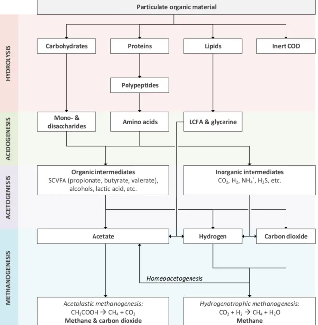
Figure 1: Breakdown of complex organic material to simpler components during anaerobic digestion - process scheme adapted from Gujer & Zehnder (1983); Siegrist et al. (2002); Madsen, Holm-Nielsen &
Esbensen (2011) 6
Figure 2: Block flow diagram depicting the concept of ADM1 16
Figure 3: Parameter estimation procedure typically followed in anaerobic digestion modelling (Donoso-Bravo
et al., 2011) 30
Figure 4: Illustration of the PLSR concept showing dimensions of the data matrices, weight and loading
vectors 35
Figure 5: Schematic showing the main process flow of the full-scale plant. The enclosed section represents
the anaerobic MBR system to which the ADM1 model is configured 40
Figure 6: Schematic describing how COD measurements are differentiated and translated into ADM1 state
variables 44
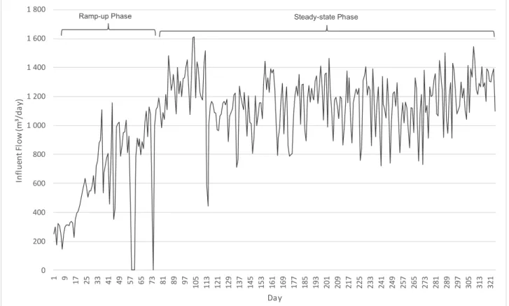
Figure 7: Daily influent volumetric flow into digester, showing the ramp-up period (Day 1 - Day 79) and the
steady-state period (Day 80 - Day 230) 45
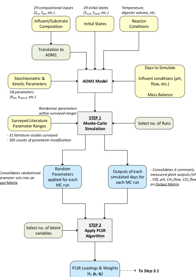
Figure 8: Illustration showing how the PLSR framework is incorporated into the PLS Method. First, the relationship between model parameters and its outputs are mapped as weights and loadings. Thereafter, these PLS constructs are applied to guide parameter calibration. i - no. of latent variables; m - no. of
parameters; p - no. of outputs; t - no. of time intervals simulated. 54
Figure 9: Overview of the PLS Method for ADM1 parameter calibration – Part 1 of 2 60
Figure 10: Overview of the PLS Method for ADM1 parameter calibration – Part 2 of 2 61
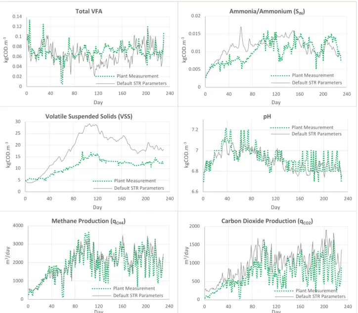
Figure 11: ADM1 simulation using default parameters. Projected values are represented in grey lines and
actual plant measurements are plotted as green dots. 63
Figure 12: Monte Carlo results for VFA, SIN and VSS at 250, 500 and 1500 Monte Carlo runs. The
uncertainty band is represented using mean, 10th, 25th, 75th and 90th percentile values. 65
Figure 13: Monte Carlo results for pH, CH4 and CO2 at 250, 500 and 1500 Monte Carlo runs. The uncertainty
band is represented using mean, 10th, 25th, 75th and 90th percentile values. 66
Figure 14: Maximum and minimum bounds of 1500 Monte Carlo runs for VFA, SIN & VSS before and after
outlier removal 68
Figure 15: Maximum and minimum bounds of 1500 Monte Carlo runs for pH, qch4 & qco2 before and after
outlier removal 69
Figure 16: Evolution of output loading vector (q) for the 1st latent variable 70
Figure 17: Two ADM1 simulations with similar objective function after calibrated using the PLS Method. Green lines represent actual plant measurements; grey lines represent simulation before calibration; solid blue lines represent Method (1)is based on 1500 Monte Carlo runs, no outlier removal and two latent variables; dotted blue lines represent Method (2) which is based on 1500 Monte Carlo runs with outlier
removal and 4 latent variables 71
Figure 18: Model fitting performance at various IQR (extent of outlier removal) and number of latent variables 73
Figure 19: Output RMSE at various outlier removal and number of latent variables 73
Figure 20: Graphical comparison between various parameter calibration methods and residual error plot -
Total VFA 75
Figure 21: Graphical comparison between various model optimisation methods and residual error plot –
Ammonia 77
Figure 22: Graphical comparison between various model optimisation methods and residual error plot - VSS 78 Figure 23: Graphical comparison between various model optimisation methods and residual error plot - pH 79 Figure 24: Graphical comparison between various model optimisation methods and residual error plot – CH4
production 80
Figure 28: Comparing the accuracy of models produced by various parameter calibration methods during
calibration period and validation period. Higher MAPE indicates poorer model accuracy. 86
Figure 29: Comparing the accuracy of models produced by various parameter calibration methods during
calibration period and validation period. Higher MAPE indicates poorer model accuracy 87
Figure 30: Plot showing 500 Monte Carlo simulation runs 129
Figure 31: Plot showing 1000 Monte Carlo simulation runs 129
Figure 32: 250 Monte Carlo simulation runs with outliers beyond ±1.5 x IQR removed 130
Figure 33: 500 Monte Carlo simulation runs with outliers beyond ±1.5 x IQR removed 130
Figure 34: 1000 Monte Carlo simulation runs with outliers beyond ±1.5 x IQR removed 131
Figure 35: 1500 Monte Carlo simulation runs with outliers beyond ±1.5 x IQR removed 131
Figure 36: 500 Monte Carlo simulation runs with outliers beyond ±1.0 x IQR removed 132
Figure 37: 500 Monte Carlo simulation runs with outliers beyond ±3.0 x IQR removed 132
LIST OF TABLES
Table 1: Types of inhibition described in default ADM1 21
Table 2: Corrected default biochemical rate coefficients (νi,j) and kinetic rate equations (ρj) for soluble organic
compounds (Batstone, Keller, Angelidaki, Kalyuzhnyi, Pavlostathis, Rozzi, Sanders, Siegrist & Vavilin, 2002;
Rosen & Jeppsson, 2006) 22
Table 3: Corrected biochemical rate coefficients (νi,j) and kinetic rate equations (ρj) for particulate
components (Batstone et al., 2002; Rosen & Jeppsson, 2006) 23
Table 4: Summary statistics of parameter values surveyed from literature for mesophilic digesters in
comparison to the default values suggested in the ADM1 Scientific and Technical Report 25
Table 5: Number of ADM1 parameter modifications observed during literature survey 28
Table 6: Summary of the NIPALS algorithm for PLSR (Geladi & Kowalski, 1986; de Jong, 1993) 36
Table 7: List of analysed parameters and frequency of analysis 42
Table 8: Comparison of measured data versus the digester’s design basis and various published cheese
whey wastewater characteristics 43
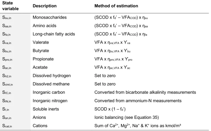
Table 9: Translating full-scale plant data to influent soluble state variables in ADM1 48
Table 10: Definition of terms denoted in Table 9 48
Table 11: Translating full-scale plant data to particulate soluble state variables in ADM1 50
Table 12: Definition of terms denoted in Table 11 50
Table 13: Values specific to the digester modelled in this study 52
Table 14: Description of the 6 outputs/measurands included in the output matrix 56
Table 15: Calibrated ADM1 parameters produced by the various model optimisation methods. Parameters are colour-coded according to the level of sensitivity reported by the STR: Red = high, Blue = medium, Green = low. Values in parenthesis indicate the percentage change from the default STR parameters. 84 Table 16: Ranking of the various parameter calibration methods according to the model’s accuracy during
validation and the duration taken to complete the calibration 87
Table 17: Description of the state variables used in ADM1 models 98
Table 18: Description of the stoichiometric parameters used in ADM1 models 98
Table 19: Description of the kinetic parameters used in ADM1 models 99
ABBREVIATIONS
Glossary DescriptionAD Anaerobic Digestion
ADM1 Anaerobic Digestion Model No. 1
BOD Biochemical Oxygen Demand [mg/l]
CSTR Continuously Stirred Tank Reactor
DS Dry Solids content of the sludge [wt%]
GC Gas Chromatography
HPLC High Performance Liquid Chromatography
IQR Interquartile Range
LCFA Long-Chain Fatty Acids
LHS Latin Hypercube Sampling
MAPE Mean Absolute Percentage Error
MC Monte Carlo
PCA Principal Component Analysis
PCOD Particulate Chemical Oxygen Demand
PCR Principal Component Regression
PLSR Partial Least Squares Regression
RMSE Root Mean Squared Error
SCOD Soluble Chemical Oxygen Demand
SCVFA Short-chain Volatile Fatty Acids
SRT Solids Retention Time
STR Scientific and Technical Report
TCOD Total Chemical Oxygen Demand
VFA Volatile Fatty Acids [mg/l]
VSS Volatile Suspended Solids [mg/l]
WAS Waste-activated Sludge
WWTP Wastewater Treatment Plant
NOMENCLATURE
ADM1 Dynamic State Variablesi Variable Unit Description i Variable Unit Description
1 Ssu kgCOD/m³ Monosaccharides 16 Xli kgCOD/m³ Lipids
2 Saa kgCOD/m³ Amino acids 17 Xsu kgCOD/m³
Monosaccharide degraders
3 Sfa kgCOD/m³ Total LCFA 18 Xaa kgCOD/m³
Amino acid degraders
4 Sva kgCOD/m³ Total valerate 19 Xfa kgCOD/m³ LCFA degraders
5 Sbu kgCOD/m³ Total butyrate 20 Xc4 kgCOD/m³ C4-degraders
6 Spro kgCOD/m³ Total propionate 21 Xpro kgCOD/m³
Propionate degraders
7 Sac kgCOD/m³ Total acetate 22 Xac kgCOD/m³ Acetate degraders
8 Sh2 kgCOD/m³ Hydrogen 23 Xh2 kgCOD/m³
Hydrogen degraders
9 Sch4 kgCOD/m³ Methane 24 XI kgCOD/m³ Particulate inerts
10 SIC kmol C/m³ Inorganic carbon 25 San kmol/m³ Anions
11 SIN kmol N/m³ Inorganic nitrogen 26 Scat kmol/m³ Cations
12 SI kgCOD/m³ Soluble inerts 27 Sh2,g kgCOD/m³ Hydrogen (gas)
13 Xc kgCOD/m³ Composites 28 Sch4,g kgCOD/m³ Methane (gas)
14 Xch kgCOD/m³ Carbohydrates 29 Sco2,g kgCOD/m³
Carbon dioxide (gas)
15 Xpr kgCOD/m³ Proteins
ADM1 Stoichiometric Parameters
Parameter Description Parameter Description
fSI,XC Soluble inerts fraction from
composites fPRO,SU
Propionate fraction from monosaccharides fXI,XC Particulate inerts fraction from
composites fAC,SU
Acetate fraction from monosaccharides fCH,XC Carbohydrates fraction from
composites fH2,AA Hydrogen fraction from amino acids
fPR,XC Proteins fraction from
composites fVA,AA Valerate fraction from amino acids
fLI,XC Lipids fraction from composites fBU,AA Butyrate fraction from amino acids
fFA,LI
Fatty acids fraction from lipids fPRO,AA
Propionate fraction from amino acids
fH2,SU Hydrogen fraction from
monosaccharides fAC,AA Acetate fraction from amino acids
ADM1 Kinetic Parameters
Parameter Unit Description
kdis d-1 Disintegration factor
khyd_CH d-1 Carbohydrates hydrolysis rate constant
khyd_PR d-1 Proteins hydrolysis rate constant
khyd_LI d-1 Lipids hydrolysis rate constant
Ks_IN kmol/m³
Inorganic nitrogen concentration threshold; growth ceases when exceeded
pHUL_acid - pH threshold; no inhibition when pH is above this level
pHLL_acid - pH threshold; full inhibition when pH is below this level
km_su COD.COD-1.d-1
Monod maximum specific uptake rate for monosaccharide degraders
Ks_su kgCOD.m-3 Monod half saturation value for monosaccharide degradation
Ysu COD.COD-1 Biomass yield on uptake of monosaccharides
kdec_xsu d-1 Decay rate constant of monosaccharide degraders
km_aa COD.COD-1.d-1 Monod maximum specific uptake rate for amino acid degraders
Ks_aa kgCOD.m-3 Monod half saturation value for amino acid degradation
Yaa COD.COD-1 Biomass yield on uptake of amino acids
kdec_xaa d-1 Decay rate constant of amino acid degraders
km_fa COD.COD-1.d-1 Monod maximum specific uptake rate for LCFA degraders
Ks_fa kgCOD.m-3 Monod half saturation value for LCFA degradation
Yfa COD.COD-1 Biomass yield on uptake of LCFA
kdec_xfa d-1 Decay rate constant of LCFA degraders
KIh2_fa kgCOD.m-3 Hydrogen inhibitory concentration for LCFA degraders
km_c4 COD.COD-1.d-1
Monod maximum specific uptake rate for valerate & butyrate degraders
Ks_c4 kgCOD.m-3 Monod half saturation value for valerate & butyrate degradation
Yc4 COD.COD-1 Biomass yield on uptake of valerate & butyrate
kdec_xc4 d-1 Decay rate constant of valerate & butyrate degraders
km_pro COD.COD-1.d-1 Monod maximum specific uptake rate for propionate degraders
Ks_pro kgCOD.m-3 Monod half saturation value for propionate degradation
Ypro COD.COD-1 Biomass yield on uptake of propionate
kdec_xpro d-1 Decay rate constant of propionate degraders
KIh2_pro kgCOD.m-3 Hydrogen inhibitory concentration for propionate degraders
km_ac COD.COD-1.d-1 Monod maximum specific uptake rate for acetate degraders
Parameter Unit Description
KInh3_ac kgCOD.m-3 Free ammonia inhibitory concentration on acetate degraders
pHUL_ac -
pH threshold; no inhibition on acetate degradation when pH is above this level
pHLL_ac -
pH threshold; full inhibition on acetate degradation when pH is below this level
km_h2 COD.COD-1.d-1 Monod maximum specific uptake rate for hydrogen degraders
Ks_h2 kgCOD.m-3 Monod half saturation value for hydrogen degradation
Yh2 COD.COD-1 Biomass yield on uptake of hydrogen
Kdec_xh2 d-1 Decay rate constant of hydrogen degraders
pHUL_h2 -
pH threshold; no inhibition on acetate degradation when pH is above this level
pHLL_h2 -
pH threshold; full inhibition on acetate degradation when pH is below this level
CHAPTER 1
INTRODUCTION
1.1. Background
Anaerobic digestion (AD) has remained the mainstream approach for treating high strength organic waste since its invention as a waste/wastewater treatment technology. Its application is wide: ranging from municipal wastes such as municipal solid wastes and sewage sludge to industrial wastes such as livestock manure and food processing wastewater. Co-digestion of municipal wastes in combination with industrial wastes is also a well-accepted application (Angelidaki & Ellegaard, 2003).
Contrary to aerobic biological processes, anaerobic digestion can operate at significantly higher organic loading rates (i.e. more compact), produces lesser sludge as well as recovers energy from the waste as biogas (McCarty, 1964). These advantages are undeniably attractive to the industries because on-site space designated for waste treatment is often limited; plus the ever-increasing drive to reduce utility costs, and to create an environmentally sustainable image. Being a low energy-intensive process, the treatment plant is generally net energy positive, meaning that excess energy could be repurposed for other users in the form of either electricity or heat/steam. Another major cost-saving, which often left unaccounted for, is the disposal cost and penalties that would otherwise be incurred if no treatment was undertaken.
In spite of the benefits, modern anaerobic digestion plants still rely heavily on human monitoring and inputs due to lack of affordable advanced instrumentations. Anaerobic processes, in contrast to aerobic processes, require operators with higher technical abilities because the system is more susceptible to process upsets (Madsen, Holm-Nielsen & Esbensen, 2011). A severe process failure would require long periods to recover, and the financial impact of such a scenario remains the primary concern of adopting this technology (McCarty, 1964). To reduce risk, designers tend to undertake a conservative approach by selecting a lower organic loading rate intentionally (i.e. oversizing the digesters). This approach results in design redundancy and capital wastage.
Nonetheless, by 2007, there was already more than of 2250 anaerobic digestion plants implemented globally for treating industrial type wastewater (Van Lier, 2008). The field of application continues to broaden thanks to the immense research effort on the microbial, biochemical and physicochemical mechanisms within AD. It has led to the development of higher-rate reactors, wider digester operating temperature ranges and advancement in modelling and process control techniques. (Costello, Greenfield & Lee, 1991; Ge, Jensen & Batstone, 2011; Jimenez et al., 2015).
1.2. Research Motivation and Rationale
Troubleshooting a full-scale anaerobic digestion plant is not straightforward; generally relies on operational experience and a trial and error approach. The difficulty is attributed to a lack of on-line process monitoring, automated diagnosis and management. Online instruments commonly employed on industrial scale are basic in functionality because advanced instruments are expensive, intricate and require a higher level of maintenance and calibration (Steyer et al., 2002; Vanrolleghem & Lee, 2003).
Many useful data are acquired through manual sampling followed by offline analysis in a laboratory. Some constituents may be analysed on- site if simple and economical to perform, but others may require an external better-equipped laboratory. This process is cumbersome and does not allow the reactor to be managed via dynamic feedback; instead, it relies entirely on the plant operators’ experience (Madsen et al., 2011; Spanjers & Lier, 2006). Moreover, many sites do not have dedicated technical personnel to interpret the collected data correctly.
A process diagnosis & management tool, based on basic on-site obtainable data as inputs, would be highly valuable. The tool could be designed to foresee instability and to initiate corrective actions. Furthermore, since most existing digesters were designed rather conservatively, this tool would allow one to operate above the initial design set-points and exploit the true effective capacity of the digester (Liu, Olsson & Mattiasson, 2004). Developing such a tool before the advent of affordable advanced instruments would, otherwise, first require a reasonably accurate model.
Several mathematical models have been developed for AD process modelling. Despite differences in model structure and number of biochemical conversion processes incorporated, accuracy of the model outputs are fundamentally governed by the values that are assigned as the stoichiometric and kinetic parameters. Parameter calibration is thus an important step in model development.
Models with higher degrees of sophistication generally feature higher number of parameters. For instance, the most widely used model of recent years called Anaerobic Digestion Model No. 1 (ADM1) has 58 parameters by default. The high degrees of freedom mean that the calibration process can become extremely time-consuming if the parameters are adjusted one at a time. As such, sensitivity analysis techniques or expert knowledge are commonly employed to reduce the degrees of freedom. There is currently no common protocol regarding parameter calibration. Selection of parameters to be calibrated relies largely on the modeller’s discretion. A method that is free from modeller’s bias could offer a standardised way to calibrate ADM1 parameters.
Partial Least Squares Regression (PLSR) is a popular statistical tool used in chemometrics to identify and to regress the non-linear relationship between two matrices as a linear model. It is envisaged that this tool could present a methodical way to relate ADM1 parameters and the model outputs. An integral part of PLSR is dimensionality reduction. This means that a large number of model parameters could potentially be transformed into a smaller subset called latent variables, and simplify the calibration process due to the reduced degrees of freedom. In theory, a reduction in bias avoids overfitting.
Soft sensors have a prospective role in industrial AD plant operation. Using online measurements from conventional field sensors as inputs to a process model, a soft sensor allows other valuable process measurements that are expensive (e.g. microbial species) or time-consuming to analyse (e.g. VFA species) to be predicted instead. Access to this information would empower advanced monitoring and control strategies that further enhance the digester’s stability.
As pointed out in a review paper by Jimenez et al. (2015), research involving soft sensoring generally utilise simplified models instead of ADM1. Simplified models can predict basic lumped measurements (e.g. total COD, VFA, etc.) which are appropriate for basic plant control, but inadequate for ultimate soft sensor development as it lacks the level of sophistication that ADM1 provides. Challenges that ADM1 faces are the high degrees of freedom and the model’s requirement for detailed substrate composition. As ADM1 remains the forefront of AD modelling research, the ultimate goal should be aimed at addressing these challenges such that ADM1 is compatible for soft sensor applications.
1.3. Research Aim and Limitations
This research aims to develop a parameter calibration method that could be included in the ADM1 framework. The method shall adopt the concepts of PLSR and demonstrate whether model optimisation can be achieved without the need to manually select parameters for calibration. Performance of this method shall be benchmarked against other calibration methods.
The data available for the modelling demonstration in this thesis were sourced from the operational data log of an industrial-scale AD plant. Additional in-depth characterisation tests or change to sample frequency were not possible because access to the plant is restricted. Analytical constraints are normal for industrial applications due to affordability reasons (Arnell et al., 2016). This limitation, however, did not impede the research objectives because the research focuses on framework development rather than the fit accuracy. In fact, for an industrial setting, high accuracy of every model outputs may not be unnecessary, as models are used for assessing changes in output trends (Batstone & Keller, 2003).
1.4. Research Questions and Objectives
1.4.1. Research Questions
1. How can the concept of Partial Least Squares Regression be exploited for parameter calibration? 2. What are the procedures when applying this method for industrial-scale anaerobic digestion
modelling?
3. Is this method capable of simplifying the calibration process and avoid over-calibration?
• Translate experimental data obtained from an industrial-scale digester into the format required by ADM1
• Conduct a literature survey for stoichiometric and kinetic parameter values to establish the variance in each parameter
• Perform Monte Carlo simulation using the surveyed information to generate input and output data set • Identify latent relationships between model parameters and outputs using PLSR algorithm and data
set generated from Monte Carlo simulation
• Attempt parameter calibration by using the latent relationships as guidance • Benchmark the new calibration method against other calibration methods
CHAPTER 2
LITERATURE REVIEW
2.1. Anaerobic Digestion Theory
2.1.1. Fundamental Biochemical Reactions Hydrolysis
Hydrolysis (also referred to as solubilisation) involves the disintegration of complex, insoluble polymeric matter by extracellular enzymes into structurally smaller products. In this step, as illustrated in Figure 1, carbohydrates, proteins and lipids are broken down predominantly into monosaccharides, amino acids and LCFAs, respectively (Heukelekian, 1958). Being soluble, these products can enter the biomass and undergo further breakdown intracellularly. Carbohydrates were found to hydrolyse faster than proteins and lipids (Eastman & Ferguson, 1981).
Acidogenesis
The process of acidogensis (also referred to as fermentation) follows hydrolysis. In this step, acidogens convert monosaccharides into predominantly low molecular weight VFAs such as acetate, propionate and butyrate, lactic acid, H2 and CO2 (Gujer & Zehnder, 1983). Lactic acid is an intermediary compound that converts rapidly
into VFAs; however, it could potentially accumulate within the digester when a high load of readily degradable substance such as glucose (Costello et al., 1991) is received. The acidification products of amino acids are higher molecular weight VFAs such as i-butyrate, valerate and i-valerate, H2, CO2, ammonium and sulphides.
Hydrogen production is mostly related to the acidification of monosaccharides rather than amino acids. For proteinaceous substrates, hydrolysis is regarded as the rate-limiting step because the rate of fermentation is considerably faster (Pavlostathis & Gossett, 1988). Yu & Fang (2001) further observed, in a study on dairy wastewaters, that carbohydrates tend to suppress the degradation of proteins. This causes carbohydrates to acidify preferentially and more rapidly in comparison to proteins and lipids.
Fermentation pathways of LCFAs depend on the carbon structure of the acids. If the acid has an odd number of carbon atoms, both acetate and propionate will form. However, if the acid has even carbon counts, acetate is the only short-chained VFA that will be formed (McInerney & Bryant, 1981). Another fermentation product is molecular hydrogen. Hydrogen serves as a sink for the electrons liberated when LCFAs are oxidised (Gujer & Zehnder, 1983).
Acidification favours the VFA and hydrogen production pathway when the substrate COD concentration is low. However, at a higher COD concentration, the pathway would shift towards alcohols such as propanol and
explained this metabolic shift as a mechanism for acidifiers to counter the VFA build-up and consequential pH inhibition. The pathway change is reported to trigger only when acetate or butyrate exceed a threshold concentration of 0.4 - 0.6 g/l (Jones & Woods, 1986).
Figure 1: Breakdown of complex organic material to simpler components during anaerobic digestion - process scheme adapted from Gujer & Zehnder (1983); Siegrist et al. (2002); Madsen, Holm-Nielsen & Esbensen (2011)
Acetogenesis
According to McCarty & Smith (1986), the conversion from ethanol and propionate to acetate and hydrogen requires a Gibbs free energy ΔGo’ of 9.65 kJ/mol and 71.67 kJ/mol, respectively (Equation 1 & Equation 2).
Conversion of other intermediate VFAs such as butyrate and valerate also holds positive free energy. This fact implies that these reactions will remain non-spontaneous until acetate and/or hydrogen concentrations are low enough to induce a negative free energy.
Hydrogen is consumed by H2-utilising bacteria during methanogenesis to produce methane. Under sufficiently
low hydrogen level, acidogens are observed to deviate from the ethanol (C2H6O) production pathway because
ethanol acts as an electron sink. Instead, H2 is produced from the oxidation of NADH, a process which leads
to a preferential formation of acetate (C2H3O2-) (Wolin, 1982). The production ratio between acetate and
ethanol is therefore dependent on the concentration of H2-utilising methanogenic bacteria present during
fermentation.
Oxidation of ethanol: !"#!"$%" + "$% → !"#!%%(+ ")+ 2"$ Equation 1
Oxidation of propionate: !"#!"$!%%(+ 2"$% → !"#!%%(+ 3"$+ !%$ Equation 2
Methanogenisis
Methanogensis refers to the final carbon degradation step in which methane gas is produced. This process only occurs when all alternative forms of electron acceptors (e.g. O2, NO3-, SO42-,) are depleted. Two major
pathways are well known: (i) the uptake of acetic acid by acetoclastic methanogens; and (ii) the reduction of carbon dioxide by hydrogenotrophic methanogens.
The first pathway, termed acetolastic methanogenesis, follows the oxidation of acetate into carbon dioxide and methane (Equation 3). In the second pathway, termed hydrogenotrophic methanogenesis, methane is formed through the reduction of carbon dioxide by hydrogen (Equation 4). This pathway takes place only when acetate is depleted and carbon dioxide left as the sole electron acceptor. Theoretically, up to a third of the total methane could be produced via this route (Conrad, 1999).
!"#!%%" → !",+ !%$ Equation 3 1 2!%$+ 2"$→ 1 2!",+ "$% Equation 4
Hydrogenotrophic methanogenesis serves as an important sink for reducing hydrogen concentration in the digester. If hydrogen is allowed to accumulate, for example, due to suppressed methanogenic activity, fatty acid degrading organisms will become inhibited and initiate the reduction of low molecular VFAs (i.e. acetate, propionate) into alcohols and higher molecular VFAs (i.e. butyrate). This impedes methane production consequently because methanogens utilise products from acetogenesis as substrates (McInerney & Bryant, 1981).
On the contrary, if hydrogen is effectively consumed and kept below the inhibitory level, hydrogen production will regulate in conjunction with the hydrogen partial pressure (Pavlostathis & Giraldo-Gomez, 1991). Sustaining the syntrophy between acetogenic organisms (which produces hydrogen) and hydrogenotrophic methanogens (which consumes hydrogen) is therefore crucial for efficient AD operation.
Sulphate Reduction
Under anaerobic conditions, sulphate will be reduced to sulphide first before methane production occurs. The reason is that the biological reduction of sulphate is slightly more thermodynamically favoured than methanogenesis. The reaction (Equation 5) is mediated by sulphate reducing bacteria (SRB) which competes for the same electron donors as methanogens, and as a consequence, lesser acetate and hydrogen are available for methane production (Kalyuzhnyi & Fedorovich, 1998). Theoretically, 0.67 mg/l of COD is required to reduce 1 mg/l of sulphate (Liamleam & Annachhatre, 2007).
!"#!%%(+ .%,$(→ ".(+ "!%#( Equation 5
Denitrification
Nitrate will undergo a series of reduction processes, termed denitrification, when subject to anaerobic conditions. Facultative anaerobic bacteria tend to use nitrate as an electron acceptor because the reduction reaction is highly favoured thermodynamically. During denitrification, nitrate is converted into ammonia and nitrogen gas, via nitrite as an intermediate (Tiedje, 1988).
The conversion path to ammonia, called ammonification, is a selective process that depends on the ammonia concentration. Under ammonia-limiting or nitrate-limiting conditions, ammonifiers compete well against denitrifiers which mediate the reduction of nitrate (Equation 6) and nitrite (Equation 7). As the reduction process utilises organic carbon, the theoretical COD required for (or loss due to) denitrification is 2.86 mg/l and 1.71 mg/l per mg/l of NO3 and NO2, respectively (Akunna, Bizeau & Moletta, 1992). This fact effectively implies that
methane gas production will decrease when denitrification occurs.
/%#(+ 5 24C3H5$O3+ H$O → 1 2/$+ 5 4!%$+ 7 4"$% + %"( Equation 6 /%$(+ 1 8C3H5$O3+ H$O → 1 2/$+ 3 4!%$+ 5 4"$% + %"( Equation 7
2.1.2. Anaerobic Digestion Kinetics
Kinetics are key factors when developing dynamic models. They describe the rates of biomass growth, substrate uptake, product formation and microbial decay during biochemical reactions. Good understanding of microbial decay kinetics is particularly essential for anaerobic digestion because specific growth rates are much lower than aerobic processes (Pavlostathis & Giraldo-Gomez, 1991).
Several mathematical equations have been derived to describe biological growth kinetics. In general, they are based on the relationship between growth rate and substrate concentration. The kinetic model applied in ASM (Activated Sludge Model) is the Monod equation (Monod, 1942). It has further found success in describing anaerobic digestion processes other than the hydrolysis process which is best modelled by first-order kinetics.
The Monod equation describes microbial growth by relating it to the growth-limiting substrate’s concentration (Equation 8). Parameters such as μmax and Ks are empirical, which are obtained by fitting the observed
substrate utilisation data using non-linear regression (Robinson & Tiedje, 1983). These parameters can differ between different studies even if the substrate is similar. Pavlostathis & Giraldo-Gomez (1991) explained this variability as a result of difference in mode of operation (batch or continuous) and/or operating conditions (e.g. temperature, pH) applied during each study.
: = :<=>
.
?@+ .
Equation 8
where:
μ is the specific microorganism growth rate [d-1];
μmax is the maximum specific microorganism growth rate [d-1];
S is the limiting substrate concentration [kgCOD.m-3];
Ks is the half-saturation constant;
From the Monod equation, the substrate uptake rate (km) can be calculated by relating the growth rate to the
biomass yield ratio (Equation 9).
A<= :<=>B Equation 9
2.1.3. Toxicity & Inhibition
Toxicity related to pH is the most commonly encountered form of toxicity. It is caused by the presence of weak acids e.g. hydrogen sulphide (H2S) and unionised VFAs, and weak bases e.g. unionised ammonium. Other
forms of toxicity, such as biocides and heavy metals, are described further in the literature by van Haandel and van der Lubbe (2007).
Sulphides are formed when sulphate ions are reduced during methanogenesis or when sulphur-containing amino acids (cysteine and methionine) are degraded. H2S, which is a toxin for methanogenic bacteria, exists
in equilibrium with HS- whereby their concentrations are functions of pH (Equation 10). The pKa value of the
H2S/HS- equilibrium is 6.99 at 30°C. This implies that at a pH of 6.99, 50% of the sulphides will be in the H2S
form and increasing concentrations at lower pH values.
"$. ↔ ".(+ ") Equation 10
Although each VFA has different pKa values, VFA exists predominantly in the unionised form at lower pH
values. Unionised VFAs are considered toxic because it can diffuse through the cell membrane and cause cell lysis due to a large internal pH drop as it dissociates within. The loss in microbial activity inhibits the degradation of hydrogen and organic acids (Siegrist, Renggli & Gujer, 1993).
An easily acidifying substrate with high organic content could lead to rapid accumulation of acetic acid. Unless sufficient alkalinity buffer is present or corrective action taken to reduce the influent loading rate, the decrease in pH will amplify the above-mentioned inhibition effects.
Ammonia is generated when the protein component of a waste is digested. Given the fact that NH3/NH4+
equilibrium has a pKa of 9.3 at 25°C, ammonia toxicity is only a concern at high pH where the unionised form prevails. Microbial activity is reported to be inhibited when the free NH3 level reaches 150 mg/l (Braun, Huber
& Meyrath, 1981).
2.1.4. Commonly Monitored Process Indicators
This section discusses the relevance of measurements commonly monitored at an industrial-scale AD plant. Except for pH, temperature and volumetric flow rates, most of the measurements are off-line analyses from manually taken samples. Feedback control strategies are thus limited due to the long measurement delay. In spite of significant advancement made in recent years to develop sensors that allow in-situ measurements, affordability remains a major obstacle to the deployment of advanced instruments at industrial plants in developing countries (Jimenez et al., 2015).
COD
Chemical Oxygen Demand (COD) indicates the generic pollution strength within a wastewater stream. It refers to the amount of oxygen required to completely oxidise the organic material present. Total COD (TCOD) is a term used to describe the COD content of a well-mixed wastewater sample inclusive of all entrained solids. Soluble COD (SCOD) refers to the COD of a filtered or centrifuged wastewater sample, whilst the contribution of the suspended solids to TCOD is referred to as particulate COD (PCOD). The relationship between the terms is described in Equation 11.
D!%E = .!%E + F!%E Equation 11
TSS & VSS
Total Suspended Solids (TSS) indicates the total quantity of suspended, or non-filterable, solid particulates in a wastewater stream. Closely related to TSS is the Volatile Suspended Solids (VSS) component which describes the concentration of volatile solid particulates. When a sample is taken from the digester, VSS represents the organics content within both influent waste and biomass; however, given a highly soluble digester feed, the VSS concentration is an approximate quantitative measure of the biomass sludge inventory within the digester. This information allows one to control the food-to-microorganism (F/M) ratio and to detect biomass loss due to wash-outs.
In anaerobic digestion, little energy is allocated to cell growth and therefore the yield/growth of anaerobic biomass – particularly LCFAs, acetate and propionate degraders - is considerably slower compared to aerobic oxidation process (McCarty & Smith, 1986; Siegrist et al., 1993). This fact further emphasizes the importance of tracking VSS in maintaining digester stability.
Inert, or non-biodegradable, particulates such as inorganic precipitates (calcium carbonate, struvite, etc.) may enter the digester as part of the substrate feed or form within the digester. Its concentration is calculated as the difference between the measured TSS and VSS concentrations.
pH & Alkalinity
pH indicates how acidic or basic an aqueous solution is, and is defined as the negative logarithm of hydrogen ion concentration (Equation 12). pH is regarded as an important parameter because some constituents (e.g. H2S, NH3) that are known to induce microbial toxicity or inhibition exists in equilibria relative to other harmless
species. Fractional amounts of each species change as a function of hydrogen ion concentration. Key equilibria of relevance in AD research are the carbonate equilibrium (CO2/HCO3-/CO3), hydrogen sulphide equilibrium
(S2-/HS-,H2S), ammonium equilibrium (NH4+, NH3) and VFA equilibrium.
G" = − log5L[")] Equation 12
Alkalinity is a measure of the digester’s pH buffering capacity and a key control parameter for steady digester functioning (McCarty & Smith, 1986). Without adequate buffering, a sudden pH drop will occur when VFA formation outpaces its metabolism rate, resulting in pH related toxicity. This occurrence is common, particularly during transient conditions. External alkalinity (e.g. lime or caustic soda) could be added as a countermeasure. The carbon dioxide-bicarbonate system serves as the main pH buffering mechanism for anaerobic digestion (Equation 13 & Equation 14). Alkalinity is naturally formed through the production of CO2 during the metabolism
of VFAs, which then converts to bicarbonate. A portion of the produced CO2 is stripped to the biogas as
gaseous CO2, whilst most of the CO2 remain dissolved in the liquid as bicarbonate HCO3-. The stripping
process is the primary contributor to alkalinity recovery during anaerobic digestion.
!%$+ "$% ↔ "$!%# Equation 13
"$!%#↔ "!%#(+ ") Equation 14
Another source of alkalinity is ammonia, which is produced when protein or organic nitrogen in the feed substrate is mineralised during the digestion process (van Haandel & van der Lubbe, 2007). The subsequent formation of ammonium carbonate serves as alkalinity (Equation 15). Products of sulphate reduction reaction also contribute to alkalinity (Equation 5).
/"#+ "$% + !%$→ /","!%# Equation 15
Excess amounts of VFAs are toxic to methanogenic bacteria. In a well-buffered system, pH measurements will fail to detect the accumulation of VFAs because pH change would occur only when alkalinity is close to depletion (Hawkes et al., 1993). A popular monitoring strategy employed on industrial is to maintain a good ratio of VFA relative to alkalinity, which is known as the Ripley’s ratio (Ripley et al., 1986).
VFA
Total VFA level has been widely reported as a reliable process status indicator (Madsen et al., 2011). According to Boe et al. (2010), a good understanding of individual VFA constituents (n-butyric, iso-butyric and propionate in particular) could provide even better insight on the digester’s stress level and potentially act as a precautionary indicator towards process imbalance.
Measurement of individual VFA constituents is conventionally performed off-line using gas chromatography or high-performance liquid chromatography (HPLC) methods. Development of automated online devices for continuous measurement on industrial-scale plants are not yet mature in terms of affordability and robustness (Jimenez et al., 2015). Nonetheless, the advantage of online VFA measurement is well acknowledged and much interest has been vested in its research and development.
Temperature
The operating temperature in anaerobic digesters has a prominent effect on the degradation efficiency and biogas production. In most cases, an increase in temperature up to 42 °C, will lead to improved performance (Donoso-Bravo et al., 2009; Rebac et al., 1995). The reason is that kinetic rates and equilibrium coefficients which governs biochemical reactions and physicochemical processes including gas-liquid transfer are all functions of temperature. Temperature influence on biogas production is approximately 3.4% per degree from 25 - 30°C and 1.6% per degree from 30 - 35°C (Bergland, Dinamarca & Bakke, 2015).
For digesters operating in the mesophilic temperature range, the influence of temperature on biochemical reactions and physicochemical processes can be corrected by the double Arrhenius equation (Equation 16) and van’t Hoff equation (Equation 17) respectively, according to Batstone (2006).
O = P5 QRG S −T=5 UD V − P$ QRG S −T=$ UD V Equation 16 where:
ρ is the microbial activity;
A is the pre-exponential constant (empirical); Ea is the apparent activation energy [J.mol-1];
R is the universal gas constant [J.K-1.mol-1];
T is the absolute temperature [K]
WX?$ ?5= ∆"° U S 1 D5− 1 D$V Equation 17 where:
K1, K2 are the equilibrium constants before and after temperature-correction respectively;
∆H° is the enthalpy change [J.mol-1];
2.2. Overview of Anaerobic Digestion Modelling Development
Key milestones in anaerobic digestion modelling are listed in a review by Donoso-Bravo et al. (2011). This section reviews some of the milestones in greater detail, as these models contributed to the development of the Anaerobic Digestion Model No. 1 (ADM1). A comprehensive list of all AD models is provided in review papers by Appels et al. (2008) and Lauwers et al. (2013).
2.2.1. Two-microbial-culture model
In 1977, Hill & Barth (1977) developed a mathematical model to simulate the digestion process of animal waste. The development was motivated by the benefits that a dynamic model would allow one to study the digester’s stability when it is subjected to different operating conditions.
The model considers only two microbial groups, namely acid-formers and methane-formers, to be responsible for the conversion of organics to VFAs and from VFAs to methane gas respectively. Other variables accounted in the model are commonly analysed parameters such as volatile matter/solids, VFAs, soluble organics, cations, carbon dioxide and ammonia. This model assumes the stoichiometry of soluble organics to be the same as glucose, and that VFAs is broadly representable as acetic acid.
Variables are represented by a set of multiple non-linear differential equations that ensure mass and charge balances are maintained continuously. All insoluble organics must be solubilised first before it is amenable to degradation. This conversion is simply based on a 1:1 stoichiometry and is not subjected to any kinetic rates. The only inhibitor taken into account by the model is the presence of unionised ammonia on the growth of methane-formers.
All kinetic and physicochemical constants applied for the model were sourced from previous investigation works related to similar waste substrate, and no parameter calibration was made. For model validation, the author selected four variables which were deemed most important for animal waste digestion, namely methane gas, volatile matter/solids, VFAs and alkalinity. For the steady-state period the model was found capable of fitting actual experiment data with reasonable accuracy but failed to predict well during transient periods.
2.2.2. Steady-state acid phase model
A study by Eastman & Ferguson (1981) pointed out the likelihood of the acid phase, which consists of the hydrolysis of particulates to soluble organics and the subsequent fermentation to VFAs, to be the rate-limiting step during anaerobic digestion. In retrospect, earlier models (Andres, 1969; Graef & Andrew, 1974) considered acetolastic methanogenesis as the rate-limiting step and thus did not include any acid phase mechanisms.
Hydrolysis, in particular, was reported to be a potential rate-limiting step in anaerobic digestion, especially when digesting particulate organic substances. The overall digestion rate could be constrained during periods
understanding the composition make-up between particulate and soluble organics is regarded as crucial for establishing the rate-limiting factor in context. This fact was well supported by other researchers (Gujer & Zehnder, 1983; Pavlostathis & Gossett, 1988).
The acid phase model includes a first-order function to describe the hydrolysis step and Monod’s equation to describe the growth of acid-formers (in association with the utilisation of soluble organics). Recognising that different particulates within a complex substrate could hydrolyse at dissimilar rates, a first-order function was proposed as the most appropriate method to describe the lumped/effective hydrolysis effect.
The research confirmed robustness of the acid phase across a wide range of pH and/or solids concentration. Following the “two-phase digestion” approach proposed by Pohland & Ghosh (1971) where two separate reactors are operated in series but under different conditions, Eastman & Ferguson (1981) proved that the digester’s stability can be greatly improved when each reactor is operated at conditions most optimally suited for the acid-forming bacteria and methanogenic archaea.
2.2.3. Dynamic single-stage high-rate anaerobic reactor model
A major advancement in anaerobic modelling was presented in the work by Costello et al. (1991). Using the model framework developed by Mosey (1983), this model introduced the effects of hydrogen inhibition, product inhibition, and most notably, a larger ecosystem of anaerobic bacteria which are fundamentally involved in the degradation process. Unlike prior models which only considered a single acidogenic step to form acetic acids, this model accounts for intermediate volatile acids such as propionic and butyric acids as well.
A unique development made by the author was to incorporate a comprehensive set of inhibition and regulation functions into the model structure. It is implemented by multiplying the relevant inhibition functions to a substrate’s utilisation rate formula as described by Monod’s equation. The inclusion of inhibition and regulation effects based on hydrogen gas concentration in the biogas is an important feature of this model.
Inhibition functions influence substrate uptake rates of acidogens and acetogens, whilst regulation functions modify the production rates of the acidifiers’ end-products (propionic acid, butyric acid, acetic acid and lactic acid). Other inhibitory phenomena built into the model were:
• Individualised pH inhibition function for each type of bacteria - glucose, lactic acid, propionic acid and butyric acid
• Product inhibition effect as a result of product accumulation and high product-to-substrate ratio:
- A competitive inhibition function was proposed for propionic acid and butyric acid bacteria. Only acetic acid is considered as the cause of inhibition. VFAs, including lactic acid, were deemed non-influential
- A non-competitive inhibition function was proposed for glucose and lactic acid bacteria. VFAs are the cause of inhibitory products.
2.2.4. Development of higher complexity models
Angelidaki et al. (1993) enhanced the model initially developed by Hill & Barth (1977), with the intention to simulate free ammonia inhibition on methanogens more accurately. This improvement is critical for digesters treating substrates containing high protein or ammonia in particular. As free ammonia concentration depends on pH and temperature the research focused on improving pH prediction and the temperature correction of dissociation constants. According to the authors, free ammonia inhibition could recover spontaneously and prevent system failure. It was reported that as VFAs accumulates, the reduction in pH would cause a shift in ammonia equilibrium, resulting in lower free ammonia concentration.
One of the first universal non-substrate specific models was created by Vavilin et al. (1994). The model is intentionally simplified to describe key anaerobic steps only, where carbohydrates, proteins and lipids are lumped as a single hydrolysed substrate term, while propionate served as the only fatty acid intermediate. Despite having a simplified structure the model included decay mechanisms for dead biomass to assimilate back to the ecosystem as degradable and non-degradable components. The inclusion of extra processes, such as sulphate reduction and syntrophic methanogenesis, further adds sophistication to this generic model. The sulphate reduction process involves the conversion of sulphates into sulphides, with acetate and propionate as substrates. Consequently, sulphate reducing bacteria are added to the model’s ecosystem.
2.3. Anaerobic Digestion Model No. 1 (ADM1)
2.3.1. Introduction
In 1997, the IWA Task Group for Mathematical Modelling of Anaerobic Digestion Processes was formed with the task to create a generic anaerobic digestion model. Developed by international experts from different anaerobic digestion modelling backgrounds the model intends to provide a common basis – in terms of the model structure, process mechanisms and nomenclature – for future modelling research such that collaboration and validation of results are possible. The model was published in 2002, under volume 13 of IWA Scientific and Technical Report (STR), as “Anaerobic Digestion Model No.1 (ADM1)”.
Figure 2: Block flow diagram depicting the concept of ADM1
The default/original version of ADM1 model features 29 dynamic state variables (Table 17). These variables represent 26 constituents present in the liquid phase, of which 14 are soluble and 12 are particulate, as well as 3 gas phase constituents within a CSTR system. State variables in the outlet streams are outputs calculated from the model’s differential mass balance equations which describe the biochemical and physicochemical reactions taking place inside the digester. The conversion rate and kinetics of each reaction are governed by stoichiometric and kinetic parameters listed in Table 18.
2.3.2. Nomenclature and Units
Refer to Table 17 – Table 19 in the Appendix for definition of the nomenclatures used in ADM1.
Influent
Flow (qin)
26liquid compositions (Ssu,in, Saa,in, etc.) 3 gas compositions (Sh2_g,in , SCH4_g,in , etc.)
Gas
Flow (qgas)3gas compositions (Sh2_g,out , SCH4_g,out , etc.)
Liquid
Flow (qout)26liquid compositions (Ssu,out, Saa,out, etc.)
Dynamic CSTR System (DAE mass balance solver) Gas Phase
Liquid Phase
19biochemical & physico-chemical reactions
58stoichiometric & kinetic parameters (Kdis, khyd,ch, etc.)
Reactor Specifications
(Temperature, digester volume, etc.)