An Extreme Value Approach to Modeling Risk of Extreme Rainfall in Bangladesh

Lund Univeristy, Faculty of Science, Mathematical Statistics

Bachelor thesis in Mathematical Statistics

An Extreme Value Approach to Modeling

Risk of Extreme Rainfall in Bangladesh

Authors :

Emmy Andersson

Evelina Nilsson

Supervisor :

Nader Tajvidi

May 7, 2018

Abstract

The extreme value theory has been applied on daily rainfall in the five most exposed areas of Bangladesh between the years 1980-2016 in order to esti-mate extreme rainfalls for the next 10, 50 and 100 years. These types of computations are necessary for optimising planning and preparations for ex-treme future rainfalls which can lead to minimising property damage and ultimately saving lives.

Generalised extreme value distribution is fitted to annual maxima accord-ing to the block maxima method. In addition, the generalised Pareto distri-bution is fitted to the daily rainfall according to the Peaks-Over-Threshold method. The different parameters were estimated with a 95 % confidence interval both through the delta- and the profile likelihood methods. There-after, the return period is computed according to each model using the same estimated confidence intervals.

Popul¨

arvetenskaplig sammanfattning

Extremv¨ardesteori har applicerats p˚a daglig nederb¨ord i Bangladesh, mel-lan 1980-2016, fr˚an fem av de mest utsatta omr˚adena f¨or att ber¨akna den f¨orv¨antade nederb¨orden de kommande 10, 50 och 100 ˚aren. Denna typ av ber¨akningar ¨ar v¨asentliga f¨or att kunna vidta ˚atg¨arder som i sin tur minskar skador p˚a egendom och framf¨orallt r¨addar liv.

Generaliserad extremv¨ardesf¨ordelning har anv¨ants f¨or att anpassa ˚arligt max-ima enlig block maxmax-ima-modellen. Aven generaliserad Pareto f¨¨ ordelning anv¨ands f¨or att anpassa den dagliga nederb¨orden enligt peaks over threshold-metoden. De olika parametrarna skattades med ett 95 % konfidensintervall genom b˚ade delta- och profile likelhood-metoden. D¨arefter ber¨aknades den f¨orv¨antade nederb¨orden med b˚ada tidigare n¨amnda modeller, ¨aven dessa med ett 95 % konfidensintervall.

Acknowledgement

We would first like to give a special thank you to our supervisor Nader Tajvidi for all his help through this project. He has been a great support throughout the whole process.

We would also like to thank Nasrine Sultana for providing us with all the necessary data and articles for this research.

Contents

1 Introduction 5

2 Theory 7

2.1 Generalized extreme value distribution (GEV) . . . 7

2.1.1 Block size selection . . . 9

2.1.2 Return level . . . 10

2.1.3 Inference for GEV distribution . . . 10

2.2 Generalized Pareto distribution (GPD) . . . 11

2.2.1 Threshold selection . . . 13 2.2.2 Return level . . . 14 2.2.3 Inference of GPD . . . 16 2.3 Model Diagnostic . . . 16 2.3.1 Probability plot . . . 16 2.3.2 Quantile plot . . . 17

2.4 Probable maximum rainfall . . . 17

3 Methodology 18 3.1 Data . . . 19

3.2 Block-size selection for GEV . . . 21

3.3 Threshold selection for GPD . . . 22

4 Rainfall pattern for the different stations 26 4.1 Barisal . . . 26 4.2 Chandpur . . . 26 4.3 Satkhira . . . 26 4.4 Madaripur . . . 26 4.5 Faridpur . . . 27 5 Results 28 5.1 Parameter estimation for extreme rainfall . . . 28

5.2 Return level for extreme rainfall . . . 31

5.3 Probable maximum rainfall . . . 34

6 Conclusions 35

1

Introduction

Bangladesh is a country in southern Asia that often experiences heavy flood-ing due to its geographical location as well as its flat and low level landscape. The country is located on a latitude subject to tropical monsoon climates which brings heavy rainfall to the area. Brahmaputra and Ganges are two large rivers running through the country creating large areas of river delta flowing into the Bay of Bengal. The heavy rainfall that can be experienced during just a few hours leads to devastating consequences for the population, making Bangladesh one of the most vulnerable countries to flooding, [6]. Global warming has also a major effect on the amount of rain Bangladesh experiences. According to IPCC AR:5 Bangladesh is expected to have a 5 % increase of rainfall by year 2030, [8]. Between years 1996-2015 there were 13 581 recorded casualties due to extreme weather events in Bangladesh, making it the 6th most exposed country, [7]. The rising temperatures and more frequent flooding is affecting the agriculture leading to scarce food and water resources, which is a big threat to a country which population is rapidly growing, [8].

Due to these circumstances in Bangladesh many have been forced to evacuate and leave their homes, and have become so called climate refugees. There are, however, plausible measures to be taken against these types of consequences that global warming brings involving improvement of irrigation systems, sea defence, flood management, and use of rain water. In order to act on these areas one depends on the forecast of the extensive rainfall and its associated damage, [8].

The extreme value theory has been developed considerably in the last couple of decades and is often used in computations regarding forecasts of flood-ing, storms, insurance claims, and price fluctuations, [9]. Two approaches exist for practical extreme value analysis; the block maxima and peaks over threshold method. Both methods have been used in this thesis in order to predict rainfall the coming 10, 50 and 100 years in Bangladesh, [10].

All annual maxima, in the block maxima method, and values above a given threshold, in the peaks over threshold method, have been assumed to be in-dependent. This thesis only treats univariate analysis extreme value theory,

that means that all stations have been analyzed separately.

This thesis is structured as follows. Section 2 describes the theory of the different methods used in this analysis. Followed by section 3 which is a de-scription of the procedure and the different trade-offs that was made. Section 4 shortly describes the different rainfall patterns from the 5 different measure stations and in section 5 all av the results and plots are presented. In the last part, section 6, the results are discussed and analyzed.

2

Theory

In this section a summary of the univariate extreme value theory is presented. Also a short description of the statistical models that have been applied in this thesis is presented in this section.

2.1

Generalized extreme value distribution (GEV)

Let X1, ...., Xn be a sequence of independent random variables having

com-mon distribution function F. Suppose Mn represents the maximum of a

sequence for a given n,

Mn =max(X1, ..., Xn).

If n is the number of observations in a year, then Mn corresponds to the

annual maximum.

The distribution of Mn can be derived exactly for all values of n:

P r(Mn≤z) = P r(X1 ≤z, ..., Xn ≤z)

=P r(X1 ≤z)×...×P r(Xn≤z) = (F(z))n

Since the distribution functionF is unknown this is not very helpful in prac-tice. Therefore, we proceed by looking at the behavior of Fn asn→ ∞. For any z ≤z+, wherez+ is the upper end-point ofF, Fn(z)→0 as n → ∞, so

that the distribution of of Mn degenerates to a point mass on z+. To find a

non-degenerate distribution let,

M_n∗ = Mn−bn an

.

Further, suppose{an>0}and{bn}are some constants. Appropriate choices

of the {an} and {bn} stabilize the location and scale of Mn∗ as n increases,

limit distributions for M_n∗, with appropriate choices of {an} and{bn}, rather

than Mn. Theorem 2.1 (Coles 2004, [9])

If there exist sequence of constants {an>0} and {bn ≥0} such that

P r(Mn−bn an

≤z)→G(z) as n→ ∞

where G is a non-degenerate distribution function, then G belongs to one of the following families:

Gumbel: G(z) =exp{−exp[−z−b a ]},−∞< z <∞ Fr´echet: G(z) = ( 0, z ≤b, exp{−(z−_ab)a}, z > b; Weibull: G(z) = ( exp{−[−(z−_ab)a]}, z ≤b, 1, z > b; for some parameters a >0 and b R α >0.

Theorem 2.1 states that the normalized sample maxima Mn−bn

an converges

in distribution to a random variable having a distribution which belongs to one of the families Gumbel, Fr´echet or Weibull. The common name for these three distributions is extreme value distribution. All families have a location and scale parameter, b and a. Only the Fr´echet and Weibull families have a shape parameter, α.

Gumbel, Fr´echet and Weibull can be combined into a single family of models having distribution function of the form:

G(z) = exp{−[1 +ξ(z−µ σ )] −1 ξ} Theorem 2.2 (Coles 2004, [9])

If there exist sequences of constants {an>0} and {bn}such that

P r{Mn−bn

an

≤z} →G(z) as n→ ∞

for a non-degenerate distribution function G, then G is a member of the GEV family

G(z) = exp{−[1 +ξ(z−µ σ )]

−1 ξ}

defined on {z : 1 +ξ(z−_σµ)>0}, where−∞< µ <∞, σ >0 and −∞< ξ <

∞.

Suppose we have X1, X2, ..., Xn observation that are independent identical

distributed divided into non-overlapping blocksmof equal sizen. Then block maximas, Mn,1, Mn,2, ..., Mn,m, are the highest value in each block. The

dis-tribution of the block maximas can be approximated by the asymptotically GEV distribution defined in Theorem 2.2.

2.1.1 Block size selection

When using the block maxima approach in extreme value theory GEV dis-tribution is fitted to the block maximas. The choice of the block size is a trade-off between bias and variance. If the blocks are to small it leads to bias in the estimation. If the block on the other hand is to large there won’t be enough block maxima which leads to large estimation variance.

2.1.2 Return level

From the fitted generalized extreme value distribution the occurrence of the extreme quantile can be calculated with a certain return level.

zp = (

µ− σ

ξ[1− {−log(1−p)}

−ξ_{] for ξ 6= 0}

µ−σlog{−log(1−p)} for ξ = 0

where zp is the return level connected with the return period 1/p. This

means that zp is exceeded by the block maximum in any particular time

period with probability p.

2.1.3 Inference for GEV distribution

The parameters of GEV distribution can be estimated by using maximum likelihood method which involves maximizing with respect to parametersξ, µ and σ.

The difference between the three GEV families, Gumbel, Fr´echet and Weibull is the value of the shape parameter, ξ. When ξ is less than zero the upper end-point of the distribution can be calculated: µ− σ

ξ. In the same way the

lower end-point can be calculated when ξ is greater than zero. Maximum likelihood estimate method possess asymptotic behavior when ξ >−0.5.[4] MLE of the parameters:

ι(µ, σ, ξ) =mlogσ(1 + 1_ξ)Σm i=1log[1 +ξ( zi−µ σ )]−Σ m i=1[1 +ξ( zi−µ σ )] −1ξ provided that 1 +ξ(zi−µ σ )>0, f or i= 1, ...., m. GEV distribution ι(µ, σ) =−mlogσ−Σm_i=1(zi−µ σ )−Σ m i=1exp{−( zi−µ σ )}

ˆ zp = ( µ− ˆσ ˆ ξ[1−y −ξˆ p ], forξ6= 0 ˆ µ−σlog(yˆ p) forξ= 0

where yp =−log(1−p).Furthermore, by the delta method,

V ar( ˆzp)≈ 5zpT 5zp

where V is the variance-covariance matrix of (ˆµ,σ.ˆξ) andˆ

5zT_p = [δzp δµ, δzp δσ, δzp δξ ] = [1,−ξ −1 (1−y_p−ξ), σξ−2(1−y_p−ξ)−σξ−1y_p−ξlog(yp)] evaluated at (ˆµ,ˆσ,ξ).ˆ

2.2

Generalized Pareto distribution (GPD)

If an entire time series of daily observations are available peaks over thresh-old is a more suitable method than the block maxima method. Instead of splitting the data into different blocks the peaks over threshold method is based on fitting generalized Pareto distribution to all values that exceeds a certain threshold u.

Specifically let X1, X2, ..., Xn be a sequence of i.i.d random variables, having

marginal distribution F. Denoting an arbitrary term in the Xi sequence by

X, it follows that a description of the stochastic behavior of extreme events is given by the conditionally probability.

P r{X > u+y|X > u}= 1−F(u+y)

1−F(u) , y >0.

The distribution for the excesses over threshold u is obtained by using GEV distribution as an approximation to the new distribution GPD.

Theorem 2.3

(Coles 2004, [9])

LetX1, X2, ..., Xn be a sequence of independent random variables with

com-mon distribution function F, and let Mn =max{X1, .., Xn}. Denote an

ar-bitrary term in the Xi sequence be X, and suppose that F satisfies

P r(Mn−bn an ≤z)→G(z) as n → ∞. For large n, P r{Mn≤z} ≈G(z), where G(z) = exp{−[1 +ξ(z−µ σ )] −1_ξ}

For some µ, σ >0 and ξ. Then it can be shown that for large enough u, the distribution function of (X−u), conditional on X > u, is approximately,

H(y) = 1−(1 + ξy ˆ σ )

−1 ξ

Defined on {y:y >0 and (1 +ξy_σˆ)>0}, where ˆσ=σ+ξ(u−µ). When ξ →0 the generalized Pareto distribution is defined as follows:

H(y) = 1−exp(−y

ˆ

σ), y >0,

Which corresponds to an exponential distribution with parameters _σ1_ˆ

Theorem 2.3 describes the connection between GEV distribution and GPD. If the block maximas have approximating distribution G then threshold ex-cesses have a corresponding approximate distribution within the generalized

Pareto family. The parameters in GPD are uniquely determined by the as-sociated parameters of the GEV distribution. The ξ parameter is dominant in determining the behavior of the GPD, just as for the GEV distribution. For ξ < 0 the distribution is bounded, ξ >0 indicates that no upper bound exists and when ξ= 0 the distribution is unbounded.

2.2.1 Threshold selection

Just as with block maxima approach, the choice of threshold is a balance between bias and variance. If the chosen threshold is too high it will result in few exceedances and the analysis is unlikely to yield any useful results which will cause high variance. If the threshold instead is too low the larger amount of measurements will be taken into account, leading to bias. By studying mean residual life plots and threshold range plots an appropriate threshold can be selected.

Mean residual life plot

The mean residual life plots is based on the mean of GPD. IfY has a gener-alized Pareto distribution with parameters σ and ξ, then

E(Y) =

( σ

1−ξ, for ξ ≤1

∞ for ξ ≥1

Suppose that that generalized Pareto distribution is valid as a model for excesses of a certain threshold u0 generated by a series X1, X2, ..., Xn of

which an arbitrary term is denoted by X. From previous equation we get, E(X−u0 |X > u0) =

σu₀

1−ξ, providedξ <1 When Pareto distribution is valid

for excesses of the threshold u0, it is also valid for for all thresholds u > u0.

For u > u0, E(X−u|X > u) = σu 1−ξ = σu0 +ξu 1−ξ (u, 1 nu Σnu i=1(x(i)−u) :u < xmax ,

where x(1), ..., x(nu) consist of the nu observations that exceed u, and xmax

is the largest of the Xi, is termed the mean residual life plot. Above the

threshold u0 at which the generalized Pareto distribution provides a valid

approximation to the excesses distribution, the mean residual life plot should be approximately linear above u.

Threshold range plot

Threshold range plots can be used as a complement to the mean residual life plot when choosing threshold.

If the generalized Pareto distribution is a reasonable model for excesses of a threshold uo then all excesses should also follow the same distribution.

However, the value of the generalized Pareto scale parameter for a threshold u > u0 changes with u unless ξ= 0,

σu =σu0 +ξ(u−u0).

For ξ= 0 the generalized Pareto scale parameter can be reparameterized as follows,

σ∗ =σu−ξu. 2.2.2 Return level

Suppose that a generalized Pareto distribution with parameters σ and ξ is a suitable model for exceedances of a threshold uby a variableX. That is, for x > u, P r{X > x|X > u}= [1 +ξ(x−u σ )] −1 ξ_. It follows that P r{X > x}=ζu[1 +ξ( x−u σ )] −1 ξ_,

where ζu = P r{X > u}. Hence, the level xm that is exceeded on average

once every m observations is the solution of

ζu[1 +ξ( xm−u σ )] −1 ξ = 1 m Rearranging, xm =u+ σ ξ[(mζu) ξ_−1] .

Provided m is sufficiently large to ensure that xm > u. This all assumes that

ξ 6= 0. If ξ = 0, working in the same way with, H(y) = 1−exp(−y_ˆσ, y > 0, leads to

xm =u+σlog(mζu),

again provided m is sufficiently large.

Where xm is the m-observation return level. In general it is often more

suitable to present the return level on an annual scale so that the N-year return level is the level expected to be exceeded once every N years. Let ny be the number of observations per year, then it corresponds to the

m-observation return level, where m=N ny. The N-year return level is defined

by: zN =u+ σ ξ[(N nyζu) ξ_{−1] for ξ 6= 0} zN =u+σlog(N nyζu) for ξ= 0

2.2.3 Inference of GPD

Just as for GEV we maximize the log likelihood function to find the estimates of the parameters. Parameter estimation: `(σ, ξ) =−klog(σ)−(1 + 1 ξ)Σ k i=1log(1 + ξyi σ ),

provided that (1 +σ_o−1)>0 for i= 1, ..., k; otherwise, `(σ, ξ) =−∞. In the case ξ = 0 the log-likelihood is obtained from H(y) = 1−exp(y_ˆσ), y >0 as

`(σ) = −klog(σ)−σ−1Σk_i=1yi.

2.3

Model Diagnostic

In order to make sure that GEV distribution or GPD are a suitable distri-bution diagnostics plots are analyzed.

2.3.1 Probability plot

A probability plot consist of the points ,

ˆ F(x(i)), i n+i :i= 1, ...n

given that an ordered sample x(1) ≤x(2) ≤...≤x(n) is independent

observa-tions from an estimated distribution function ˆF.

If all the points of the probability plot lies close to the unit diagonal the ˆF is a reasonable model distribution.

2.3.2 Quantile plot

A quantile plot is the inverse of the probability plot and consists of the points

ˆ F−1 i n+ 1 , x(i) :i= 1, ...n .

Given an ordered sample of independent observation x(1) ≤ x(2) ≤...≤ x(n)

with estimated distribution function ˆF.

If ˆF is a reasonable estimate ofF, then the quantile plot should also consist of points close to the unit diagonal.

2.4

Probable maximum rainfall

(Rootz´en and Tajvidi, 1997, [4]).

Let MT be the largest observation during a time period of length T. Thus

MT ≤u, or there is at least one excess of u. The excesses of the levelu+v for

v >0 occur as an Poisson Process with intensityλ(1 +ξv_σ)1ξ. The maximum

is smaller than u+v if and only if the Poisson process has no points in the interval [0, T]. It follows that:

P r{MT ≤u+v}=exp(−λ T(1 + ξv σ ) 1 ξ) = exp{−(1 +ξ v−((λT)ξ−1)σ_ξ σ(λT)ξ ) −1 ξ + }.

By equating the equation to 1−pand solving for v, the p-th upper quantile of the distribution of Mt is obtained as:

xT,p =u+ σ ξ (λT)ξ (−log(1−p))ξ −1 .

Where xT, p is the upper quantile for the risk level p and a time period of

3

Methodology

Daily rainfall data recorded from 17 different measure stations during the period 1980-2016 was collected from Bangladesh Meteorological Department Climate Division, Agargaon, Dhaka-1207. All 17 stations are located in the southern part of Bangladesh. Based on National plan for disaster manage-ment (2010-2015), [13], the five stations that were most exposed to flooding was chosen for this thesis. These stations are Chandpur, Barisal, Farid-pur, Madaripur and Satkhira, they are all located in the south-west part of Bangladesh. Station Chandpur was missing data from the whole year 1980. When other stations were compared with Chandpur data from 1981-2016 were used.

Figure 1: Map over Bangladesh, [14]. The red dots represents the 17 stations that we received daily rainfall data from. The five larger dots are the chosen stations.

3.1

Data

Daily, monthly maximum and annual maximum rainfall during one day was plotted for all stations. Plots for Station Chandpur is presented in Figure 2 below.

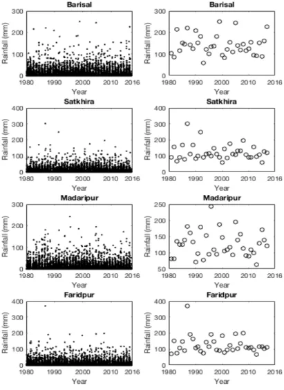
Figure 3: Daily and annual maximum rainfall plots for stations Barisal, Satkhira, Madaripur and Faridpur.

The daily rainfall plot and monthly maximum in Figure 2 shows a clear trend depending on monsoon season. Fig 3 strengthens that it is true for all stations. When studying the annual maximum one can assume that the pattern of variation has stayed constant. This can be checked by analyzing autocorrelation function.

Figure 4: Autocorrelation function for annual maximum rainfall from station Chandpur.

Autocorrelation plots are a tool for checking randomness for time-series data. The x-axis represents the size of the lag between the elements of time-series. The lag 0 is always equal to one because it shows the autocorrelation between itself and each term. The higher value of the spikes the higher autocorrelation for each lag. All spikes that are between the two dashed lines is considered not correlated. The autocorrelation plot for Chandpur is represented in Fig 4. All stations can be assumed to be random time-series according to their autocorrelation plots.

3.2

Block-size selection for GEV

The different blocks were split up into size of one year. Every block maxima represents the highest amount of rainfall during one day for all years between 1980-2016. That is 37 block maxima except for station Chandpur which is missing data from 1980 and leaves us with 36 block maxima. Generalized extreme value distribution was fitted to the block maximas. In order to find out whether GEV was a suitable distribution diagnostic plots was analyzed.

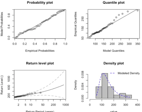
Figure 5: GEV diagnostic for Chandpur with annual maximum block. As can be seen in Figure 5, the points of the probability plot and quantile plot lies close to the unit diagonal. This implies that generalized extreme value distribution function provides a good fit. The return level plot shows that the empirical return levels match well with those from the fitted distri-bution function. Finally, the density plot also shows good agreement between the fitted GEV distribution function and the empirical density.

3.3

Threshold selection for GPD

Thresholds were chosen based on mean residual life plots, threshold range plots and the number of exceeding values. When threshold was chosen diag-nostics plots were analyzed in order to see if GPD was a suitable distribution for the exceeding values. Mean residual life plot, threshold range plots and diagnostic plots for station Chandpur are presented below.

Figure 6: Mean residual life plot for station Chandpur.

Figure 7: Threshold range plot for station Chandpur.

The threshold for Chandpur was chosen at 70. As can be seen in the mean residual life plot there is some evidence for linearity above u = 70. One can also see in the threshold range plot that the selected threshold seems reasonable. For threshold 70 there were 181 exceeding values. Generalized Pareto distribution was fitted to all 181 values.

Figure 8: Threshold u=70 for Chandpur.

Same procedure was made for all of the stations. The threshold selection for each station and the number of exceeding values can be found in Table 1 below.

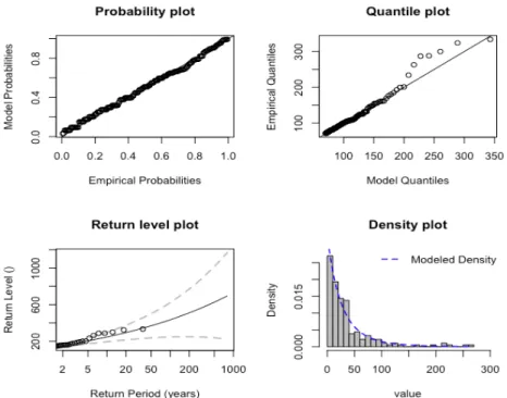
Figure 9: GPD diagnostic for Chandpur with threshold 70 mm.

Just as for GEV distribution diagnostic plots for GPD distribution was made. Figure 8 strengthens that GPD is a reasonable distribution for the exceeding values.

4

Rainfall pattern for the different stations

4.1

Barisal

Barisal is the most southern measure station of all the stations. The maxi-mum rainfall measured at this station was 251 mm which occurred in Novem-ber 1998. The range of annual maximum during the period was [59,251]. The average annual maximum measured at station Barisal during the period 1980-2017 was 142,001 mm. The average annual rainfall was 2086,004 mm per year.

4.2

Chandpur

Chandpur is located in the southern part of Bangladesh and is adjacent to one of the largest rivers, Dakatia, [3]. The maximum rainfall during the measuring period was 334 mm in one day and occurred in June 1983. The lowest annual maximum was 56 mm. The average annual maximum rainfall measured at station Chandpur was 154.582 mm. The average annual rainfall was 2184,103 mm per year which is the highest average annual rainfall of all of the five stations.

4.3

Satkhira

Satkhira station is located in southwestern Bangladesh, near the Indian bor-der. The maximum rainfall measured at this station was 302 mm which occurred in September 1986, the same year and month as Faridpurs maxi-mum rainfall. The lowest annual maximaxi-mum was measured to 58 mm. The average annual maximum measured at station Satkhira during the period 1980-2017 was 122,491 mm, the average annual rainfall was 1710,500 mm per year.

4.4

Madaripur

Faridpur is on the north of Madaripur, Barisal is on the south. The range of annual maximum during the period was [63,243], the highest value occurred

in June 1995. The average annual maximum measured at station Madaripur during the period 1980-2017 was 125,844 mm, the average annual rainfall was 1952,102 mm per year.

4.5

Faridpur

The measure station Faridpur is located in the central part of Bangladesh near the capital Dhaka. The maximum rainfall measured at this station was 370 mm which occurred in September 1986 and the range of annual maximum rainfall during the period was [65,370]. The average annual maximum during the period was 126,572 mm and the average annual rainfall was 1812,181 mm per year.

5

Results

All parameters for GEV distribution an GPD have been estimated and are presented in Table 2 below. Return levels and confidence intervals for both distribution using both delta method and profile likelihood are presented and briefly explained in this section.

5.1

Parameter estimation for extreme rainfall

Maximum likelihood estimation method is used to estimate the parameters of generalized extreme value distribution and generalized Pareto distribution with a 95 % confidence interval. The parameters were estimated using two different methods, delta method and profile likelihood. The two methods gave very similar results for the various confidence intervals. The profile likelihood estimates are presented in the figures and tables below.

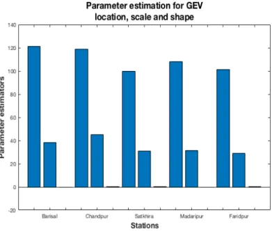
Figure 10: Parameter estimation for GEV distribution. Presented in order location, scale and shape parameters.

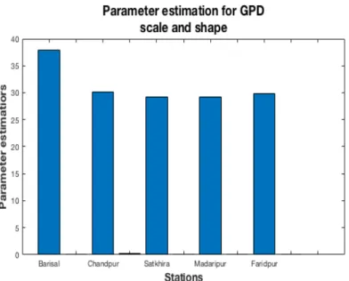
Figure 11: Parameter estimation for GPD. Presented in order scale and shape parameters.

Station Barisal has a negative shape parameter for both GEV distribution and GPD which implies that the distribution belongs to the Weibull family. The confidence interval for station Barisal includes positive values aswell so we can not ignore the fact that it might belong to one of the other families. In the case when the maximum likelihood estimate of shape parameterξ <0 this implies that the support of the GEV distribution is bounden.

The shape parameters of Madaripur are of opposite sign for GEV and GPD. The confidence intervals have values in both domains. Because of this i might belong to the Weibull family but assumptions like that can not be made. Station Chandpur the shape parameter is positive and when looking at the GPD confidence interval all values are positive. This strengthens that it be-longs to the Fr´echet family with no upper end-point.

Faridpur and Satkhira have positive shape parameters but since the con-fidence intervals includes both negative and positive values any assumptions can not be made.

Table 2: Parameter estimation, standard deviation and a 95 % confidence intervals for GEV and GPD using profile likelihood.

5.2

Return level for extreme rainfall

Return levels are the estimates of the extreme quantiles of the distribution during a certain return period, 1_p, in this case either 10, 50 or 100 years. The confidence intervals are calculated with a 95 % significance level. Both delta method and profile likelihood have been used and they are both presented in the two tables below. According to the delta method station Chandpur’s 100 year return level is 282.833 mm for GEV distribution, this means that the expected rainfall 282.833 is to be exceeded on average once every 100 years. The estimates of the return levels are very similar for both GEV distribution and GPD. As can be seen in the tables below the profile likelihood method presents confidence intervals with higher values and over all smaller intervals compared to the delta method. Station Chandpur has significantly higher values compared to the other stations when it comes to both delta method and profile likelihood. Although there is a difference both fits presents return levels that are quite similar. Figure 12 shows that the confidence intervals for the profile likelihood approach are quite asymmetric. The confidence inter-vals implies that the data provides weaker information for the higher return periods.

Figure 12: Profile log-likelihood return level plots for the GEV and GPD fit for station Chandpur.

Table 3: Estimated return levels with a 95% confidence intervals for GEV and GPD using profile likelihood.

Table 4: Estimated return levels with a 95 % confidence intervals for GEV and GPD using the delta method.

5.3

Probable maximum rainfall

Return periods for different years and quantiles are presented in the table below. This method presents significantly higher values compared to block maxima or peaks over threshold method. This might be because this ap-proach is based on significantly more measurements. Even in this method station Chandpur presents the highest predicted future rainfall.

Table 5: Estimated quantiles, probable maximum rainfall, in mm for different risk levels and time periods

6

Conclusions

The aim of this thesis was to make an univariate extreme value analysis to calculate the extreme rainfall pattern over the next 10, 50 and 100 years. Daily rainfall data from five different measuring stations over 37 or 36 years was used. All five stations are geographically close to each other located in the south part of Bangladesh. Since the measurement stations only are located in the southern parts of Bangladesh, we can not comment on the estimated rainfall in other parts of the country.

Trend checks were made and daily rainfall plots shows a clear trend for each station depending on monsoon seasons. Autocorrelations function plots were checked and the data was assumed to be independent. No increase in the amount of rainfall can be seen during the measuring period. The most extreme rainfalls are not from the recent period in particular. All stations were compared to each other and a correlation between all of the stations was shown. Although the dependence is not very strong this indicates that the stations had followed the same rainfall pattern during the measuring period.

First block maxima method was used, the blocks were split up into size of years and generalized extreme values distribution was fitted to the annual maxima. The second method used was peaks over threshold. Thresholds were chosen for the different stations and generalized Pareto distribution was applied to all of the exceeding values. The good fit of the two distribu-tions was checked by diagnostic plots.

All parameters, and their confidence intervals, for both distributions were estimated using two different methods, delta and profile likelihood. Return levels with confidence intervals were also calculated for each distribution using both of these methods. As tables 1-3 show both distributions and methods present very similar values for the parameter estimates and the re-turn levels. This strengthens the assumption that both distributions are a reasonable fit.

The calculated return levels for GEV distribution and GPD does indicate an increase in rainfall for most of the stations. Station Faridpur and station Satkhira have a lower expected maximum rainfall in one day the next 100 years than have already occurred during the measuring period. Although, the probable maximum rainfall method presents higher predicted rainfall the coming 10, 50 and 100 years. According to this model the daily rainfall in one day will increase significantly. This method is considered more reliable because of wider range of observation.

The data was first treated in the program Matlab where all matrices were structured and trend checks were made. All stations were missing data from different days during the measuring period. Very few of these miss-ing measurements were durmiss-ing monsoon period. These missed values may have caused some error margin in the calculations. For peaks over threshold method and probable maximum rainfall method clustering must be taken into consideration. It might be a risk that some of the exceeding values are dependent since some of them might be during a short measuring period. All calculation were made in the program R using the package in2extremes.

7

References

1. Harmeling, Sven. 2008. ’Weather-Related Loss Events And Their Impacts On Countris In 2007 And In A Long-Term Comparison’, Global Climate Risk Index 2009, Germanwatch.

2. Harmeling, Sven and Eckstein, David. 2013. ’Who suffers most from extreme weather events? Weather-related loss events in 2011 and 1992 to 2011’, Global Climate Risk Index 2013, Germanwatch.

3. Mahmood, Shakeel Ahmed Ibne. 2012. ‘Impact of Climate Change in Bangladesh: The Role of Public Administration and Government’s Integrity. Journal of Ecology and the Natural Environment Vol.4(8), 223–240.

4. Rootzen, Holger and Tajvidi, Nader. 1997. Extreme Value Statistics and Wind Storm Losses:A Case Study. Scandinavian Actuarial Journal, 70-94.

5. Ferreira, Ana and De Haan, Laurens. 2014. On the block maxima method in extreme value. University of Lisbon and Erasmus Univ Rotterdam, 1-4. 6. Binte Murxhed, Sonia, Islam, A.K.M Sailful and Alam Khan, M.Shah. 2011. Impact of climate change on rainfall intensity in Bangladesh. 3rd

In-ternational Conference on Water and Flood Managment.

7. Kreft, S¨onke, Eckstein, David and Melchior, Inga . 2017. Global cli-mate risk index 2017: Who Suffers Most From Extreme Weather Events? Weather-related Loss Events in 2015 and 1996 to 2015 Germanwatch

8. The Intergovernmental Panel on Climate Change (IPCC). 2007. Cli-mate change 2007: Impacts, adaptation and vulnerability, Ch:10.

9. Coles, Stuart.2004. An Introduction to Statistical Modeling of Extreme Values. Springer Series in Statistics, Ch: 2-4.

10. S. Cooley, Daniel. 2005. Statistical Analysis of Extremes Motivated by Weather and Climate Studies: Applied and Theoretical Advances. Uni-versity of Colorado at Boulder, 1-7.

11. Plan international. 2017. Life under water: When monsoon season strikes in Bangladesh.

12. Sultana, Nasrin. 2015. A Multivariate Extreme Value Approach to Modeling Risk of Flooding and Drought in Bangladesh. Lund University, Centre for Mathematical Sciences.

13. National Plan for Disaster Management Government of the People’s Republic of Bangladesh 2010-2015. 2010. Government of the People’s Re-public of Bangladesh.

14. Google map. https://www.google.com/maps/place/Bangladesh/ @23.4521973,85.8466443,6z/data=!3m1!4b1!4m5!3m4!1s0x30adaaed80e 18ba7:0xf2d28e0c4e1fc6b!8m2!3d23.684994!4d90.356331, (2018-02-13).