Design and analysis of clustering algorithms for numerical, categorical and mixed data

(1)

Design and Analysis of

Clustering Algorithms for Numerical, Categorical

and Mixed Data

A thesis submitted to Cardiff University

for the degree o f

Doctor of Philosophy

by

Maria Del Mar Suarez Alvarez

Manufacturing Engineering Centre

Cardiff University

(2)

UMI Number: U516748

INFORMATION TO ALL USERS

The quality of this reproduction is dependent upon the quality of the copy submitted.

In the unlikely event that the author did not send a complete manuscript and there are missing pages, these will be noted. Also, if material had to be removed,

a note will indicate the deletion.

Dissertation Publishing

UMI U516748

Published by ProQuest LLC 2013. Copyright in the Dissertation held by the Author. Microform Edition © ProQuest LLC.

ProQuest LLC

789 East Eisenhower Parkway P.O. Box 1346

(3)

ABSTRACT

In recent times, several machine learning techniques have been applied successfully to

discover useful knowledge from data. Cluster analysis that aims at finding similar

subgroups from a large heterogeneous collection o f records, is one o f the most useful

and popular o f the available techniques o f data mining.

The purpose o f this research is to design and analyse clustering algorithms for numerical,

categorical and mixed data sets. Most clustering algorithms are limited to either

numerical or categorical attributes. Datasets with mixed types o f attributes are common

in real life and so to design and analyse clustering algorithms for mixed data sets is quite

timely. Determining the optimal solution to the clustering problem is NP-hard. Therefore,

it is necessary to find solutions that are regarded as “good enough” quickly.

Similarity is a fundamental concept for the definition o f a cluster. It is very common to

calculate the similarity or dissimilarity between two features using a distance measure.

Attributes with large ranges will implicitly assign larger contributions to the metrics than

the application to attributes with small ranges. There are only a few papers especially

devoted to normalisation methods. Usually data is scaled to unit range. This does not

(4)

The first part o f the thesis concentrates on the development o f a mathematically rigorous

approach to normalisation o f the feature vectors for mixed data sets based on a unified

statistical approach. The most common cases o f metrics, namely the Euclidean metrics

are used as a measure for continuous numerical features, while the matching

dissimilarity measure is used to deal with categorical attributes. The introduced

normalised metrics secure that the average contributions o f all attributes to the measures

are equal to each other from statistical point o f view.

The second part o f the thesis concentrates on the application o f the unified statistical

approach to the general case o f the Minkowski metrics and the development o f a novel

algorithm for hard clustering using the Minkowski distances with an appropriate

objective function. The algorithm may be used in these cases, while the k -prototypes is not applicable.

The third part o f the thesis introduces the RANKPRO (the Random Search with k-prototypes algorithm). It combines the advantages o f the B ees and ^-k-prototypes

algorithms and outperforms the latter algorithm. The RANKPRO balances two

objectives: first it explores the search space effectively due to random selection o f new

solutions, and on the other hand it improves promising solutions fast due to employment

(5)

ACKNOWLEDGEMENTS

I would like to thank my supervisor Professor D.T. Pham, for his invaluable guidance

during the course o f this study.

I would also like to thank my family for their love and encouragement.

I am very grateful to Dr. Yuri Prostov for his valuable comments on the thesis and for

discussing the theoretical and practical aspects o f clustering algorithms, related problems

and possible ways to their solution.

I am very grateful to Mr. M. Prostov for his valuable discussions on statistical

approaches to clustering procedures.

I am also grateful to all the members o f the MEC Machine Learning Group for providing

useful technical discussions.

(6)

DECLARATION

This work has not previously been accepted in substance for any degree and is not being

concurrently submitted in candidature for any degree.

Signed... (Maria del Mar Suarez Alvarez - Candidate)

Date . 2 . 0 0 % ...

Statement 1

This thesis is being submitted in partial fulfilment o f the requirements for the degree o f

Doctor o f Philosophy (PhD).

Signed (Maria del Mar Suarez Alvarez - Candidate)

D ate... . . . . S s p ...

Statement 2

This thesis is the result o f my own independent work/investigation, except where

otherwise stated. Other sources are acknowledged by explicit references.

Signed f i . . (Maria del Mar Suarez Alvarez- Candidate)

(7)

Statement 3

I hereby give consent for my thesis, if accepted, to be available for photocopying and for

inter-library loan, and for the title and summary to be made available to outside

organisations.

Signed /.7...<7VT7...(Maria del Mar Suarez Alvarez - Candidate)

(8)

CHAPTER 3 CLUSTERING MIXED DATA SETS (EUCLIDEAN

METRIC) BY USING THE X-PROTOTYPES ALGORITHM

50

3.1 Background 51

3.2 Some specific features o f the k -means algorithm 54

3.3 Normalisation o f feature vectors 57

3.3.1 Normalisation o f numerical data sets 58

3.3.2 Normalisation o f categorical data sets 61

3.4 Statistical approach to normalisation o f feature vectors 62

3.4.1 Estimators 62

3.4.2 Earlier attempts o f normalisation 64

3.4.3 A new statistical approach to normalisation o f attributes 66

3.4.4 Data sets with mixed attributes 68

3.5 Comparing the accuracy o f the clustering algorithms 71

3.5.1 Accuracy o f clustering and Rand index 71

3.5.2 Assignment problem and calculating the accuracy o f clustering 73

3.6 Applications to data sets 85

3.6.1 Soybean Disease Data Set 85

3.6.2 Wine Data Set 91

3.6.3 Statlog (Heart Diseases) Data Set 96

3.6.4 Credit Approval Data Set 102

(11)

CHAPTER 4 CLUSTERING MIXED DATA SETS (MINKOWSKI

METRIC)

110

4.1 Background 110

4.2 Statistical approach to normalisation o f the Minkowski metric (numerical

attributes) 112

4.3 Normalisation o f metrics for data sets with mixed attributes 115

4.4 A general algorithm for normalisation o f mixed metrics 118

4.5 Clustering algorithms based on Minkowski metrics 119

4.5.1 Algorithm 119

4.5.2 Clustering using Minkowski metrics 119

4.6 Applications o f the algorithms based on Minkowski metrics to data sets 125

4.6.1 Adult data set 125

4.6.2 Shuttle data set 128

4.7 Summary 131

C H A P T E R 5 IM P R O V IN G THE K -P R O T O T Y P E S A LG O R IT H M

BY R A N D O M SE A R C H

133

5.1 Background 134

5.2. Preliminaries 135

5.2.1 The A:-means and A:-prototypes algorithms 135

(12)

5.3 Description o f RANKPRO 142

5.3.1 Normalisation o f metrics for mixed data sets 142

5.3.2 Pseudo code o f RANKPRO 144

5.4 Applications to data sets 146

5.4.1 Comparing the effectiveness o f the clustering algorithms 146

5.4.2 Adult data set 148

5.4.3 Shuttle data set 154

5.4.4 Covertype data set 160

5.4.5 C onnect-4 data set 164

5.5 Summary 167

C H A PT E R 6 C O N C L U SIO N S AN D FU TU R E W O R K

169

6.1 Contributions 169

6.2. Conclusions 170

6.3. Future Research Directions 171

R E FE R E N C E S

173

A P P E N D IC E S

192

A PPE N D IX A

D ataSets 192

A PPE N D IX B

Proof o f unbiasedness and consistency o f estimators used for

(13)

LIST OF FIGURES

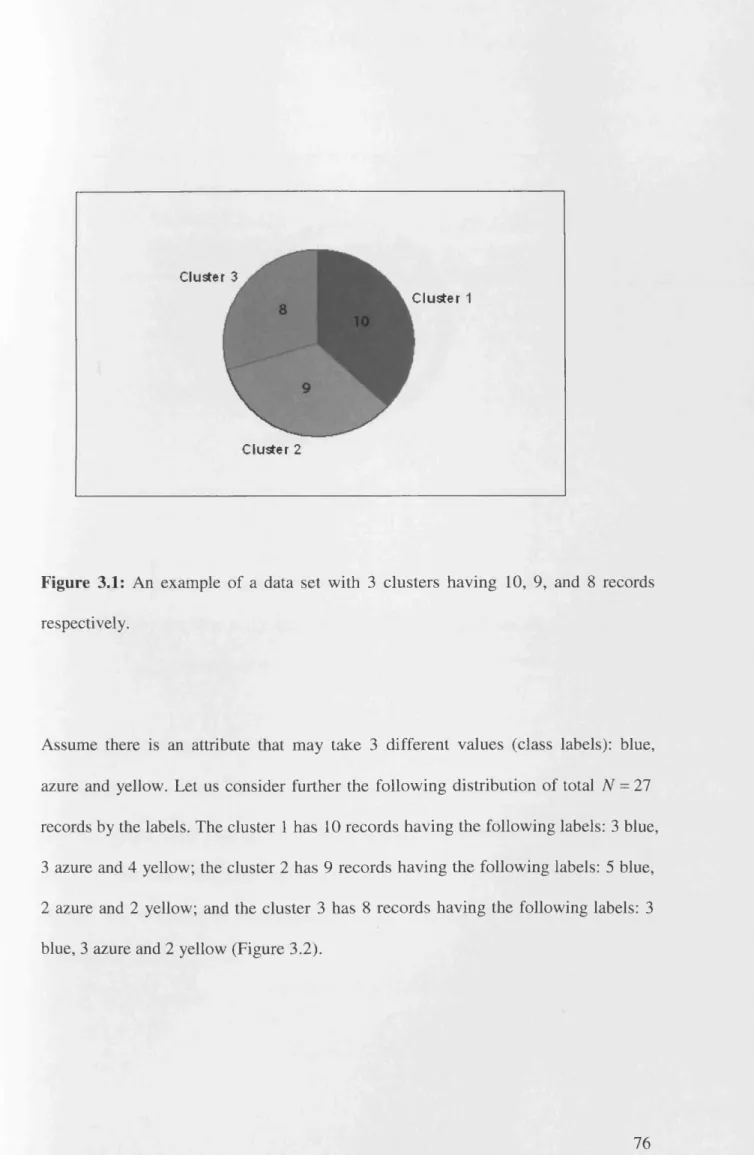
Figure 3.1: An example o f a data set with 3 clusters having 10, 9, and 8 records

respectively. 76

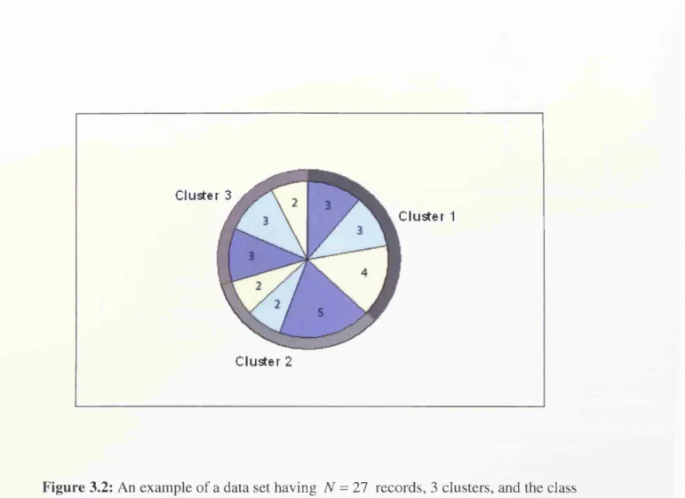
Figure 3.2: An example o f a data set having N = 27 records, 3 clusters, and the class labels o f the records: blue, azure and yellow. The cluster labels are not yet assigned. 77

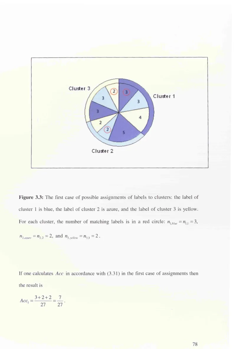
Figure 3.3: The first case o f possible assignments o f labels to clusters: the label o f

cluster 1 is blue, the label o f cluster 2 is azure, and the label o f cluster 3 is yellow. For

each cluster, the number o f matching labels is in a red circle: blue = n lx = 3,

n i , ^ r e = «2,2 = 2. a n d = « 3 .3 = 2

78

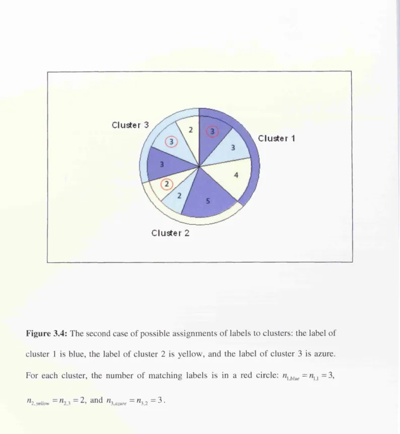
Figure 3.4: The second case o f possible assignments o f labels to clusters: the label o f

cluster 1 is blue, the label o f cluster 2 is yellow, and the label o f cluster 3 is azure. For

each cluster, the number o f matching labels is in a red circle: nxblue= n xx = 3,

n 2,yellow = W2,3 = a i ^ ^ 3 , azure = W3,2 = ^ • ^ 9

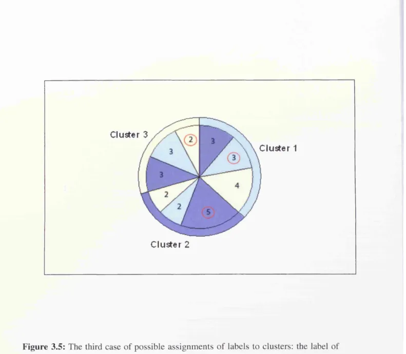
Figure 3.5: The third case o f possible assignments o f labels to clusters: the label o f

cluster 1 is azure, the label o f cluster 2 is blue, and the label o f cluster 3 is yellow. For

each cluster, the number o f matching labels is in a red circle: nx azure =nx 2 = 3,

(14)

each cluster, the number o f matching labels is in a red circle: azure = nx 2 = 3,

n2,yellow = W2,3 = 2’ and n3,blue = W3,l = 3 ' 8 ^

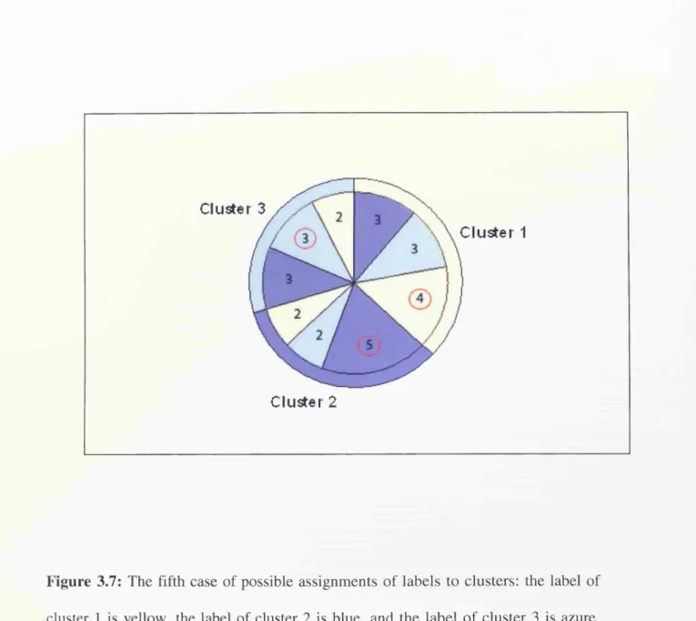
Figure 3.7: The fifth case o f possible assignments o f labels to clusters: the label o f

cluster 1 is yellow, the label o f cluster 2 is blue, and the label o f cluster 3 is azure. For

each cluster, the number o f matching labels is in a red circle: nlyellow = nl3 = 4,

n2,blue = n2,\ ~ and n3 azure — n3 2 — 3 • 82

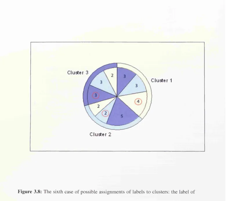
Figure 3.8: The sixth case o f possible assignments o f labels to clusters: the label o f

cluster 1 is yellow, the label o f cluster 2 is azure, and the label o f cluster 3 is blue. For

each cluster, the number o f matching labels is in a red circle: nx llaw = nx 3 = 4,

^2,azure= W2.2 = 2 > » n d « 3,blue = W3,l = 3 • 8 3 Figure 5.1: The average values o f ^ ( S ) vs. taec for the Adult data set with fixed

parameters n , e and r (e = l) . Comparison o f the k -prototypes algorithm and the

RANKPRO algorithm 150

Figure 5.2: The average values o f ./av(S ) vs. for the Adult data set for (e = l) and

(e = 2 ). Comparison o f the k -prototypes algorithm and the RANKPRO algorithm 151

Figure 5.3: The average values o f ^av(S ) vs. for the Adult data set with fixed

parameters n , e and r (e = 2) . Comparison o f the k -prototypes algorithm and the

Figure 5.4: The average values o f Jav(S )v s . tmc for the Adult data set with fixed

parameters niter and e. Comparison o f the k -prototypes algorithm and the RANKPRO

(15)

Figure 5.5: The average values o f ^av(S ) vs. for the Shuttle data set with fixed

parameters n , e and r (e = l) . Comparison o f the k -prototypes algorithm and the

Figure 5.6: The average values o f J flV(S )v s. for the Shuttle data set for ( e - 1) and

(e = 2 ). Comparison o f the k -prototypes algorithm and the RANKPRO algorithm 157

Figure 5.7: The average values o f J av (S ) vs. taec for the Shuttle data set with fixed

parameters n, e and r (e = 2 ) . Comparison o f the k -prototypes algorithm and the

RANKPRO algorithm 15 8

Figure 5.8: The average values o f Jrav(S )v s. for the Shuttle data set with fixed

parameters niter and e. Comparison o f the k -prototypes algorithm and the RANKPRO

algorithm 159

Figure 5.9: The average values o f ^ ( S ) vs. for the Covertype data set with fixed

parameters n , e and r (e = l) . Comparison o f the k -prototypes algorithm and the

Figure 5.10: The average values o f J av (S ) vs. for the Covertype data set for ( e = l)

and (e = 2 ). Comparison o f the k -prototypes algorithm and the RANKPRO algorithm

162

Figure 5.11: The average values o f J av(S )v s. for the Covertype data set with fixed

parameters n , e and r (e = 2) . Comparison o f the k -prototypes algorithm and the

(16)

Figure 5.12: The average values o f J av (S ) vs. for the Connect-4 data set with fixed

parameters n , e and r (e = l) . Comparison o f the k -prototypes algorithm and the

Figure B . l : Sets Vx and V2 for N = 7 : a) the set Vx and b) the set V2 199

(17)

LIST OF TABLES

Table 2.1: A modified Stevens’ classification o f variables (scale types), and appropriate

statistical notions, mathematical operations and structure. 12

Table 3.1: Clustering o f the soybean data set without normalisation o f the attributes. 86

Table 3.2: Clustering o f the soybean data set with normalisation o f the attributes. 88

Table 3.3: Clustering o f the wine data set without normalisation o f the attributes. 91

Table 3.4: Clustering o f the wine data set with normalisation o f the attributes. 94

Table 3.5: Clustering o f the heart diseases data set without normalisation o f the

attributes. 97

Table 3.6: Clustering o f the heart diseases data set with normalisation o f the attributes.

99

Table 3.7: Clustering o f the credit approval data set without normalisation. 102

Table 3.8: Clustering o f the credit approval data set with normalisation. 105

Table 4.1: Clustering o f the Adult data set without normalisation o f attributes for various

values o f the Minkowski power p M 126

Table 4.2: Clustering o f the Adult data set with normalisation o f attributes for various

values o f the Minkowski power p M 127

Table 4.3: Clustering o f the Shuttle data set without normalisation o f attributes for

various values o f the Minkowski power p M 129

Table 4.4: Clustering o f the Shuttle data set with normalisation o f attributes for various

(18)

ABBREVIATIONS

BA Bees Algorithm.

CRS Controlled Random Search.

EM Expectation Maximisation Algorithm.

GA Genetic Algorithms.

LBS Local beam search.

OF-based clustering Objective function-based clustering.

RANKPRO The Random Search with k -Prototypes Algorithm.

SBS Stochastic beam search.

(19)

SYMBOLS

A, Records o f a data set.

X ,, Numerical part o f a record o f a data set.

Y ., Categorical part o f a record o f a data

set.

XXj, X 2j Independent random variables.

N Number o f records in a data set or the number o f elements in a sample.

p Number o f numerical attributes in a record.

/ Number o f categorical attributes in a record.

Lp Linear vector space (Minkowski space).

p E Euclidean metric.

p cat Categorical metric.

p max Tchebysheff (Chebyshev) or maximum norm metric.

p* Normalised Minkowski metric.

^ Pm

p H Huang’s mixed metric.

y Weight in the Huang mixed metric.

J Objective function.

J . Hathaway’s objective function.

uim Element o f the partition matrix.

(20)

Q m Prototype (centre).

C _tn Cluster m .

IC I Number o f elements in the cluster C„ .

| m | m

X = ( X v X 2i..., X N) Random vector formed by a sequence o f random variables,

x

= (x,, x2 ) The actually observed sample value.

x*j Normalised attribute value in the data set.

x_{m a x j} Maximum value o f an attribute.

x_{m m j} Minimum value o f an attribute.

Hj and crj Mean and standard deviation o f a random variable.

X j and Sj Estimators for mean and standard deviation o f a sample.

dj(X'j, xfj) Hastie’s attribute dissimilarity.

Z)(jc, , xf) Hastie’s overall measure o f dissimilarity.

Wj Weight assigned to the j -th attribute.

D Hastie’s average object dissimilarity measure.

dj Hastie’s average dissimilarity o f the y'-th

attribute.

E Expectation o f a variable.

E Estimator o f the expectation.

s 2. Estimator o f the sample variance.

(21)

a. Inverse o f expectation o f contribution o f the j -th numerical attribute to a

metric.

Pj Inverse o f expectation o f contribution o f the j -th categorical attribute to a metric.

{ p j v p n , . . . , p , qi}

attribute.

A ccs,w

C = {C i,...,C 4} , D = {2>„... , Dt ]

R

Probabilities o f possible states for a categorical

Distance between two categorical attributes.

The N g and Wong accuracy.

Two partitions o f a set.

the Rand index.

m , j Number o f records with the attribute that belongs to the m -th cluster.

n , v Number o f records o f the m -th cluster whose state o f the attribute A is the same

as the assigned av{m)

Acc{(p) Acc T{x) X ' Pm (p(zv z 2) D

Clustering accuracy for an assignment (p.

Clustering accuracy.

Euler gamma function.

Minkowski norm.

Function o f two real valued arguments (Proposition 4).

Sets o f chords used in the proof o f Lemma 4.

Dispersion.

Subgradient o f 0 .(0*

(22)

Number o f best sites (BA).

Number o f elite sites (BA).

Size o f neighbourhood around any o f the best sites (BA).

Number o f recruited bees within the neighbourhood for the elite sites (BA).

Number o f recruited bees around other selected sites (BA).

Number o f the approximate solutions (RANKPRO).

Number o f kept elite solutions (RANKPRO).

Number o f solutions used for random search (RANKPRO).

Time specified for the RANKPRO algorithm.

Given number o f simulations for the RANKPRO algorithm.

Average value o f the objective function obtained in nr simulations.

(23)

Chapter 1

Introduction

This chapter introduces the motivation and objectives o f the research, and a general

description o f adopted methods and approaches. The chapter also outlines the general

structure o f the thesis.

1.1 Motivation

There is an increasing amount o f data being collected everyday but only the part that can

be used for extracting knowledge becomes valuable. Data Mining (DM ) may be defined

as a process o f extracting useful knowledge in the form o f relations and structure from

large amount o f data. The derived knowledge can then be applied to achieve economic,

operational or other benefits.

In this thesis DM is considered as a synonym to the knowledge discovery process or

knowledge discovery in databases. This process consists o f a set o f processing steps that

should be followed to discover relations and structure in data. DM needs to develop

(24)

from raw collections o f data. In this thesis we deal with objective function-based

clustering that is also called partition based clustering.

Partitioning is a natural way o f studying complex problems in a number o f areas like

pattern recognition, classification and clustering. In a number o f fields o f machine

intelligence, an object is represented by a vector variable (the feature vector). In

application to data sets organised as flat files, the rows represent records, the columns

represent features that are called attributes, and hence the feature vector can be defined

as a set o f attributes. Each attribute can take on a finite or infinite (continuous) number

o f possible values. In many traditional applications, it is assumed usually that all the

features are the same type. Clustering o f numerical data sets are the most studied

problem. However, real-life data sets are often mixed, i.e. they consist o f both numerical

and categorical types. Currently methods for analysis o f data in mixed feature space are

still an issue. Hence, design and analysis o f clustering algorithms for numerical,

categorical and mixed data sets are very timely.

In this thesis we w ill deal with normalisation. Strictly speaking normalisation has to be

applied to all records o f data sets before clustering. Indeed, if the data is not normalised

then the average contribution o f each feature to the similarity measure depends on the

units o f measurements o f the feature and, therefore, the contribution o f the features are

scale dependent. If the units o f a measurement are changed then the contribution o f a

feature to the similarity measure can change dramatically. This is why normalisation o f

data sets is widely used in a number o f fields o f machine intelligence.

(25)

In the overwhelming majority o f published normalisation procedures, data have been

scaled to unit range. However, after this kind o f data set normalisation, the average

contributions o f all features to the similarity measure may be not equal to each other.

It has been often suggested also to truncate the out-of-range components assuming that it

is just eliminating the outliers. However, truncating the out-of-range components could

lead to loss o f information from the data set.

In spite o f the importance o f data normalisation, there have been only few papers

specifically devoted to normalisation methods for data sets. It has been correctly realised

that a normalisation procedure for numerical data sets, has to be a transformation o f the

attribute to a random variable with zero mean and unit variance. Indeed, this scaling

provides equal contributions o f variables to the Euclidean similarity measure. However,

one needs to apply normalisation not only to numerical attributes but also to categorical

attributes.

A natural way for normalisation o f all numerical, categorical and mixed data sets is to employ a statistical approach. However, early papers on statistical approaches were not

targeted to clustering o f mixed data sets and normalisation o f metrics. It was stated that

methods for analysis o f data in mixed feature space are still an issue. For example, one

can expect that the mean o f the distance between two categorical attributes that may

have only two states (e.g. male - female or white - black) is not the same as the mean o f

the distance between two categorical attributes that may have twenty different states.

(26)

nothing was known about statistical consistency o f the proposed estimators. In addition,

the estimators were biased and these approaches were not applicable to some metrics.

Hence, mathematically rigorous treatment o f the normalisation procedure is needed and

explicit presentation o f normalised mixed metrics has to be provided.

After normalisation o f data, appropriate algorithms for efficient and effective clustering

o f data sets with mixed numerical and categorical values have to be developed. Currently

the most popular is the ^-prototypes algorithm for clustering o f mixed data sets. This

algorithm is a generalisation o f the A:-means algorithm. The latter is applicable only to

numerical data sets. These algorithms have the same common drawback, namely the

search process o f new solutions converges often not to a global minimum but to a local

minimum. Hence, new algorithms have to balance two objectives: to explore the search

space effectively and to utilise the most promising solutions during the work o f the

algorithm.

1.2 Research Objectives

The aim o f this research is to design and analyse new clustering algorithms for numerical,

categorical and mixed data sets. Most clustering algorithms are limited to either

numerical or categorical attributes. Datasets with mixed types o f attributes are common

in real life and so to design and analyse clustering algorithms for mixed data sets is quite

timely.

(27)

The specific objectives are:

1. To develop a mathematically rigorous approach to normalisation o f feature

vectors for mixed data sets based on a unified statistical approach.

2. To analyse the clustering algorithms with proposed new normalised metrics in

the case o f the matching dissimilarity measure being used to deal with categorical

attributes, and the general Minkowski metrics being used as a measure for

continuous numerical features, including the particular cases p M = 2 (the

Euclidean metric).

3. To develop a new algorithm to be used in the cases where p M * 2 , since the k

-prototypes cannot be used in those cases. This clustering algorithm was earlier

suggested only for fuzzy clustering. It will be developed and applied for hard

clustering using Minkowski norm distances.

4. To develop a new unsupervised clustering algorithm for numerical, categorical

and mixed data sets that will have less probability for premature convergence

than the ^-prototypes algorithm. The algorithm has to balance two objectives: to

explore the whole search space effectively, and to improve promising solutions

fast. The new algorithm has to combine the advantages o f both the Bees and the

(28)

1.3 Methods and approaches

For the four objectives targeted in this thesis, several methods and approaches will be

employed. They are summarised as follows:

1. A unified statistical approach to both numerical and categorical attributes is

applied for normalisation o f the feature vectors for mixed data sets in both

cases; the Euclidean and the general Minkowski metrics. Normalised

Minkowski and Euclidean metrics and metrics for mixed data sets are

introduced in an explicit way. The introduced generalised statistical

procedure assures that the means o f the different normalised attributes are

equal to each other and therefore, these variables give equal contributions to

the similarity measures.

2. In the case where p M = 2 , the ^-prototypes clustering algorithm will be implemented and applied to data sets from the UCI repository with and

without normalisation o f attributes and the accuracy o f clustering results will

be compared by both a new approach for calculating the accuracy and the

traditional Rand index.

3. A unified statistical approach to general cases o f the Minkowski distances

and the development o f a novel algorithm for hard clustering using the

Minkowski distances with an appropriate objective function. Implemented

(29)

codes are applied to two data sets from the UCI repository with and without

normalisation o f attributes for various values o f the Minkowski power p M .

4. A new clustering algorithm called RANKPRO: the Random Search with k-prototypes algorithm will be presented. The algorithm combines the

advantages o f the Bees and ^-prototypes algorithms. The algorithm balances

two objectives: it explores the search space effectively due to random

selection o f new solutions, and improves promising solutions fast due to

employment o f the ^-prototypes algorithm. The RANKPRO algorithm will be

applied to various data sets, including data sets with mixed numerical and

categorical values and its performance w ill be compared with the

performance o f the ^-prototypes algorithm.

1.4 Outline of the thesis

The thesis is organised in six chapters. The topics addressed in each chapter are as

follows:

Chapter 2: In this Chapter notations and definitions o f some concepts related to

clustering, similarity measures for numerical, categorical and mixed data sets, objective

functions, and statistical estimators, are recalled. The chapter ends with a literature

review o f the most recent applications o f object-function based clustering for mixed data

(30)

Chapter 3: In this Chapter a unified statistical approach to both numerical and

categorical attributes is applied in order to normalise the feature vectors for mixed data

sets. The most common cases o f metrics, namely the Euclidean metrics are used as a

measure for continuous numerical features, while the matching dissimilarity measure is

used to deal with categorical attributes. N ew normalised metrics are introduced such that

the average contributions o f all attributes to the measures are equal to each other from

statistical point o f view. Advantages o f the introduced normalised metrics are

demonstrated on examples o f their applications to various data sets.

Chapter 4: In this chapter, a new statistical approach introduced in Chapter 3 is

developed further and applied in the case o f the Minkowski metrics being used as a

measure for continuous numerical features, while to deal with categorical attributes

again the matching dissimilarity measure is used. Various mathematical problems related

to the normalisation o f mixed metrics are resolved. The introduced metrics are applied to

some data sets when it is more advantageous to apply the general Minkowski metrics

(including the Tchebysheff and city-block metrics) instead o f a particular case p M = 2

(the Euclidean metrics). Since the k -prototypes cannot be used in the cases where p M * 2 , a new algorithm to be used in those cases w ill be developed. This clustering algorithm was earlier suggested only for fuzzy clustering. It will be developed

and applied for hard clustering using Minkowski norm distances.

Chapter 5: In this Chapter a new clustering algorithm called RANKPRO: the Random

Search with ^-Prototypes Algorithm is presented. The algorithm combines the

(31)

advantages o f a recently introduced by Pham et al. (2006b) population-based search

algorithm called the Bees Algorithm (BA), and ^-prototypes algorithm proposed by

Huang (1997b) as an extension o f the &-means algorithms to cluster large data sets with

mixed numerical and categorical values. The RANKPRO algorithm balances two

objectives: it explores the search space effectively due to random selection o f new

solutions, and improves promising solutions fast due to employment o f the ^-prototypes

algorithm. The efficiency o f the new algorithm is demonstrated by clustering several

numerical, categorical and mixed data sets.

Chapter 6: In this Chapter conclusions and the main contributions o f this thesis are

(32)

Chapter 2

Preliminaries and Literature Review

In this Chapter notations and definitions o f some concepts related to data models,

clustering, similarity measures for numerical, categorical and mixed data sets, and

objective functions, are recalled. Some mathematical and statistical notions used in

clustering analysis are also reminded. The chapter ends with a literature review o f the

most recent applications o f objective - function based clustering for mixed data sets.

2.1 Data and data types

It is well known (see e.g. Jain and Dubes, 1988, Cios et al., 2007) that data can have

diverse formats and can be stored trough a variety o f different storage models. In a

number o f fields o f data mining an object is represented by a vector variable, namely the

feature vector A (Jain et al. 1999). In application to databases, the features are called

attributes, and hence A can be defined as a set o f attributes A = [Av A2,...,Ap+l} . The

collection o f objects described by the same features is called a data set. Data sets may be

stored as flat files and in other formats using databases and data warehouses. Flat

(rectangular) files are the most common way to store the data sets and further we will

deal only with flat files. The rows represent objects (also known as records, individuals,

patterns, data points) and the columns represent features.

(33)

Each attribute can take on a finite or infinite (continuous) number o f possible values. In

many traditional applications, it is assumed usually that all the features are the same type.

However, real-life data sets are often mixed, i.e. they consist o f both numerical and

categorical types. It is known that the measurement scale o f a categorical variable

consists o f a set o f categories. Only two data types o f attributes are considered here,

namely numerical and categorical because other types o f attributes can be transformed to

these two types. For mixed data, the vector o f features A can be split into A = ( A ”, A c ) ,

namely the vector o f numerical features A" = ( A " , . . . , Aand the vector o f categorical

features A c = ( A tc,..., A f ) .

2.1.1 Original Stevens’ classification of variables.

It is generally accepted that the "levels o f measurement", or scales o f measure are

expressions that typically refer to the classification o f scale types developed by the

psychologist S.S. Stevens. Stevens (1946) argued that measurements can be classified

into four different types o f scales: nominal, ordinal, interval and ratio.

Stevens’s classification said that nominal is synonym o f categorical. There has been, and

continues to be, debate about the merits o f Stevens’s classification, particularly in the

(34)

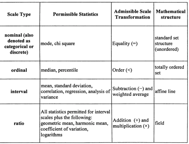
The Table 2.1 presents a slightly modified classification o f variables and appropriate

statistical notions and mathematical operations that should be used for analysis o f each

scale type o f variables

Scale Type Perm issible Statistics A dm issible Scale

T ransform ation M athem atical structure nominal (also denoted as categorical or discrete)

mode, chi square Equality (=)

standard set structure (unordered)

ordinal median, percentile Order (<) totally ordered

set

interval

mean, standard deviation,

correlation, regression, analysis o f variance

Subtraction ( - ) and

weighted average affine line

ratio

A ll statistics permitted for interval scales plus the following:

geometric mean, harmonic mean, coefficient o f variation,

logarithms

Addition (+) and multiplication (x) field

Table 2.1: A modified Stevens’ classification o f variables (scale types), and appropriate

statistical notions, mathematical operations and structure.

(35)

2.1.2 Accepted classification of variables.

In this thesis w e accept the term categorical as a general term that can be split into

levels: nominal and ordinal. If categorical variables have ordered scales they are called

ordinal variables, while the variables having no ordered scales are called nominal

variables. Hence, for nominal variables, the order o f listing the categories is irrelevant,

and the statistical analysis should not depend on that ordering (Agresti 1996). We

consider also binary variables as categorical.

Further, in this thesis we accept the scale types: interval and ratio are numerical variables.

For numerical or quantitative features, the feature domain D om (A y ) can be represented

on the real line, i.e. they are continuous variables. For categorical features (sometimes

these features are also called qualitative), the domain is a finite set o f different states.

Evidently, categorical features may be represented by numerical codes o f possible

different states o f the feature. A data set can be represented as a matrix o f size

N x ( p + l) where N is the number o f records, and ( p + l) is the total number o f attributes, i.e. the i -th row o f the matrix represents the i -th record o f the data set ( \ < i < N ) . This row is a vector (xn, . .., xip, y n,.. ., y a ) , whose values xip are

numerical, while the values y n ,^>,ya are categorical.

One can see from the above Table that the central tendency o f a categorical attribute can

(36)

by Huang (1997, 1998) in his generalisation o f a very popular clustering algorithm, the

&-means algorithm. If the k -means algorithm can be applied only to numerical data sets, the k -modes algorithm can be applied to categorical data sets. These algorithms will be discussed later.

2.2 Constructing data models

As it has been noted in Chapter 1, the aim o f Data Mining is to extract knowledge from

data. Methods o f machine analysis o f data can be roughly divided into two fundamental

groups: supervised and unsupervised learning.

In supervised learning, characteristics to records o f data sets are given. The

characteristics can be expressed either in the form o f some discrete labels or as some

values o f auxiliary continuous variables. In the former case, w e deal with a classification

problem; while in the later case we deal with a regression, or an approximation, or

continuous prediction problem (see e.g. Cios et al., 2007). Supervised learning includes

various approaches such as statistical methods, including Bayesian methods (Pham and

Ruz, 2009); neural networks; decision trees, rule algorithms, and their hybrids. Any

supervised learning method has to be provided with a training data set that represents

information about some domain o f the data set. In classification problems, the objective

o f supervised learning is to construct a function (classifier) that generates for each record

(individual) a class label as its output. Using a training data set rules are produced; these

(37)

rules are used to predict the labels o f new unseen examples (i.e., examples not in the

training set).

Unsupervised learning assumes that the data knowledge process does not involve any

supervision and it discovers a structure in data automatically. Unsupervised learning

includes various approaches such as association rules and clustering. Clustering aims at

finding smaller, more homogeneous groups from a large heterogeneous collection o f

items (Anderberg, 1973, Berry and Linoff, 1997). Computer-assisted analysis must

partition objects into groups, and must provide an interpretation o f this partition (Berry

and Linoff, 1997).

As it is well known, clustering is an inductive process (Bezdek and Pal, 1992, Estivill-

Castro, 2002). This means that using particular observations o f data, isolated facts are

explained first by some empirical generalisations (working hypotheses) and then by a

general theory. In application to clustering o f data sets, this means that any partition

produced by an algorithm or a human is a hypothesis to suggest (or explain) groupings in

the data. The mathematical formulation o f the inductive principle is called clustering

criterion (see e.g. Kim et al., 1988; Doherty et al., 1988, Estivill-Castro and Murray,

1998, Halkidi et al., 2000; 2001). It discriminates one grouping hypothesis over another

one for the same data set. The models are the structures used to represent clusters, while

the induction principle selects a “best fit” model for a given data set. Several induction

(38)

By breaking the object into smaller homogeneous parts that can be each analysed and

explained separately, one can understand very sophisticated phenomena. The selected

hypothesis becomes a model for the data, and can potentially constitute a mechanism to

classify unseen instances o f the data. This is the reason why clustering algorithms have

been studied so extensively. In particular, efficient clustering is a fundamental task in

data science, where the goal is to discover similarities within a large data set.

2.3 Some mathematical notions used in clustering

analysis

The cluster analysis in general and the objective function-based cluster analysis in

particular are mathematically based disciplines where one needs to work with various

mathematical notions like norm, metric, distance, and others. Hence the definitions of

these mathematical concepts and the proper use o f the concepts are crucial for cluster

analysis. Indeed, the aim o f clustering is to group the closest data points together. Hence,

clustering relays on calculating distances between records. Thus, to measure

quantitatively the distinction between elements o f the data sets, i.e. to formulate

similarity or dissimilarity criteria, one needs to use the concept o f the distance and other

above mentioned concepts.

(39)

2.3.1 Concepts of metric and distance.

Let us consider a set M . A metric on a set M is a function which defines a positive real number (distance) between any two elements x and y o f the set. For all x, y , z in M , a metric should satisfy the following conditions:

Identity o f indiscemibles: p ( x , y ) - 0 if and only if x = y .

Non-negativity: p ( x , y ) > 0 .

Symmetry: p ( x , y ) = p ( y , x) .

The triangle inequality: p ( x , z ) < p ( x , y ) + p ( y , z ) .

An example o f a trivial metric is the discrete metric, i.e. if x = y then p ( x , y ) = 0.

Otherwise, p ( x , y ) = l . However, the most popular example is the Euclidean distance;

the distance between distinct points is positive and the distance from x to y is the same

as the distance from y to x. The latter metric is translation and rotation invariant.

Other examples o f metrics w ill be given later. We will consider mainly Minkowski

(40)

2.3.2 Concept of norm.

Let us consider a real vector space/?”, i.e. its elements x e Rnare vectors with real valued entries. A norm o f a vector x is denoted by||jc||. This is a function that assigns a

strictly positive real number to all vectors in the vector space, other than the zero vector.

A norm should satisfy the following conditions:

1

. ||

a

'||

> 0 if x * 0 ,and ||x|| = 0 if and only if x = 0 .

2. A norm is a linear function, i.e. multiplying a vector by a real number a changes its norm linearly

IMbM-M-3. A norm satisfies the triangle inequality for any two elements x and y .

In the case o f norm beign a distance, this inequality means that the distance from point A

through B to C is never shorter than going directly from A to C.

The above mentioned definitions allow the researcher to dismiss some models suggested

for clustering. For example, Wu and Yang (2002) introduced an alternative to c-means

clustering algorithm and they employed the following function:

d ( x , y ) = 1 - exp(-/?||x - y f ) .

(41)

They called this function “distance” and claimed that it is a metric. However, one can

see that d does not satisfy the triangle inequality and therefore this function is not a metric.

There is the following relation between norms and metrics:

Every norm determines a metric and some metrics determine a norm.

Norms are used in Chapters 3 and 4.

2.3.3 Concepts of random variables, mathematical expectation, mean,

mode and median.

Throughout this thesis w e will employ statistical treatment o f data sets. In the framework

o f our approach each record (the row) o f a data set w ill be regarded as a random sample

o f a population under consideration, i.e. a data set is treated as a set o f N observations (samples), while each sample (record) is considered as a realisation o f possible values o f

the feature vector A . O f course, the basic concepts can be found elsewhere (see, e.g.

Spiegel, 1975). Hence, only some concepts o f probability theory and statistics that will

be actively used in the thesis will be recalled. As usual, capital letters X and Y will be used to denote random variables and lower-case letters, x and y to denote the specific values that those variables may take.

(42)

For a continuous random variable X that has a density function / (x) , the mathematical expectation o f E ( X) is defined as

oo

E ( X ) = J x f ( x ) d x . —oo

Another term for the mathematical expectation is the mean that is denoted by jux or by

H. It represents the average o f the values o f the random variable.

The median o f the random variable X corresponds to an ordinate which separates the area under the density function graph into two parts having equal areas, i.e. the median is

that value x for which

P ( X < x ) = J > ( X> x ) =

The mode is that value x which occurs most often or, in other words, has the greatest probability o f occurring. At this value / (jc) has its maximum.

2.3.4 Concepts of statistic and estimators.

For statistical treatment o f feature vectors, one needs to know the probability

distributions o f their attributes. Probability distributions are normally unknown because

one has only a random sample. It is known that estimation is a way o f extracting

valuable information about the distribution o f probability that generated it from a sample.

(43)

An observable function o f the random data variable is called a statistic. If there is an

unknown real parameter 6 taking values in a real parameter space then a real-valued statistic that is used to estimate the parameter is called an estimator o f this parameter. An

estimator can be treated as a guess o f the true value Qtr o f the parameter 6. It is expected

that estimates are close to the true value 0tr. However, since an estimator is a random

variable and it is characterised itself by its probability distribution, one cannot say with

certainty that an estimate is close to the true value o f a parameter o f the distribution. It is

only possible to hope that the central region o f the distribution o f the estimator is close to

the true value o f the parameter. To express this hope in a mathematical way, the concept

o f unbiased estimators is introduced. The properties o f estimators w ill be considered

below.

2.3.5 Desirable properties of estimators.

For any given parameter, different estimators are possible. Hence, it is generally

accepted that estimators have to satisfy the following main desirable properties: an

estimator has to be unbiased, consistent and efficient.

Let us consider a statistic o f size N . An estimator is said to be unbiased if E[0]n = 0tr for any size N .

(44)

Here E means the expectation o f a variable. Roughly speaking, the above definition means that the distribution mean o f the estimator is equal to the true value o f the

parameter for any size o f the statistic. An estimator whose expectation is not equal to the

true value is said to be biased.

An estimator is a consistent estimator o f the parameter, if as sample size increases, the

estimator gets closer and closer to the value o f the parameter being estimated. In other

words, if one has a sequence o f values o f the estimator as a function o f the sample size,

then as the size expands a d infinitum, this sequence converges in probability to the true value o f the parameter being estimated. Otherwise the estimator is said to be inconsistent.

The term o f efficient estimator is used when there exist two or more unbiased estimators

o f the parameter. For example, the sample mean and the sample median are both

unbiased estimators o f the distribution mean. For a given sample size N , it is possible to define the relative efficiency o f one estimator with respect to another one as the ratio of

their variances. Only in some cases an unbiased efficient estimator exists, that has the

lowest variance among unbiased estimators. Since w e w ill not consider more than one

unbiased estimator for a parameter, the property o f efficiency o f estimators will not be

discussed further.

Estimators are used in Chapters 3 and 4; see for example 3.4.1, 3.4.3, 3.4.4, 4.2 and 4.3.

(45)

2.3.6 Similarity measures.

It is known that clustering analysis is the organisation o f a collection o f records into

clusters where the elements within a cluster have a certain degree o f similarity, and

hence the similarity is a fundamental concept for definition o f a cluster (see, e.g. Jain et

al., 1999). Any measure o f the degree o f closeness (likeness) is called similarity measure

(Looney 1997). It is very common to calculate the similarity or dissimilarity between

two features using a distance measure. In clustering analysis o f numerical data sets, the

similarity or dissimilarity between two feature vectors Xj = (jc^ ,...,^ ) and

X 2 =( x 2 is often calculated using a square distance measure. Indeed, it is very

natural to use the Euclidean metric (distance) p E (or L2 metric)

For example, the most popular clustering algorithm for numerical data sets is the k-means algorithm that uses the Euclidean distance.

It is evident that the Euclidean distance is a particular case (p M = 2 ) o f the following

Minkowski distance p PM (or Lp metric)

as a measure for continuous numerical features because this metric is in everyday use.

\ 17 Pm

Ppu( x , , x 2)

HI

X, - x 2 = 5 X - I"*

(46)

Another particular case o f the Minkowski distance is the city block (Manhattan) distance

(or Z>j metric)

A ( X p X2H | X 1- X 1 H = £ | * iy- * y |

7=1

The Tchebysheff (Chebyshev) or maximum norm metric. It gives the maximum o f

absolute difference between the feature vectors.

P m a x ( ^ 1 » ^ 2 ) —II ^ 1 _ ^ 2 lima* — ^ ^ X I JCj . — X 2 j I •

7 1

This metric can be also obtained from the Minkowski distance if the following limit is

taken p M —» oo.

One can see that other distances like the Hamming, Mahalanobis, Hausdorff and so on,

are also used in clustering analysis. The Hamming distance between two strings o f equal

length is the number o f positions at which the corresponding symbols are different. This

distance can be treated as a particular case o f the city block (Manhattan) distance when

all features are binary (Jain and Dubes, 1988). The Mahalanobis distance is based on

correlations between variables and it is used mainly for solving supervised learning

problems. A non-formal explanation o f the Hausdorff distance is the following:

according to this distance two sets are close to each other if every point o f either set is

close to some point o f another set.

(47)

Each metric imposes its own geometry. The Euclidean distance leads to spherical shapes

o f equidistant regions. Points with a constant Mahalanobis distance to the centre are

located on a hyperellipsoid that envelops the centre o f the object points (Varmuza and

Filzmoser, 2009). The Hamming distance imposes diamond-like geometry, while the

Tchebysheff distance forms hyper squares (Cios et al., 2007).

It is claimed (Berkhin, 2002) that lower values o f the power p M o f the usual Minkowski

distance correspond to more robust estimations in applications to numerical data

(therefore, less affected by outliers).

It is more difficult to introduce similarity measures for categorical data. Clustering

mixed (numeric and categorical) data is a rather difficult problem. Indeed, when all

attributes are o f the same kind then the inter- and intra-cluster similarity can be defined

according to one similarity measure between records, w hile for mixed data usually one

needs to employ two different similarity measures.

2.3.7 Proximity and similarity indices.

Let us consider a finite set o f observations ui e U . The index o f similarity S{un u}) is a

real valued function defined o n U x U that satisfies the following conditions:

(48)

S ( u n Uj) > 0 for any un u} e U .

Normalisation (Identity o f indiscemibles):

S( u, , w,) = 1 for any w, e t / .

Symmetry:

S ( u n Uj) = S ( u jyut) for any un Uj e U .

Contrary to distances that are normally used in application to numerical data , the indices

o f similarity are often applied to all kinds o f variables, including categorical variables

(Duran and Odell, 1974, Giudici, 2003).

Goodall (1966) (see also Jain and Dubes, 1988) proposed an index o f similarity using

probabilistic approach. It was suggested that the index has a uniform distribution when

the data are random. Gower’s similarity coefficient (Gower, 1971) is another popular

measure o f proximity for mixed data types.

Using the above mentioned similarity coefficients and indices, and other dissimilarity

measures (Gowda and Diday, 1991), the standard hierarchical clustering methods can

handle data with numerical and categorical values. However, the quadratic

computational cost makes them unacceptable for clustering large data sets (Anderberg,

1973, Jain and Dubes, 1988).

(49)

The proximity index d ( u ii uj ) between two observations is a real valued

function defined on U x U that satisfies the follow ing conditions:

The inequality that is used to measure similarity:

diu^ u^ ) > m a x d ( u f, u ) for any un u, e U . j

Non-negativity:

d (u n Uj) > 0 for any un U j . e U .

Symmetry:

d ( u n Uj) = d{Uj,u^) for any un Uj e U .

If identity o f indiscemibles is used to measure proximity between identical observations:

diu^Ui) = 1 for any u, e U then 0 < d ( u n Uj) < 1 for any observations u„ U j. e U . Note

that this definition o f the proximity index is slightly different from the definition given

by Jain and Dubes (1988).

The proximity index d ( u i, uj ) between two categorical variables un Uj e U can be used

as indicator o f mismatch or as a distance function in the categorical space. In this case

(50)

for any ut, U j S U . Huang (1998) used the notation S ( u i9Uj) as the indicator o f

mismatch (simple matching measure)

However, the above notation can be confused with the common notation o f the

Kronecker delta StJ, while the latter delta 8ij =1 if i = j and 8tJ = 0 if i * j . Therefore,

we will use the notation co for matching measure. Hence, the distance between two categorical feature vectors Yj = ( y u , - " , y u) and Y2 = ( <y2i>--->3;2/) is defined as:

Peat (Y,, Y2) = G)(yx l, y 2l) + ... + o)(yu, y2l) where

f° r y,j = y i , for y > j * y 2 j '

2.4 Minkowski distance or

I f

space

(51)

P„ 0 „ x 2) = | | x , - x2 IIp

n Y ' "

YyM~xiAp

\ 1 - ' J

where x, and x2 = ( x 2l, . . . , x 2„ ) .

p does not need to be an integer, but it cannot be less than 1, because otherwise the triangle inequality does not hold.

Further we will consider a data set represented as a matrix o f size N x (/? + / ) . Here N is the number o f records, p is the number o f numerical attributes and I is the number o f categorical attributes. Because we consider p as the number o f numerical attributes, we have to change n in the above mentioned definition o f the Minkowski norm for p , and

also we will use p M instead o f p as the Minkowski power and the formula will be:

r p \ ypp

2 Pa/

z X ~ x

\ j~ i

2 j \Pm

As we mentioned before, a norm satisfies the triangle inequality for any two elements x and y .

+

The triangle inequality in Lp spaces is:

(52)

Design and analysis of clustering algorithms for numerical, categorical and mixed data