Statistical Image Completion

Statistical Image Completion

Kaiming He, Member, IEEE and Jian Sun, Member, IEEE

Abstract—Image completion involves filling missing parts in images. In this paper we address this problem through novel

statistics of patch offsets. We observe that if we match similar patches in the image and obtain their offsets (relative positions), the statistics of these offsets are sparsely distributed. We further observe that a few dominant offsets provide reliable information for completing the image. We show that such statistics can be incorporated into both matching-based and graph-based methods for image completion. Experiments show that our method yields better results in various challenging cases, and is faster than existing state-of-the-art methods.

Index Terms—Image completion, image inpainting, natural image statistics

✦

1

I

Image completion involves the issue of filling missing parts in images. This is a non-trivial task in computer vision/graphics: on one hand, the completed images are expected to be visually plausible and has little noticeable artifacts; on the other hand, the algorith-m should be efficient, because in practice an ialgorith-mage completion tool is often applied with user interactions and needs quick feedbacks. For today’s consumer-level multi-mega-pixel cameras, high-quality and fast image completion is still a challenging problem.

One category of image completion methods are diffusion-based [1], [2], [3], [4], [5]. These methods solve Partial Differential Equations (PDE) [1] or sim-ilar diffusion systems, so as to propagate colors into the missing regions. They are mainly designed for fill-ing narrow or small holes (also known as “inpaintfill-ing” [1]). They work less well for large missing regions due to the lack of semantic texture/structure synthesis.

Another category of image completion methods are exemplar-based. They perform more effectively for large holes. In this paper, we further categorize exemplar-based methods into two groups: matching-based [6], [7], [8], [9], [10], [11], [12], [13], [14] and graph-based [15], [16], [17]. Matching-based methods explicitly match the patches in the unknown region with the patches in the known region, and copy the known content to complete the unknown region. This strategy makes it possible to synthesize textures [6] and more complex structures [7], [8], [9], [10], [11], [12], [13]. Unlike many matching-based methods us-ing greedy fashions, the method proposed by Wexler et al. [11] optimizes a global cost function called the coherence measure. This cost function encourages that each patch in the filled region is as similar as possible

• K. He and J. Sun are with the Visual Computing Group, Microsoft Research Asia, Beijing, China.

E-mail:{kahe,jiansun}@microsoft.com

to a certain known patch. It has been generalized for image retargeting/reshuffling in [14]. This mea-sure helps to yield more coherent results for image completion. But because this cost function inherently has multiple disconnected local optima, this method is sensitive to initialization and to the optimization strategy.

Matching patches can be a computationally ex-pensive operation. A fast PatchMatch algorithm [18] largely relieves this problem and is combined with the method in [11], [13]. This combination is implement-ed1 _{as the Content Aware Fill in Adobe Photoshop, is} arguably the current state-of-the-art image completion software in terms of both visual quality and speed.

Besides the matching-based strategy, exemplar-based methods can also be realized by optimiz-ing graph-based models like Markov Random Fields (MRFs), as in the works of Priority-BP [15], [16] and Shift-map [17]. Rather than match patches, these methods rearrange the patch/pixel locations to com-plete the image. The rearrangement is formulated as an MRF, where each node in the graph takes its value among a set of discrete labels. These labels can rep-resent the absolute coordinates of the patches/pixels [16], or the relative offsets [17]. The edges in the graph encourages that the neighboring nodes should have visually coherent content. The MRFs are optimized via well-studied techniques like belief propagation (BP) [20] as in [16], or graph-cuts [21] as in [17].

Although avoiding matching patches, the graph-based methods are still computationally expensive: the complexity is linear in the number of labels and also in the number of unknown pixels, so is approxi-mately quadratic in the number of image pixels. Exist-ing methods adopt label prunExist-ing [16] or hierarchical solvers [17]. But they may still take tens of seconds to process small images (e.g., 400×300 pixels).

We note that exemplar-based methods, both

(e) result (f) content-aware fill I1(x)=I(x+s1) I2(x)=I(x+s2) input I(x) IK(x)=I(x+sK) (d) montage

(a) input (b) matching (c) offsets stat.

v

u

s1 s2

…..

Fig. 1. Outline. (a) Input image with a mask overlayed. (b) Matching similar patches in the known region. (c) The statistics of the offsets of the similar patches. The offsets of the highest peaks are picked out. (d) Combining a set of shifted images with the given offsets. (e) Our graph-based result. (f) Result of Content-Aware Fill.

matching-based and graph-based, should implicitly or explicitly assign each unknown pixel/patch an offset -the relative location from where it copies -the content. Both the coherence measure in [11], [13] and the MRFs in [17] can be viewed as optimization w.r.t. the offsets (Sec. 2). But existing methods do not predict reliable offsets beforehand, and generally accept all possible offsets in the optimization. We will show that it is beneficial to constrain the offsets using certain statistics of patch offsets. In terms of quality, our constrained offsets may produce better results for both graph-based and matching-based methods. Typically, we find unexpected biases may present for graph-based methods if the offsets are not restricted (c.f . Sec. 3.3). In terms of speed, a small set of pre-defined offsets can lead to very efficient algorithms.

In this paper, we present novel statistics of patch offsets for high-quality and fast image completion. We observe that if we match similar patches in the image, the statistics of patch offsets are sparsely distributed (Fig. 1(c)): a majority of patches have similar offsets, forming several prominent peaks in the statistics. Such dominant offsets describe how the patterns are most possibly repeated, and thus provide reliable clues for completing the missing region. We observe that these offsets are predictive for completing linear structures, textures, and repeated objects. Then we show that the statistics of patch offsets can be incorporated into both graph-based and matching-based methods for image completion. In our graph-based solution, we create a stack of shifted images corresponding to a few dominant offsets, and combine them via graph-cuts to fill the missing region (Fig. 1(d)). In our matching-based solution, we optimize the coherence

measure but only allow patches to be matched to those shifted by the dominant offsets. In experiments, both methods produce high-quality results in vari-ous cases that are challenging for many state-of-the-art methods. The graph-based method is also faster than the competitors including Content-Aware Fill in Adobe Photoshop.

A preliminary version of this work has been pub-lished in ECCV ’12 [22]. Interestingly, since then the statistics of patch offsets have witnessed new appli-cations beyond image completion. Inspired by our work, Chen et al. [23] use the dominant offsets to ini-tialize optical flows. They present top-ranked results in optical flow benchmarks. Zhang et al. [24] use the the dominant offsets with the graph-cuts algorithm to extrapolate images. We believe the statistics of patch offsets, as a kind of natural image statistics, will find more applications in the future.

2

APPROACH

We first introduce a way of computing the statistics of patch offsets. Based on these statistics, we develop both matching-based and graph-based methods for image completion. We provide analysis in the next section.

2.1 Computing the Statistics of Patch Offsets

To compute the statistics, we first match similar patches in the known region and obtain their offsets (Fig. 1(b)). For each patchP in the known region, we find another known patch that is the most similar with P and compute their relative positions. Formally, the

offsetsis:

s(x) = arg min

s P(x+s)−P(x)

2 ₍₁₎

s.t. |s|> τ.

Here, s = (u, v) is the 2-d coordinates of the offset, x = (_{x, y}) is the position of a patch, and P(x) is a w×w patch centered at x. We represent each patch as a 3w2-dimensional vector of its RGB colors. The similarity between two patches is measured by the squared Euclidean distance between their representa-tions. The thresholdτ is to preclude nearby patches. This constraint is to avoid trivial statistics as we will discuss.

The solution to Eqn. (1) can be approximately ob-tained by nearest-neighbor field algorithms like the PatchMatch [18] or its improvements [25], [26]. Be-cause we will compute the statistics, the approxima-tion in these algorithms almost does not impact the dominant offsets. In this paper we adopt [26] due to its fast speed.

Given all the offsetss(x)for all the known pixelsx, we compute their statistics by a 2-d histogramh(u, v):

h(u, v) = x

δ(s(x) = (u, v)), (2) where δ(·) is 1 when the argument is true and 0 otherwise. We pick out the K highest peaks of this histogram. They correspond to the first K dominant offsets. We empirically use K = 60 throughout this paper.

Fig. 1(c) shows an example of this histogram. There are two major peaks in the horizontal direction. The offsets given by these two peaks indicates how the patterns are mostly repeated in the image. In Sec. 3 we will discuss various cases and explain how these dominant offsets influence the image completion al-gorithms.

2.2 Image Completion using the Statistics of Patch Offsets

As discussed in the introduction, both matching-based and graph-based methods can be viewed as assigning an offsets s(x) to each unknown pixel/patch at x. The algorithms will copy content from the location x+sand paste it (pixel-wise or patch-wise) into the position x. Next we show how the statistics of patch offsets can be applied to both matching-based and graph-based methods.

2.2.1 Graph-based Image Completion using the S-tatistics of Patch Offsets

In our graph-based solution, we treat image comple-tion as a photomontage [27] problem. Given theK dom-inant offsets, we combine a stack of shifted images

corresponding to these offsets (see Fig. 1(d)). Formally, we optimize the following MRF energy function: E(L) = x∈Ω Ed(L(x))+ (x,x_{)|x∈Ω,x∈Ω} Es(L(x), L(x)). (3) HereΩis the unknown region (expanded by one pixel to include boundary conditions). The neighboring pixels (x,x) are 4-connected. The argument L is a labeling map. It assigns a label to each unknown pixel x, where the labels represent the pre-selected offsets {si}Ki=1 or s0 = (0,0). Here s0 is valid if and only if

xis on the boundary ofΩ, so as to impose boundary constraints. Intuitively, “L(x) = i” means that we copy the pixel atx+si to the locationx.

The data term Ed is 0 if the label is valid for x,

i.e.,x+sis a known pixel; otherwise Ed is+∞. The

smoothness term Es penalizes the incoherent seams.

Denotinga=L(x)andb=L(x), we define Esas:

Es(a, b) =I(x+sa)−I(x+sb)2

+I(x+sa)−I(x+sb)2. (4)

Here I(x) is the RGB color of x. Note Ia(·) I(·+

sa)is an image shifted bysa (Fig. 1(d)); and likewise

Ib(·) I(·+sb). If sa =sb, the neighboring pixels x

and x will be assigned different offsets, i.e., L(x)= L(x), so there will exist a seam betweenxand x. In this sense, Eqn. (4) penalizes the neighboring labels if the two shifted images I(·+sa) and I(·+sb) are

not similar near this seam. This smoothness term is similar to the those used in the GraphCuts texture [28], Photomontage [27], or Shift-map [17] methods.

As in the photomontage problem [27], we optimize the energy (3) using multi-label graph-cuts [21] and then further suppress the seams by Poisson blend-ing [29]. More implementation details are in Sec. 4. Fig. 1(e) shows an image completion result of our graph-based solution.

2.2.2 Matching-based Image Completion using the Statistics of Patch Offsets

The statistics of patch offsets can also be incorporated into the coherence measure dcohere proposed in [11], [13]. In this paper we adopt the definition used in [14], [18]: dcohere = P∈Ω min Q∈ΩP−Q 2_{, (5)}

whereP is a patch in the synthesized regionΩ, and Q is a patch in the known region Ω. This measure penalizes any patchP in the synthesized region if its best matchQin the known region is not similar to it. In our current implementation we do not apply the weights used in [13].

We can rewrite Eqn. (5) in a way of offset assign-ments: dcohere= x∈Ω min s;x+s∈ΩP(x)−P(x+s) 2_{, (6)}

where P(x+s) is a known patch. Eqn. (6) clearly shows that each patch in the Ω will be assigned an offset s. It also implies that there is no constraint on the selection of s: it accepts all valid s such that x+s∈Ω.

Based on Eqn. (6), it is easy to incorporate the statistics of patch offsets into the coherence measure:

ˆ dcohere = x∈Ω min 1≤i≤KP(x)−P(x+si) 2_{. (7)}

This equation means that the offsets can only be chosen from the dominant offsets {si}Ki=1 obtained

from the statistics. Note the patch size here need not be the same as the one used for computing the statistics. We denote this patch size asw×w.

The coherence measure in Eqn. (7) can be optimized in an EM fashion just as in [14], [18]. In the E-step, the algorithm computes a nearest neighbor field (each unknown pixel assigned an offset) that maps a patch P ∈ Ω to its most similar patch Q. This was done by the PatchMatch algorithm in [18]. In contrast, here we simply exhausti∈[1, K]for eachP(x)to find the most similar patchP(x+si). In the M-step, the color

of each unknown pixel is reconstructed by “voting” as in [18]: because each unknown pixel is covered by multiple overlapping patches, all the corresponding pixels in these patches are averaged to give the new color of this pixel. This algorithm is iterated.

As in [14], [18], we also adopt a multi-scale strategy. More implementation details are in Sec. 4.

2.2.3 Discussions

We have shown the statistics of patch offsets can be naturally incorporated into both graph-based and matching-based methods. In Sec. 5 we show the re-sults of our both methods. Between the two methods using the statistics, we recommend the graph-based one. Our graph-based solution does not require patch representations in the optimization step, so it is less involved in the issue of choosing patch sizes (see Sec. 3.4). Besides, we find our graph-based solution is faster (see Sec. 5) thanks to the efficiency of graph-cuts [21]. Unless specified, the results in these paper are obtained from our graph-based solution.

3

A

In this section, we analyze the statistics of patch offsets and their impacts to image completion.

3.1 Sparsity of the Offsets Statistics

One of our key observations is that the offsets statis-tics are sparse (Fig. 1(c)). We verify this observation in the MSRA Salient Object Database [30] which contains 5,000 images with manually labeled salient objects. We omit these objects and compute the offsets statistics in the background. Note the background still

0 10 20 30 40 50 60 70 80 90 100 0 10 20 30 40 50 60 70 80 90 100 (b) zoom-in (a) τ = 32 τ = 0 uniform distribution # o f o ffs ets (%) # of bins (%) τ = 24 τ = 16 0 10 20 70 80 90 (7, 80)

Fig. 2. (a): cumulative distributions of offsets, averaged over 5,000 images. (b): zoom-in of (a).

(a) τ = 32 v u (b) τ = 0 v u

Fig. 3. Offset statistics of Fig. 1 using τ=32 or τ=0 (shown in the same scale).

contains various structures or less salient objects. We use 8×8 patches and test τ=16, 24, or 32 in Eqn. (1). For each image, we sort the histogram bins in the descending order of their magnitude (i.e., the number of offsets in a bin), and we cumulate the bins. The cumulative distribution, averaged over 5,000 images, is shown in Fig. 2(a). We can see the offsets are sparsely distributed: e.g., when τ=32, about 80% of the offsets are in 7% of all possible bins (Fig. 2(b)). We also observe the cumulative distribution changes only a little with different τ values (16, 24, or 32) (Fig. 2(a)(b)). This means the sparsity is insensitive toτ in a wide spectrum.

It is worth mentioning that the non-nearby con-straint (|s|> τ) in Eqn. (1) is important. A recent work on natural image statistics [31] shows that the best match of a patch is most probably located near itself. We verify this by settingτ= 0(thus a patch can match any other patch rather than itself). We can see that the offsets statistics have a single dominant peak around (0_,0)(e.g., Fig. 3(b)). Although the offsets distribution is even sparser (see Fig. 2(a) and Fig. 3(a,b)), the zero offset is insignificant for inferring the structures in the hole.

3.2 Offsets Statistics for Image Completion

We further observe that the dominant offsets (with the non-nearby constraint) are informative for filling the

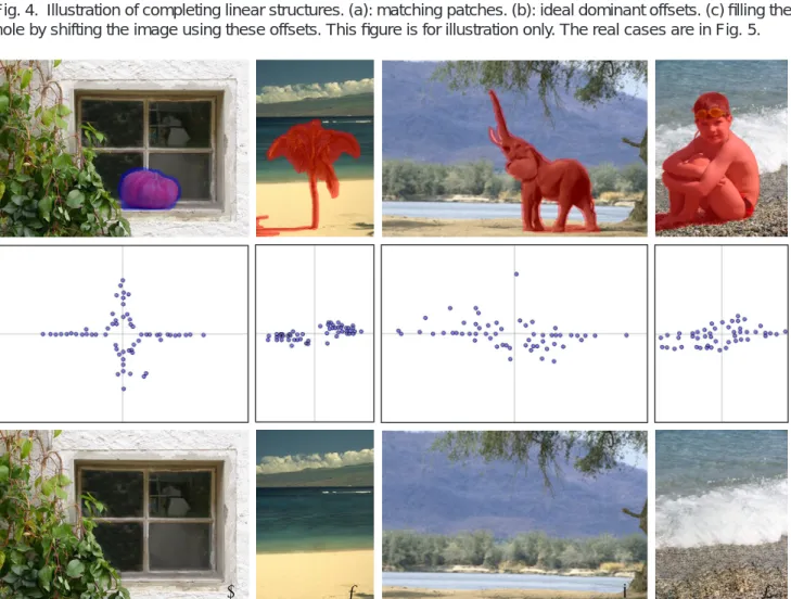
Ω offsets (a) u v (b) Ω shift (c)

Fig. 4. Illustration of completing linear structures. (a): matching patches. (b): ideal dominant offsets. (c) filling the hole by shifting the image using these offsets. This figure is for illustration only. The real cases are in Fig. 5.

(a) (b) (c) (d)

u

v

v

u

v

u

v

u

Fig. 5. Linear structures. Top: input. Middle: dominant offsets. Bottom: the results obtained by our graph-based solution. (a) Long/thin objects. (b) Linear color edges. (c)(d) Linear textural edges.

hole under at least three situations: (i) linear struc-tures, (ii) regular/random texstruc-tures, and (iii) repeated objects.

3.2.1 Linear structures

As illustrated in Fig. 4(a), a patch on a linear structure can find its match that is also on this structure. The offsets statistics will exhibit a series of peaks along the direction of the structure (Fig. 4(b)). Here we use a dot to denote a dominant offset in the histogram. These offsets will shift the image along the linear structure, so can reliably complete the mission region.

Fig. 5 shows some real examples of this case. We find our method works well for the linear structures including long and thin objects (Fig. 5(a)), color edges

(Fig. 5(b)), and textural edges (Fig. 5(c)(d)). Note that our method is tolerant to the structures that are not salient (e.g., Fig. 5(c)) or that are not strictly straight (e.g., Fig. 5(d)); it is sufficient if the structures have a “trend” along one or a few directions.

3.2.2 Textures

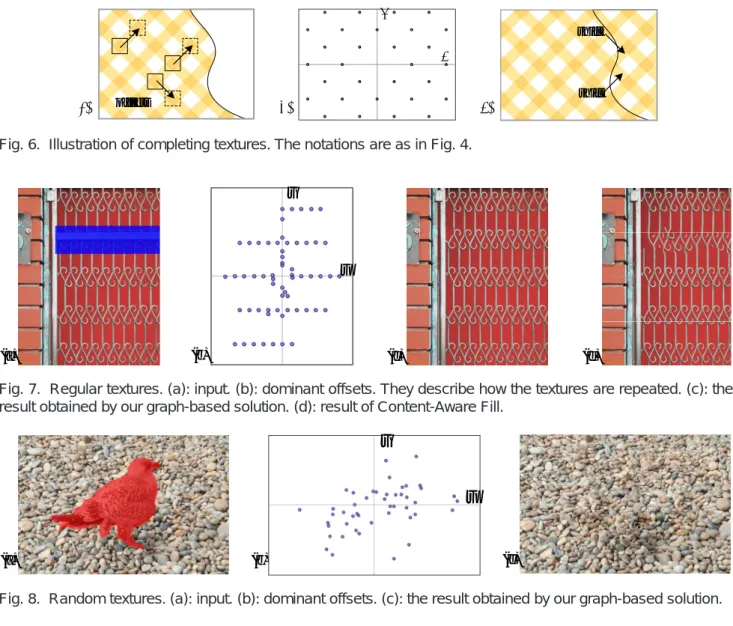
Textures can yield prominent patterns in the offset statistics. Ideally, a regular texture should generate a regular pattern of dominant offsets describing how the textures are repeated (Fig. 6). We can complete the texture by shifting the image using these offsets. Fig. 7 shows a real example of regular textures. Because the “period” of the regular textures can be larger than some predefined patch sizes, completing such textures

u v Ω offsets Ω shift shift (a) (b) (c)

Fig. 6. Illustration of completing textures. The notations are as in Fig. 4.

(a) (b) (c) (d)

u v

Fig. 7. Regular textures. (a): input. (b): dominant offsets. They describe how the textures are repeated. (c): the result obtained by our graph-based solution. (d): result of Content-Aware Fill.

(a) (b) (c)

u

v

Fig. 8. Random textures. (a): input. (b): dominant offsets. (c): the result obtained by our graph-based solution.

is a challenging task for other techniques like Content-Aware Fill [19] (Fig. 7(d)). For irregular textures, we find the dominant offsets generate random patterns (Fig. 8). In this case our method behaves just like the Graphcut texture algorithm [28].

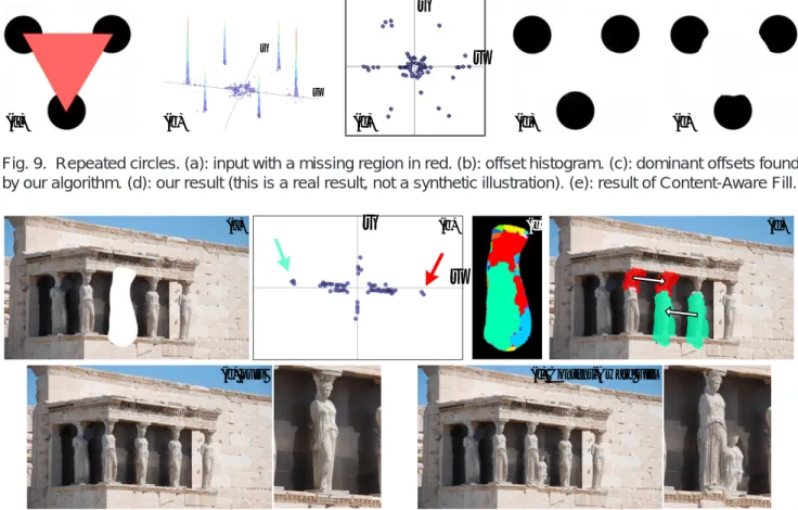
3.2.3 Repeated objects

Repeated objects can also generate prominent peaks in the offset statistics. This is helpful in synthesizing semantic content. As shown in Fig. 9, the partially missing circles yield peaks in the offsets that cor-respond to the relative positions of the circles. We can complete each circle by shifting another circle with these offsets. In Fig. 10 we show a real example in which our algorithm faithfully recovers a fully missing sculpture. We find that Content-Aware Fill might produce unsatisfactory results (see Fig. 9(e) and Fig. 10(f)), mainly because it is unaware of how the objects are repeated.

In sum, the offsets statistics can predict the struc-tures in the missing regions in the cases of linear

structures, textures, and repeated objects. Our method has the advantage that it need not consider the above cases separately. It can handle all of them or a mixture of them in the same framework.

3.3 Offsets Selection and the Graph-based Ener-gy Optimization

Our graph-based method has an energy function Eqn. (3) similar to the Shift-map method [17]. The main difference is that Shift-map allows all possible offsets. As a result, our solution space is a very small subset of the one of Shift-map. Theoretically, Shift-map can achieve a smaller energy than our method (this is observed in experiments). However, we find that the results of Shift-map may have unexpected bias, and their visual quality can be unsatisfactory even if their energy is much lower than ours.

In Fig. 11 we optimize the energy Eqn. (3) re-spectively using our selected K dominant offsets (Fig. 11(b)) and using all possible offsets (Fig. 11(c)). The later is the way of Shift-map [17] (except that [17] has an extra gradient smoothness term). As expected,

(a) (b) v u (c)

v

u

Fig. 9. Repeated circles. (a): input with a missing region in red. (b): offset histogram. (c): dominant offsets found by our algorithm. (d): our result (this is a real result, not a synthetic illustration). (e): result of Content-Aware Fill.

(c) (d)

(b)

(a)

v

u

(e) ours (f) Content-Aware Fill

Fig. 10. Repeated objects. (a): input with a sculpture missing. (b): dominant offsets. The arrows indicate the offsets of the relative positions of the sculptures. (c): the label map obtained by graph-cuts: each color represents an offset. (d): the hole is mainly filled by copying the other sculptures, using the offsets indicated in (b). (e) our result and zoom-in. (f) result of Content-Aware Fill and zoom-in.

our energy (4.6×106) is much larger than the energy of Shift-map (1.1 ×106). But our result is visually superior.

We investigate this unexpected phenomenon through the graph-cuts label maps (Fig. 11(b)(c)). We find that with a huge number of offsets, the Shift-map method can decrease the energy by “inserting” a great number of insignificant labels into the seam (see the zoom-in of Fig. 11(c)). These labels correspond to a few isolated pixels that occasionally “connect” the content on both sides of the seam. When the offset candidates are in a great number, these “occasional” pixels are not rare. We further observe that this problem is inherent and cannot be safely avoided by a hierarchical solver [17] (Fig. 11(d)) or by combining the gradient smoothness term (Fig. 11(e), obtained from the authors’ demo [32]).

On the contrary, our method is less influenced by this problem (Fig. 11(b)). Actually, an ideal exemplar-based method should fill the missing region by copy-ing large segments (like patches or regions). This means that only a few offsets should take effect, which is ensured by our method. The above experiments and analysis indicate that reliably limiting the solution space is important for improving the quality in image

completion.

Although the dominant offsets selected by our method can improve the quality (and also speed), it is non-trivial to select a few reliable candidate offsets (e.g., 60) out of all possible ones (usually 104−106). We compare some naive offset selection methods in Fig. 12. We generate the same number (K = 60) of offsets, either on a regular grid (Fig. 12(b)), randomly (Fig. 12(c)), or by our method (Fig. 12(d)). We observe that the alternative methods cannot produce satisfac-tory results, because the predefined offsets do not capture sufficient information to predict the missing structures.

3.4 Patch Sizes for the Offsets Statistics

Most exemplar-based methods (except [17]) involve the issue of setting suitable patch sizes. Our graph-based energy does not rely on patch representations as in [17]; the patch sizes only impact the computation of the offsets statistics (Eqn. 1). As analyzed above, the dominant offsets in the statistics are mainly deter-mined by how the patterns are repeated in the known regions. Such repeatedness is insensitive to the patch sizes.

(c) E = 1.1 (d) E = 1.9 (e)

(a) (b) E = 4.6

Fig. 11. Offsets sparsity and optimized energy. (a): input. (b): our graph-based result and the label map. Energy: E= 4.6(×106), running time:t= 0.5s. (c): the result using all possible offsets.E= 1.1(×106),t= 4300s. (In this case the number of labels isK = 3.8×105, and the number of unknown pixels isN = 2.2×104.) (d): the result of a hierarchical solver [17].E = 1.9(×106),t = 83s. (e): the result from the authors’ demo [32] (with gradient smoothness terms). (e) u v (d) (c) (b) (a)

Fig. 12. Comparisons of offsets selection methods. (a): input. (b): the result of regularly spaced offsets. (c): the result of randomly distributed offsets. (d): our result. (e): our offsets. The dash line indicates the offsets used to complete the structure of the roof.

In Fig. 13 we show two examples using our graph-based solution. Here we test w×w = 4×4, 8×8, 16×16,24×24, and32×32patches used for computing the offsets statistics. We can see that our method can produce visually plausible results in a very side spectrum of patch sizes. This experiment shows that our method is very robust to patch sizes. In all other experiments in this paper, we fix the patch size as 8×8.

4

I

D

In this section we elaborate the implementation de-tails.

4.1 Computing the Statistics

To efficiently matching the patches as in Eqn. (1), we apply a nearest-neighbor field algorithm in [26] with a slight modification: to handle the non-nearby constraint (|s| > τ), before computing the difference between a pair of patches we first check their spatial distance and reject them if the constraint is disobeyed. We perform this matching step in a rectangular region centered around the bounding box of the hole. This rectangle is 3 times larger (in length) than this bounding box. The purpose of using such a rectangu-lar region is to avoid unreliable statistics if the hole is too small in practical applications (in most examples in this paper this region is the entire image because the holes are large). The thresholdτ in Eqn. (1) is set

4x4 patches 8x8 patches

16x16 patches 32x32 patches

input _{4x4 patches 8x8 patches}

16x16 patches 32x32 patches

input

24x24 patches 24x24 patches

Fig. 13. Image completion results obtained by our graph-based solution, using various patch sizes for computing the statistics of patch offsets.

as ₁₅1 max(w,h) where w and h are the width and height of this region. We downsample this region to 800×600 pixels if it is larger than this size. Then we use 8×8 patches to perform the matching step2_{. This} step takes<0.1s.

Given the nearest-neighbor fields(x), we compute the 2-d histogram h(u, v) as in Eqn. (2). We smooth this histogram by a Gaussian filter (σ=√2). In this smoothed histogram, we consider a “peak” as a bin whose magnitude is locally maximal inside a 9×9 window. The highest K peaks are picked out, and their corresponding offsets give the offset candidates {si}Ki=1 that will be used in the image completion

algorithms.

4.2 The Graph-based Method

We adopt a two-scale solver in our graph-based method (Sec 2.2.1). We first downsample the rectan-gular region (by a scale l) to 800×600 pixels if it is larger than this size. Then we build a graph as in Eqn. (3) and optimize it using graph-cuts [21]. We use the public code of the multi-label graph-cuts in [33]. Its time complexity is O(N K), where N is the number of unknown pixels and K is the number of labels. The time of this graph-cuts step is 0.2-0.5 seconds for an 800×600 image with 10-20% pixels missing. As a comparison, it takes over one hour to solve such an 800×600 image if all possible offsets are allowed at this scale (K=104-106, like Fig. 11(c)), or tens of seconds using a hierarchical solver [17] with the coarsest level as small as 100×100 pixels (like Fig. 11(d)). Thus our method is 1-2 orders of magnitude faster than Shift-map [17].

2. The method in [26] only supports patch sizes4k×4kfor some integerk. When computing the offset statistics, we need not use a (2r+ 1)×(2r+ 1)patch that centered at a certain pixel; instead, we can represent the spatial coordinates of a patch by its top-left corner. This representation is also adopted in the public codes of [18] and [25].

We upsample the above resulting label map to the full resolution by nearest-neighbor interpolation and multiply the offsets by l. To correct small misalign-ments, we optimize a cost similar to Eqn. (3) in the full resolution. We allow each pixel to take 5 offsets: the upsampled offset and 4 relative offsets: if the upsampled shift iss = (u, v), then the other 4 shifts are (u± ₂l, v) and (u, v± ₂l). In this cost function we only treat the pixels as unknowns if they are in l

2-pixel around the seams. This upsampling takes <0.1s for typical 2Mp images. We have also tested our graph-based method in full resolution without downsampling, and found the visual qualities are similar to the two-scale solver. We adopt the two-scale solver because it is faster.

Finally a Poisson fusion [29] is applied to hide the possibly visible seams. We adopt a recentO(N) time Poisson solver proposed in [34]. In our implementa-tion it takes 50ms per Megapixel.

4.3 The Matching-based Method

As in [14], [18], we adopt a multi-scale solver in our matching-based method (Sec 2.2.2). We build an image pyramid of L levels using a scaling factor 2, with a fixed coarsest size (≥ 100×100). We start the EM algorithm from the coarsest level, with an initialization discussed below. The result of a coarser level is interpolated into the next finer level. We interpolate the color image and at the next level start from the E-step. (Alternatively, we can interpolate the nearest neighbor field and at the next level start from the M-step. We find the former way is better at hiding the seams.) We run 20 iterations of EM steps in the coarsest level, 2 iterations in the finest level, and 5 iterations in other levels.

The result of the matching-based method is sensi-tive to the initialization. We have tested two ways of

Content-Aware Fill ours (matching-based)

ours (graph-based) input

Fig. 14. Comparisons with Content-Aware Fill. From left to right: input, our graph-based results, our matching-based results, and results of Content-Aware Fill. The artifacts are highlighted by the arrows. Image size (from top to down): 0.12Mp, 0.2Mp, 0.26Mp, 0.6Mp, 2Mp, 4Mp, 10Mp. The running time is in Fig. 15.

initializing at the coarsest level: using the Poisson e-quation [29] to roughly propagate colors and generate a smoothed guess, or use our graph-based solution to generate a structural guess. We find the second way is more robust and we report the results using this way.

Unlike the graph-based method, the matching-based method requires to set a patch size in its cost function (7). We fixed this size as w ×w = 9×9 throughout this paper, although in some cases we find

adjusting this size can give better results.

5

EXPERIMENTAL

RESULTS

All experiments are run on a PC with an Intel Core i7 3.0GHz CPU and 8G RAM. We recommend view-ing the supplementary video to experience the user interactions and speed.

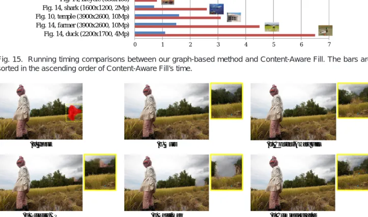
0 1 2 3 4 5 6 7 Fig. 7, door (300x400) Fig. 14, lady (300x400) Fig. 14, lion (500x400) Fig. 14, cat (1000x600) Fig. 1, sculpture (800x600) Fig. 14, bicycle (650x400) Fig. 14, shark (1600x1200, 2Mp) Fig. 10, temple (3900x2600, 10Mp) Fig. 14, farmer (3900x2600, 10Mp) Fig. 14, duck (2200x1700, 4Mp) Ours (graph-based) Content-Aware Fill

Running time / seconds

Fig. 15. Running timing comparisons between our graph-based method and Content-Aware Fill. The bars are sorted in the ascending order of Content-Aware Fill’s time.

(a) Input

(f) Criminisi et al.’s (e) Shift-map

(b) Ours (c) Content-Aware Fill

(d) Priority-BP

Fig. 16. Comparisons with state-of-the-art methods. (a) Input (640×430). (b) Ours (graph-based, 0.18s). (c) Content-Aware Fill (0.3s). (d) Priority-BP [15] (117s). (e) Shift-map [17] (13s). (f) Criminisi et al.’s [7] (6.9s).

5.1 Comparison with Content-Aware Fill

The tool Content-Aware Fill in Adobe Photoshop is reported [19] as an implantation partially based on [11], [18]. We believe it is a well-tuned, optimized, and perhaps enhanced implementation. It has shown compelling quality and speed in many practices. In this subsection we compare with this tool3_.

Some comparisons have been shown in the pre-vious sections (Fig. 1, 7, 9, and 10). In Fig. 14 we show more examples using our both methods (graph-based and matching-(graph-based). In all these examples our methods complete the images using as few asK= 60 pre-selected offsets. Our both methods generate high-quality results, whereas the Content-Aware Fill pro-duces noticeable artifacts in these examples.

Fig. 15 shows the running time of our graph-based solution and the Content-Aware Fill. Both methods are using quad cores. (Our graph-based method ben-efits less than Content-Aware Fill in multi-core, mainly because in Content-Aware Fill the EM algorithm and

3. We have also tested an implementation of [11], [18] given by the public code in [35], but we find it is non-trivial to tune universally acceptable parameters.

PatchMatch are fully parallelized, but the graph-cuts algorithm we used is not. In our graph-based method, the parallelism is only for matching patches and Pois-son blending.) For small images where the two-scale solution does not take effect (the first six examples in Fig. 15), our graph-based method is slightly faster than Content-Aware Fill. But for mega-pixel images our graph-based method is 2-5 times faster. This is because matching patches in mega-pixel images can be slow at finer scales. Our matching-based method takes about 50-100% more time than our graph-based method.

5.2 Comparisons with Other State-of-the-art Methods

In Fig. 16 we further compare with Priority-BP [15], Shift-map [17], and Criminisi et al.’s method [7]. Our method faithfully recovers the texture edges here, and is much faster than the other three methods (see the caption in Fig. 16). More comparisons are in the supplementary materials4_.

input ours Content-Aware Fill Priority-BP

Fig. 17. A comparison with Priority-BP [16]. For this 256×163 image Priority-BP takes 40s in a well parallelized quad-core implementation, while our graph-based method takes 0.09s.

input ours Shift-map

Fig. 18. A comparison with Shift-map [17]. In the zoom-in we show how Shift-map behaves near inconsistent seams.

ours (matching-based) ours (graph-based)

input input ours (graph-based) ours (matching-based)

Fig. 19. More results of images from previous papers [8], [13]. These images are around400×300. Our methods complete each image in less than 0.3 seconds.

Fig. 17 shows a comparison with Priority-BP [15]. This method optimizes an MRF using the BP algo-rithm with on-the-fly label pruning. Its running time for this 256×163-pixel image is 40s using a well par-allelized quad-core implementation, while our graph-based method takes 0.09s. Also note Priority-BP can-not recover the pattern in the lamp in this example.

Fig. 18 shows a comparison with Shift-map [17]. As also in Fig. 11, Shift-map cannot preserve the structure in this case. We can see (in zoom-in) how this method conceals a seam when the content is not consistent on both sides of this seam. This result is obtained from the authors’ on-line demo [32]. We tried various parameter settings but observed similar artifacts.

5.3 More Results and Limitations

In Fig. 19 we show more results in the example images from previous papers [8], [13]. In Fig. 20 we show an example of removing multiple small objects in a large image. In Fig. 21 we show two examples of completing panoramic images.

Limitations.Our methods may fail when the desired offsets do not form dominant statistics. Fig. 22(b) show a failure case. We can partially solve this prob-lem by manually introducing offsets. E.g., we can paint an extra stroke on the image (Fig. 22(d)), and treat this image as a new source for patch statistics. This stroke contributes to the statistics and overcomes the problem (Fig. 22(e)). Some other failure examples are in the supplementary materials.

6

CONCLUSION

In this paper we have presented novel statistics of patch offsets. We have demonstrated the effects of these statistics for image completion using both graph-based and matching-based methods.

Natural image statistics are essential for many computer vision problems. Gradient-domain statistics have been applied in denoising [36], deconvolution [37], and diffusion-based inpainting [3]. Patch-domain statistics have been shown very successful in denois-ing [36] and super-resolution [38]. We believe our statistics of patch offsets, as a kind of natural image

input objects to be removed our result zoom-in

Fig. 20. Removing multiple small objects from a large image (10Mp). The objects are removed sequentially. The results are obtained by our graph-based solution.

ours (matching-based) ours (graph-based)

input

Fig. 21. Our results for completing panoramic images. Our graph-based method takes 1.1s in the top image (3200×2000pixels) and 0.97s in the bottom image (2600×1800pixels).

(a) input (b) ours (c) Content-Aware Fill (d) modified input (e) ours on (d)

Fig. 22. Failure of the statistics. (a) Input. (b) Our graph-based result. (c) Result of Content-Aware Fill. (d) An extra stroke is casually painted on the image. (e) Our graph-based result of (d).

statistics, will find more applications in the future (e.g., [23], [24]).

The usage of the patch offsets implies that we only consider translations of patches for image completion. Recently, there are studies [39], [35], [40] on using more complex transforms like scaling, rotation, reflec-tion, and their combinations. It will be interesting to investigate the statistics in these higher dimensional transformation spaces. We leave this problem for fu-ture study.

R

[1] M. Bertalmio, G. Sapiro, V. Caselles, and C. Ballester, “Image inpainting,” in ACM Transactions on Graphics, Proceedings of ACM SIGGRAPH, 2000, pp. 417–424.

[2] C. Ballester, M. Bertalmio, V. Caselles, G. Sapiro, and J. Verder-a, “Filling-in by joint interpolation of vector fields and gray levels,” IEEE Transactions on Image Processing (TIP), pp. 1200– 1211, 2001.

[3] A. Levin, A. Zomet, and Y. Weiss, “Learning how to inpaint from global image statistics,” in Proceedings of the IEEE Interna-tional Conference on Computer Vision (ICCV), 2003, pp. 305–312. [4] M. Bertalmio, L. Vese, G. Sapiro, and S. Osher, “Simultaneous structure and texture image inpainting,” in Proceedings of the IEEE Conference on Computer Vision and Pattern Recognition (CVPR), 2003.

[5] S. Roth and M. J. Black, “Fields of experts: a framework for learning image priors,” in Proceedings of the IEEE Conference on Computer Vision and Pattern Recognition (CVPR), 2005, pp. 860–867.

[6] A. A. Efros and T. K. Leung, “Texture synthesis by non-parametric sampling,” in Proceedings of the IEEE International Conference on Computer Vision (ICCV), 1999, pp. 1033–1038. [7] A. Criminisi, P. Perez, and K. Toyama, “Object removal by

exemplar-based inpainting,” in Proceedings of the IEEE Confer-ence on Computer Vision and Pattern Recognition (CVPR), 2003.

[8] I. Drori, D. Cohen-Or, and H. Yeshurun, “Fragment-based im-age completion,” in ACM Transactions on Graphics, Proceedings of ACM SIGGRAPH, 2003, pp. 303–312.

[9] J. Jia and C.-K. Tang, “Image repairing: Robust image synthesis by adaptive nd tensor voting,” in Proceedings of the IEEE Conference on Computer Vision and Pattern Recognition (CVPR), vol. 1. IEEE, 2003, pp. I–643.

[10] ——, “Inference of segmented color and texture description by tensor voting,” IEEE Transactions on Pattern Analysis and Machine Intelligence (TPAMI), vol. 26, no. 6, pp. 771–786, 2004. [11] Y. Wexler, E. Shechtman, and M. Irani, “Space-time video completion,” in Proceedings of the IEEE Conference on Computer Vision and Pattern Recognition (CVPR), 2004.

[12] J. Sun, L. Yuan, J. Jia, and H.-Y. Shum, “Image completion with structure propagation,” in ACM Transactions on Graphics, Proceedings of ACM SIGGRAPH, 2005, pp. 861–868.

[13] Y. Wexler, E. Shechtman, and M. Irani, “Space-time completion of video,” IEEE Transactions on Pattern Analysis and Machine Intelligence (TPAMI), pp. 463–476, 2007.

[14] D. Simakov, Y. Caspi, E. Shechtman, and M. Irani, “Summariz-ing visual data us“Summariz-ing bidirectional similarity,” in Proceed“Summariz-ings of the IEEE Conference on Computer Vision and Pattern Recognition (CVPR), 2008.

[15] N. Komodakis and G. Tziritas, “Image completion using global optimization,” in Proceedings of the IEEE Conference on Computer Vision and Pattern Recognition (CVPR), 2006, pp. 442– 452.

[16] ——, “Image completion using efficient belief propagation via priority scheduling and dynamic pruning,” IEEE Transactions on Image Processing (TIP), pp. 2649–2661, 2007.

[17] Y. Pritch, E. Kav-Venaki, and S. Peleg, “Shift-map image editing,” in Proceedings of the IEEE International Conference on Computer Vision (ICCV), 2009, pp. 151–158.

[18] C. Barnes, E. Shechtman, A. Finkelstein, and D. B. Goldman, “PatchMatch: A randomized correspondence algorithm for structural image editing,” in ACM Transactions on Graphics, Proceedings of ACM SIGGRAPH, 2009, pp. 1–8.

[19] Adobe Systems Inc, “www.adobe.com/technology/graphics/ content aware fill.html,” 2009.

[20] K. P. Murphy, Y. Weiss, and M. I. Jordan, “Loopy belief propagation for approximate inference: An empirical study,” in Proceedings of the Conference on Uncertainty in Artificial Intel-ligence (UAI). Morgan Kaufmann Publishers Inc., 1999, pp. 467–475.

[21] Y. Boykov, O. Veksler, and R. Zabih, “Fast approximate energy minimization via graph cuts,” IEEE Transactions on Pattern Analysis and Machine Intelligence (TPAMI), pp. 1222–1239, 2001. [22] K. He and J. Sun, “Statistics of patch offsets for image com-pletion,” in Proceedings of the European Conference on Computer Vision (ECCV). Springer-Verlag, 2012, pp. 16–29.

[23] Z. Chen, H. Jin, Z. Lin, S. Cohen, and Y. Wu, “Large displace-ment optical flow from nearest neighbor fields,” in Proceedings of the IEEE Conference on Computer Vision and Pattern Recognition (CVPR), 2013.

[24] Y. Zhang, J. Xiao, J. Hays, and P. Tan, “Framebreak: Dramatic image extrapolation by guided shift-maps,” in Proceedings of the IEEE Conference on Computer Vision and Pattern Recognition (CVPR), 2013.

[25] S. Korman and S. Avidan, “Coherency sensitive hashing,” in Proceedings of the IEEE International Conference on Computer Vision (ICCV), 2011, pp. 1607–1614.

[26] K. He and J. Sun, “Computing nearest-neighbor fields via propagation-assisted kd-trees,” in Proceedings of the IEEE Con-ference on Computer Vision and Pattern Recognition (CVPR), 2012. [27] A. Agarwala, M. Dontcheva, M. Agrawala, S. Drucker, A. Col-burn, B. Curless, D. Salesin, and M. Cohen, “Interactive digital photomontage,” in ACM Transactions on Graphics, Proceedings of ACM SIGGRAPH, 2004, pp. 294–302.

[28] V. Kwatra, A. Sch ¨odl, I. Essa, G. Turk, and A. Bobick, “Graph-cut textures: image and video synthesis using graph “Graph-cuts,” in ACM Transactions on Graphics, Proceedings of ACM SIGGRAPH, 2003, pp. 277–286.

[29] P. P´erez, M. Gangnet, and A. Blake, “Poisson image edit-ing,” in ACM Transactions on Graphics, Proceedings of ACM SIGGRAPH, 2003, pp. 313–318.

[30] T. Liu, J. Sun, N.-N. Zheng, X. Tang, and H.-Y. Shum, “Learn-ing to detect a salient object,” in Proceed“Learn-ings of the IEEE

Conference on Computer Vision and Pattern Recognition (CVPR), 2007.

[31] M. Zontak and M. Irani, “Internal statistics of a single natural image,” in Proceedings of the IEEE Conference on Computer Vision and Pattern Recognition (CVPR), 2011, pp. 977–984.

[32] Shift-map On-line Demo, “www.vision.huji.ac.il/shiftmap/.” [33] Multi-label Graph Cuts, “http://vision.csd.uwo.ca/code/.” [34] Z. Farbman, R. Fattal, and D. Lischinski, “Convolution

pyra-mids,” in ACM Transactions on Graphics, Proceedings of ACM SIGGRAPH Asia, 2011.

[35] A. Mansfield, M. Prasad, C. Rother, T. Sharp, P. Kohli, and L. V. Gool, “Transforming image completion,” British Machine Vision Conference (BMVC), August 2011.

[36] V. Katkovnik, A. Foi, K. Egiazarian, and J. Astola, “From local kernel to nonlocal multiple-model image denoising,” International Journal of Computer Vision (IJCV), 2010.

[37] R. Fergus, B. Singh, A. Hertzmann, S. T. Roweis, and W. T. Freeman, “Removing camera shake from a single photo-graph,” in ACM Transactions on Graphics, Proceedings of ACM SIGGRAPH, 2006, pp. 787–794.

[38] D. Glasner, S. Bagon, and M. Irani, “Super-resolution from a single image,” in Proceedings of the IEEE International Conference on Computer Vision (ICCV), 2009.

[39] C. Barnes, E. Shechtman, D. B. Goldman, and A. Finkelstein, “The generalized patchmatch correspondence algorithm,” in Proceedings of the European Conference on Computer Vision (EC-CV). Springer, 2010, pp. 29–43.

[40] S. Darabi, E. Shechtman, C. Barnes, D. B. Goldman, and P. Sen, “Image Melding: Combining Inconsistent Images using Patch-based Synthesis,” in ACM Transactions on Graphics, Proceedings of ACM SIGGRAPH, 2012.

Kaiming He received the BS degree from the

Academic Talent Program, Physics Depart-ment, Tsinghua University in 2007, and the PhD degree from the Department of Infor-mation Engineering, the Chinese University of Hong Kong in 2011. He joined Microsoft Research Asia in 2011. His research inter-ests include computer vision and computer graphics. He has won the Best Paper Award at the IEEE Conference on Computer Vision and Pattern Recognition (CVPR) 2009.

Jian Sun got the BS degree, MS degree and

Ph.D degree from Xian Jiaotong University in 1997, 2000 and 2003. He joined Microsoft Research Asia in July, 2003. His current t-wo major research interests are interactive computer vision (user interface + vision) and internet computer vision (large image collec-tion + vision). He is also interested in stere-o matching and cstere-omputatistere-onal phstere-otstere-ography. He has won the Best Paper Award at the IEEE Conference on Computer Vision and Pattern Recognition (CVPR) 2009.