Development and Application of Hybrid Wray-Agarwal Turbulence Model and Large-Eddy Simulation

(1)

Washington University in St. Louis

Washington University Open Scholarship

Engineering and Applied Science Theses &

Dissertations McKelvey School of Engineering

Summer 8-15-2018

Development and Application of Hybrid

Wray-Agarwal Turbulence Model and Large-Eddy

Simulation

Xu Han

Washington University in St. Louis

Follow this and additional works at:https://openscholarship.wustl.edu/eng_etds

Part of theEngineering Commons, and thePhysics Commons

This Dissertation is brought to you for free and open access by the McKelvey School of Engineering at Washington University Open Scholarship. It has been accepted for inclusion in Engineering and Applied Science Theses & Dissertations by an authorized administrator of Washington University Open Scholarship. For more information, please [email protected].

Recommended Citation

Han, Xu, "Development and Application of Hybrid Wray-Agarwal Turbulence Model and Large-Eddy Simulation" (2018).Engineering and Applied Science Theses & Dissertations. 363.

(2)

WASHINGTON UNIVERSITY IN ST. LOUIS School of Engineering & Applied Sciences

Department of Mechanical Engineering & Material Science

Dissertation Examination Committee: Dr. Ramesh Agarwal, Chair

Dr. Kenneth Jerina Dr. Mark Meacham

Dr. David Peters Dr. Palghat Ramachandran

Development and Application of Hybrid Wray-Agarwal Turbulence Model and Large-Eddy Simulation

by Xu Han

A dissertation presented to The Graduate School of Washington University in

partial fulfillment of the requirements for the degree

of Doctor of Philosophy

August 2018 St. Louis, Missouri

(3)

(4)

ii

List of Figures

Figure 2.1: Flow past a circular cylinder at different Reynolds numbers. ... 7

Figure 4.1: Decaying Isotropic Turbulence test for WA-DES model. ... 20

Figure 4.2: Flow past a flat plate in zero pressure gradient [20]. ... 22

Figure 4.3: Comparison of computed skin friction distribution on the flat plate using the WA-DES model with the experimental data. ... 22

Figure 4.4: Comparison of computed pressure distribution with WA-DES model on the surface of NACA 0012 airfoil with experimental data. ... 23

Figure 4.5: Geometry of NASA wall-mounted hump, computational domain and boundary conditions. ... 24

Figure 4.6: Comparison of pressure distribution on the surface of the hump... 24

Figure 4.7: Comparison of Skin-Friction distribution on the surface of the hump... 25

Figure 4.8: Comparison of velocity profiles from WA-DES model and experimental values at various locations on the hump. ... 26

Figure 4.9: Comparison of velocity profiles from WA model and experimental values at various locations on the hump. ... 26

Figure 4.10: Comparison of velocity profiles from SA model and experimental values at various locations on the hump. ... 27

Figure 4.11: Geometry of backward facing step, computational domain and boundary conditions [20]. ... 28

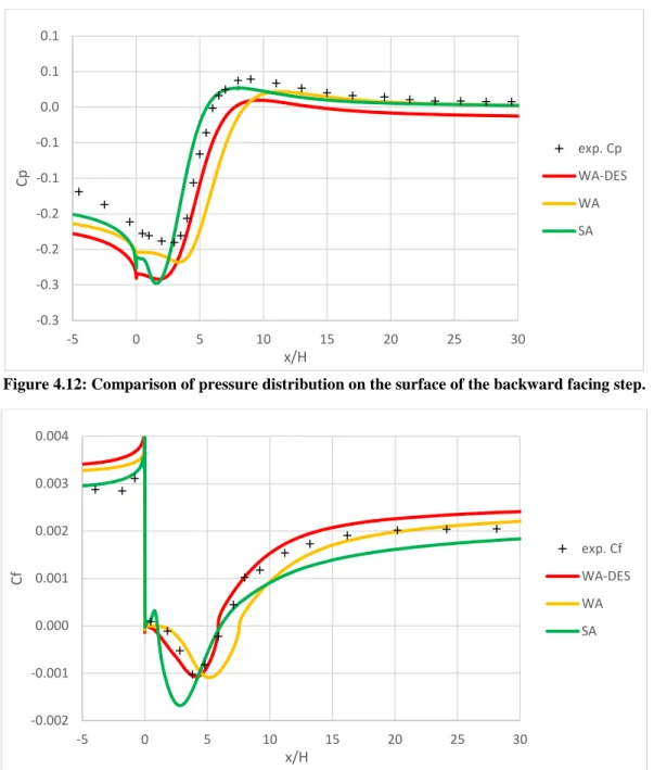
Figure 4.12: Comparison of pressure distribution on the surface of the backward facing step. ... 29

Figure 4.13: Comparison of Skin-Friction distribution on the surface of the backward facing step. ... 29

Figure 4.14: Comparison of velocity profiles from WA-DES model and experimental values at various locations on the step. ... 30

Figure 4.15: Comparison of velocity profiles from WA model and experimental values at various locations on the step. ... 30

Figure 4.16: Comparison of velocity profiles from SA model and experimental values at various locations on the step. ... 31

Figure 4.17: Geometry of the asymmetric plane diffuser [23]. ... 32

Figure 4.18: Comparison of pressure distribution on the top wall of the diffuser. ... 32

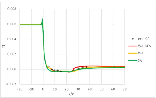
Figure 4.19: Comparison of pressure distribution on the bottom wall of the diffuser... 33

Figure 4.20: Comparison of Skin-Friction distribution on the top wall of the diffuser. ... 33

Figure 4.21: Comparison of Skin-Friction distribution on the bottom wall of the diffuser. ... 34

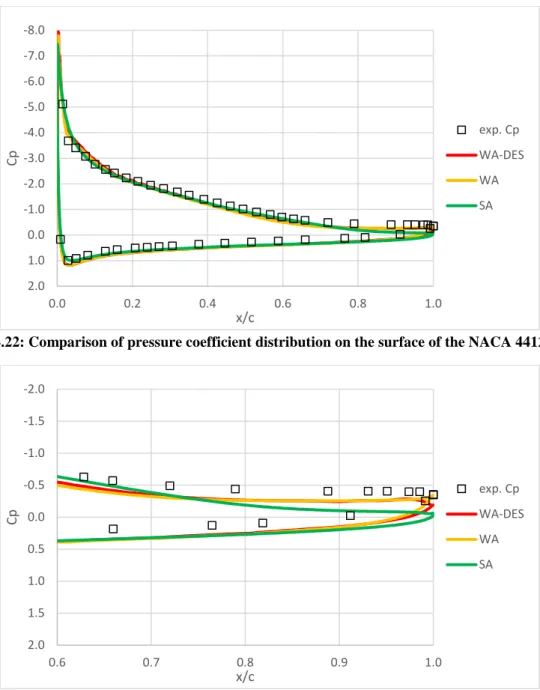
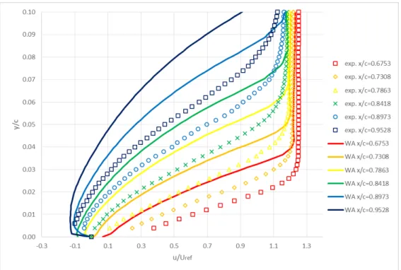
Figure 4.22: Comparison of pressure coefficient distribution on the surface of the NACA 4412 airfoil. ... 35

Figure 4.23: Zoomed-in-View of pressure coefficient distribution in the trailing edge separation region of NACA 4412 airfoil. ... 35

(8)

vi

Figure 4.24: Comparison of streamwise velocity profiles computed from WA-DES model and

experimental values at various locations on the NACA 4412 airfoil. ... 36

Figure 4.25: Comparison of streamwise velocity profiles computed from WA model and experimental values at various locations on the NACA 4412 airfoil. ... 37

Figure 4.26: Comparison of streamwise velocity profiles computed from SA model and experimental values at various locations on the NACA 4412 airfoil. ... 37

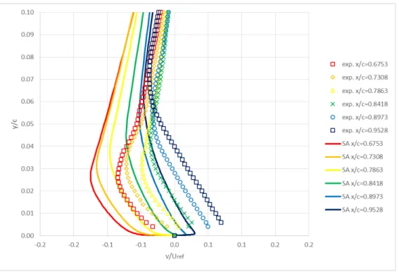
Figure 4.27: Comparison of vertical velocity profiles computed from WA-DES model and experimental values at various locations on the NACA 4412 airfoil. ... 38

Figure 4.28: Comparison of vertical velocity profiles computed from WA model and experimental values at various locations on the NACA 4412 airfoil. ... 38

Figure 4.29: Comparison of vertical velocity profiles computed from SA model and experimental values at various locations on the NACA 4412 airfoil. ... 39

Figure 4.30: Comparison of skin friction coefficient distribution on the period hill. ... 40

Figure 4.31: Comparison of pressure coefficient distribution on the period hill. ... 41

Figure 4.32: Comparison of pressure coefficient distribution on the top wall. ... 41

Figure 4.33: Comparison of velocity profiles on periodic hill... 42

Figure 4.34: Geometry and boundary conditions of transonic axisymmetric bump [20]. ... 43

Figure 4.35: Comparison of pressure coefficient distribution on the surface of the axisymmetric bump. ... 43

Figure 4.36: Comparison of vertical velocity profiles computed from WA-DES model and experimental values at various locations on the axisymmetric bump. ... 44

Figure 4.37: Comparison of vertical velocity profiles computed from WA model and experimental values at various locations on the axisymmetric bump. ... 45

Figure 4.38: Comparison of vertical velocity profiles computed from SA model and experimental values at various locations on the axisymmetric bump. ... 45

Figure 4.39: S-Duct geometry with planes of interest [29]. ... 46

Figure 4.40: Non-dimensional static pressure coefficient along the S- duct in NASA Glenn’s experiment [29]. ... 47

Figure 4.41: Comparison of experimental and computed pressure coefficients at 10º angular position. ... 48

Figure 4.44: Comparison of total pressure coefficient contours at AIP. ... 49

Figure 4.45: Comparison of Mach Number contours at AIP. ... 50

Figure 5.1: Grid Induced Separation by SA-DES model on an airfoil [31]. ... 52

Figure 5.2: Calibration of the SST-DDES constant on a flat plate with excessive refinement [34]. ... 54

(9)

vii

Figure 5.4: Comparison of RANS and LES length scales of different DES models inside the flat

plate boundary layer. ... 57

Figure 5.5: Comparison of pressure distribution on the surface of the hump... 58

Figure 5.6: Comparison of Skin-Friction distribution on the surface of the hump... 58

Figure 5.7: Comparison of velocity profiles from WA-IDDES model and experimental values at various locations on the hump. ... 59

Figure 5.8: Comparison of pressure distribution on the top wall of the diffuser. ... 60

Figure 5.9: Comparison of pressure distribution on the bottom wall of the diffuser... 61

Figure 5.10: Comparison of Skin-Friction distribution on the top wall of the diffuser. ... 61

Figure 5.11: Comparison of Skin-Friction distribution on the bottom wall of the diffuser. ... 62

Figure 5.12: Comparison of skin friction coefficient distribution on the period hill. ... 63

Figure 5.13: Comparison of pressure coefficient distribution on the period hill. ... 63

Figure 5.14: Comparison of pressure coefficient distribution on the top wall. ... 64

Figure 5.15: Comparison of velocity profiles on the periodic hill. ... 64

Figure 5.17:Comparison of pressure distribution on the surface of the backward facing step. .... 66

Figure 5.18:Comparison of velocity profiles computed from WA-IDDES model and experimental values at various locations on the backward facing step. ... 66

Figure 5.19: Comparison of pressure distribution on the surface of the curved backward facing step. ... 68

Figure 5.20:Comparison of skin-friction distribution on the surface of the curved backward facing step. ... 68

Figure 5.21: Comparison of vertical velocity profiles computed from hybrid models and LES values at various locations on the backward facing step. ... 69

Figure 5.22: Comparison of vertical velocity profiles computed from RANS models and LES values at various locations on the backward facing step. ... 69

Figure 5.23: Comparison of pressure coefficient distribution on the surface of the axisymmetric bump. ... 70

Figure 5.24: Comparison of vertical velocity profiles computed from WA-IDDES model and experimental values at various locations on the axisymmetric bump. ... 71

Figure 6.1: Comparison of velocity profile in the channel at Reτ = 182. ... 79

Figure 6.6: Comparison of velocity profile in turbulent channel at Reh = 80x106 at x=500. ... 82

Figure 6.7: Comparison of turbulent viscosity ratio in channel at Reh = 80x106 at x=500. ... 82

Figure 6.9: Comparison of Skin-Friction distribution on the surface of the backward facing step. ... 84

(10)

viii

Figure 6.10: Comparison of velocity profiles from WA2018-EB model and experimental data at various locations on the step. ... 84 Figure 6.11: Comparison of Skin-Friction distribution on the bottom surface of the periodic hill. ... 85 Figure 6.12: Comparison of pressure coefficient distribution on the bottom surface of the

periodic hill. ... 86 Figure 6.13: Comparison of pressure coefficient distribution on the top surface of the periodic hill. ... 86 Figure 6.14: Comparison of computed velocity profiles and experimental data at various

locations on the hill. ... 87 Figure 6.15: Comparison of pressure coefficient distribution on the surface of the axisymmetric bump. ... 88 Figure 6.16: Comparison of vertical velocity profiles computed from WA2018-EB model and experimental data at various locations on the axisymmetric bump. ... 89 Figure 7.1: Temperature profile in fluctuation measurement experiment [51]. ... 94

(11)

ix

List of Tables

Table 4.1: Comparison of flow separation and reattachment points of the axisymmetric bump. 43 Table 4.2: Comparison of flow separation and reattachment points for the S-Duct. ... 49 Table 5.1: Comparison of flow separation and reattachment points of the axisymmetric bump. 70 Table 6.1: Comparison of flow separation and reattachment points of the axisymmetric bump. 88 Table 7.1: Experimental data of fluctuation measurement experiment [51]. ... 94

(12)

x

Nomenclature

A = flow variable for demonstrating the hybrid scheme of WA-DES model

CFD = Computational Fluid Dynamics

Cf = skin friction coefficient Cp = pressure coefficient

c = hump length, NACA 4412 chord length, bump length DES = Detached-Eddy Simulation

DDES = Delayed Detached-Eddy Simulation D1 = NASA Glenn S-Duct inlet diameter d = distance to the nearest wall

𝑑𝑑̃ = DES length scale of SA-DES model

FDES = characteristic length scale ratio of DES model FIDDES = characteristic length scale ratio of IDDES model fd = shielding function of DDES model

fcomp,k = density fluctuation effects of SST k-ω model fcomp,R = density fluctuation effects of WA-DV model fR-S = relation function between R and S

f1 = blending function of Wray-Agarwal model fµ = wall damping function of Wray-Agarwal model

H = backward facing step height, diffuser inlet height h = periodic hill height

IDDES = Improved Delayed Detached-Eddy Simulation

(13)

xi

LES = Large Eddy Simulation

LR = turbulent length scale of WA2018-EB model lDES = characteristic length scale of DES model lDDES = characteristic length scale of DDES model lHYB = hybrid length scale of IDDES model

lk-ω = characteristic length scale of SST k-ω model

lLES = characteristic length scale of LES model lRANS = characteristic length scale of RANS model lref = reference length scale of WA2018-EB model M = Mach number

PR = transport variable of elliptic blending equation Pw = wall pressure

Qw = wall heat flux Tw = wall temperature

𝑇𝑇′ ₌ _{temperature fluctuation} R = undamped eddy viscosity, k/ω

RANS = Reynolds-Averaged Naiver-Stokes

Re = Reynolds number

S = mean strain rate magnitude

SA = Spalart-Allmaras

SST = Shear Stress Transport

s = NASA Glenn S-Duct centerline curve length

u = x-component of velocity

(14)

xii

W = mean vorticity magnitude

WA = Wray-Agarwal

y+ = non-dimensional wall distance

∆ = grid spacing

∆DES = grid spacing of DES model

∆IDDES = grid spacing of IDDES model

∆WN = grid spacing in wall normal direction ε = turbulent dissipation

ν = molecular kinematic viscosity

νT = turbulent viscosity

𝜈𝜈� = transport variable of Spalart-Allmaras model

ρ = density 𝜌𝜌̅ = mean density 𝜌𝜌′ ₌ _{density fluctuation}

𝜌𝜌′2 ₌ _{transport variable of density fluctuation equation} ω = specific turbulent dissipation rate

(15)

xiii

Acknowledgments

I sincerely appreciate the guidance from Dr. Agarwal during my research. This work could not be successfully conducted without unfailing trust, continuous encouragement and professional guidance from an excellent mentor.

I was delighted to receive the efforts and time of my committee members to read the dissertation and provide valuable comments.

I would like to thank my family for their constant love and support. And special thanks to all my friends in CFD lab that make our workplace wonderful.

I would also like to thank the staff of the MEMS department during my time at Washington University.

The financial support for this work was provided by a NASA EPSCoR Grant. It is gratefully acknowledged.

Computations were mainly performed using the facilities of the Washington University Center for High Performance Computing.

Xu Han

Washington University in St. Louis August 2018

(16)

(17)

xv

(18)

xvi

Abstract of the Dissertation

Development and Application of Hybrid Wray-Agarwal Turbulence Model and Large-Eddy Simulation

by Xu Han

Doctor of Philosophy in Mechanical Engineering Washington University in St. Louis, 2018

Research Advisor: Ramesh Agarwal

Rapid development in computing power in past five decades along with the development and progress in building blocks of Computational Fluid Dynamics (CFD) technology has made CFD an indispensable tool for modern engineering analysis and design of fluid-based products and systems. For CFD analysis, Reynolds-Averaged Navier-Stokes (RANS) equations are currently the most widely used fluid equations in the industry. RANS methods require modeling of turbulence effect (i.e. turbulence modeling) based on empirical relations and therefore often produce low accuracy results for many flows. In recent years, the Large Eddy Simulation (LES) approach has been developed which has shown promise of achieving higher accuracy, however it is computationally very intensive and therefore has remained limited to computing relatively simple flows from low to moderate Reynolds numbers. As a result, a hybrid technique called Detached Eddy Simulation (DES) has been proposed in recent years. This technique has shown improved accuracy and computational efficiency for solution of wide variety of complex turbulent flows. The goal of this dissertation has been to develop a DES model based on a

recently proposed very promising RANS model, known as the ‘Wray-Agarwal (WA)’ model and the LES. Decaying Isotropic Turbulence (DIT) case is computed to determine the coefficient in

(19)

xvii

the DES model by matching its energy spectrum with the Kolmogorov spectrum. The new WA-DES model (WA-DES model based on WA model) is applied to compute a wide variety of wall bounded separated flows to assess it accuracy and computational efficiency compared to the widely used RANS turbulence models in the industry, namely the Spalart-Allmaras (SA) and SST k-ω models. Improved Delayed-Detached Eddy Simulation (IDDES) and Elliptic Blending are also considered as further refinements of WA model to improve its accuracy.

(20)

1

Chapter 1: Introduction

1.1 Background and Motivation

Computational Fluid Dynamics (CFD) is playing an important role in modern engineering analysis and design including automobiles, aircrafts, turbomachinery, and many other industrial applications. Almost all flows in industrial applications are turbulent. After more than a century of concerted effort, accurate prediction of turbulent flows still remains a challenging problem even for incompressible wall bounded flows with separation. To date, the solution of Reynolds-Averaged Navier-Stokes (RANS) equations for simulating turbulent flows remains the most widely used approach in industry. The RANS equations include the so called ‘turbulent stresses’ that need to be modeled in order to achieve closure to the equations. Modeling of ‘turbulent stresses’ is called ‘turbulence modeling’ which introduces empiricism and is a major source of difficulty in accurately predicting the turbulent flows. In recent years, higher fidelity approaches namely the Large Eddy Simulation (LES) and Direct Numerical Simulation (DNS) have been developed which have shown promise, however they are computationally very intensive and therefore will remain limited to the computation of relatively simple flows at moderate to low Reynolds numbers respectively in the foreseeable future. As a result, in recent years, hybrid techniques which combine the best features of RANS and LES in a flow domain have been proposed; these techniques have shown improved accuracy and computational efficiency for the solution of 3D complex turbulent flows. These are called the “Detached Eddy Simulation (DES)” methods.

(21)

2

1.2 Objectives

The goal of this work is to develop a new DES model based on a recently developed very promising one equation turbulence model based on the k-ω closure, known as the ‘Wray -Agarwal (WA)’ model. The new DES model is designated as the ‘WA-DES’ model. In the boundary layer regions close to the wall, DES model solves the RANS equations while away from the wall in the complex separated flow regions, it employs LES where RANS equations are not quite accurate. In the literature, DES models have been developed based on the widely used one-equation Spalart-Allmaras (SA) model [1] and the two-equation SST k-ω model [2]. The development of WA-DES model requires the accurate determination of a modeling coefficient

CDES (which allows the switch between the RANS and LES in the flow) which is determined by

simulation of Decaying Isotropic Turbulence (DIT) and matching its energy spectrum with the Kolmogorov spectrum in both the inertial and viscous range. The WA-DES model is applied to compute a variety of wall bounded separated flows, namely the separated flows over a NASA hump and a backward facing step, and inside a diffuser and a S-Duct to assess it accuracy and computational efficiency compared to RANS turbulence models.

Another goal of this work is to refine the original WA model. Currently, the most widely used turbulence models in industry are the SA model and SST k-ω model. SA model provides robustness and efficiency for CFD simulations. SST k-ω model is used for relatively better accuracy compared to SA model. Both models were originally developed in 1980’s and continue to be updated until today. The newly developed WA model, which has been proven to be better in accuracy than SA model and competitive with SST k-ω model in accuracy for a wide variety of flows, still requires adjustments to some of the coefficients and other improvements and extensions due to its relatively very recent origin. In addition to its extension to WA-DES and

(22)

3

WA-IDDES, its baseline original formulation is improved by including a zero strain-rate

correction, a wall distance free approach formulation and an elliptic relaxation/blending method.

1.3 Outline

The goal of this dissertation is twofold: (1) To extend the WA model to create a validated hybrid WA/LES model, i.e. the WA-DES model and its other variations namely the WA-DDES and WA-IDDES models and (2) to improve the accuracy of original baseline WA model by including a zero strain-rate correction, a wall distance free formulation and an elliptic relaxation/blending method.

A brief summary of various chapters and their content is given below:

Chapter 2: Turbulence Modeling: This chapter briefly describe the concept of turbulent flows and turbulence modeling. The two main approaches for computing turbulent flows namely the Reynolds-Averaged Navier-Stokes (RANS) equations with turbulence models and the Large-Eddy Simulation (LES) with a sub-grid scale model are briefly described.

Chapter 3: Computational Fluid Dynamics: In this chapter, a brief introduction to

computational fluid dynamics (CFD) is given. In particular, the two main software employed in this dissertation for developing and testing the new models, namely the OpenFOAM and Dakota are briefly described. OpenFOAM is used to develop the new models and run the validation cases. Dakota is used to optimize the model coefficients. A brief description of hardware used for CFD calculations is also given.

(23)

4

Chapter 4: The WA-DES Model: This chapter gives a brief introduction of Detached-Eddy Simulation (DES), and the Wray-Agarwal (WA) turbulence model, which is combined with LES to derive the Wray-Agarwal Detached-Eddy Simulation (WA-DES) model. The model constant

CDES in WA-DES model is calibrated by performing the benchmark test case of Decaying

Isotropic Turbulence (DIT) and comparing the WA-DES energy spectrum with Kolmogorov energy spectrum both in inertial and viscous region. Several benchmark validation cases from NASA TMR are computed to show the benefits of this hybrid WA-DES model.

Chapter 5: The WA-IDDES Model: A brief introduction of two refinements to DES model, namely the Delayed Eddy Simulation (DDES) and the Improved Delayed Detached-Eddy Simulation (IDDES) is given in this chapter. DDES approach is discussed and is shown to be not very beneficial as extension of DES. IDDES approach is developed based on WA-DES model to derive the WA-IDWA-DES model. The capability of WA-IDWA-DES model is tested by computing a number of benchmark validation cases from NASA TMR.

Chapter 6: The Wall Distance Free and Elliptic Blending: This chapter describes several extensions to the original Wray-Agarwal model (WA2017) to improve its implementation and accuracy. The extensions include (1) modification to the model to remain accurate and robust under the special condition of zero strain-rate in the flow field, (2) a wall distance free (WDF) formulation to provide improved accuracy near curved surfaces, and (3) elliptic blending to improve the accuracy of wall bounded mildly separated flows. The WA model with all the three extensions (WA2018-EB model) is tested on several benchmark test cases.

Chapter 7: Summary and Future Work: This chapter provides a summary of the work accomplished in this dissertation, including modeling and testing of the WA-DES, WA-IDDES

(24)

5

and WA2018-EB models. The future work describes the density variance correction to the Wray-Agarwal model to extend its capability for computing high speed compressible flows.

(25)

6

Chapter 2: Turbulence Modeling

2.1 Turbulent Flow

2.1.1 Laminar and Turbulent Flow

The flow is laminar only at very low Reynolds numbers (the ratio of inertial force and viscous force). Such flows are encountered in very few engineering applications such as those involving very small sizes and velocities, e.g. droplets and bubbles, and in microfluidics and biological applications. In laminar flows, the flow is considered to move in laminas, and there is little transfer of momentum and energy between the adjacent layers of laminas. However, as the Reynolds number increases, chaotic or random fluctuations occur that result in low momentum diffusion, high momentum convection, and rapid variation in pressure and velocity in space and time in a fluid region. The laminar flows undergo transition to turbulent flows with an extremely complex flow behavior as the Reynolds number increases above a critical value. Both laminar and turbulent flows can be described by the laws of conservation of mass, momentum and energy which are expressed by the continuity equation, momentum equation and energy equation. The governing mass and momentum conservation equations for an incompressible fluid are shown in Eq. (1) below. 𝜕𝜕𝑢𝑢𝑗𝑗 𝜕𝜕𝜕𝜕𝑗𝑗 = 0 𝜌𝜌𝜕𝜕𝑢𝑢_{𝜕𝜕𝜕𝜕}𝑖𝑖+𝜌𝜌𝑢𝑢𝑗𝑗𝜕𝜕𝑢𝑢_{𝜕𝜕𝜕𝜕}𝑖𝑖 𝑗𝑗 = − 𝜕𝜕𝜕𝜕 𝜕𝜕𝜕𝜕𝑖𝑖 + 𝜕𝜕 𝜕𝜕𝜕𝜕𝑗𝑗�2𝜇𝜇𝑆𝑆𝑖𝑖𝑗𝑗� (1)

2.1.2 Separated Flow

Many wall bounded flows encounter separation of turbulent boundary layer attached to the surface because of adverse pressure gradient. When the flow separates, the boundary layer is detached from the solid surface and creates eddies and vortices in the separated flow region.

(26)

7

Depending upon the pressure gradient, the separation region can be small or massive. Pressure drag of the object often increases due to low pressure in the separation region. Separation is very common in industrial applications. For example, separation occurs on airfoils/wings at high angles of attack and behind automobiles and causes large increase in pressure drag. Additionally, at high Mach numbers, the separation can occur due to shock/boundary layer interaction in transonic, supersonic and hypersonic flow. Accurate prediction of wall bounded separated flows remains a challenging task for turbulence models.

Figure 2.1: Flow past a circular cylinder at different Reynolds numbers.

Figure 2.1 shows the evolution of separated flows behind a circular cylinder as Reynolds number increases. Computation of this flow at high Reynolds numbers remains a challenging task to date for all turbulence models used with RANS equations. It is also not possible to calculate the flow

(27)

8

at high Reynolds numbers using LES or DNS because of the inadequacy of the computational resources currently available. One of the main objectives of this thesis is to improve the accuracy of turbulence models for predicting wall bounded separated turbulent flows.

2.2 Turbulence Modeling

2.2.1 Background

Behavior of laminar flow is determined by a single length scale, which mainly comes from the boundaries of the flow region. If one can accurately describe the boundaries of a laminar flow region, the flow behavior in it can be calculated precisely using the Navier-Stokes equations. For very simple geometries and fully developed laminar flows, it has been possible to obtain a few exact analytical solutions of the Navier-Stokes. However, when the flow becomes turbulent, the turbulent fluctuations can only be fully characterized by an infinite number on length and time scales varying from very small to large values.

2.2.2 Reynolds-Averaged Navier-Stokes (RANS) Equations

Dating back to early 1900 since Osborne Reynolds, there have been three major approaches that have been developed to model and approximate mathematically the turbulent fluid behavior. The oldest developed in early 1900 is based on time-averaging of the Navier-Stokes equations which results in the Reynolds-Averaged Navier-Stokes (RANS) equations. RANS averaging results in the so called “turbulent stresses” or “Reynolds Stresses” which are unknown and require

modeling using empiricism. Thus, RANS equations are not closed; it is known as the “Closure Problem” in RANS equations. Closure of RANS equations requires empirical models for “Reynolds Stresses”; these models are called the “RANS Turbulence Models.” The solution of RANS equations with turbulence models to date remains the most widely used method in industry for solving the turbulent flows.

(28)

9

2.2.3 Large-Eddy Simulation (LES)

There are two other approaches that have been developed since 1980s which are more accurate than RANS equations in conjunction with a turbulence model but are computationally very intensive and are still not practical for industrial applications. These are known as the Large Eddy Simulation (LES) and the Direct Numerical Simulation (DNS). The Sub-Grid Scale (SGS) model is used in LES to reduce the computational cost. In LES, the velocity field is filtered to separate the motion of large and small eddies. Only the large eddies are resolved directly without modeling, however the smaller eddies require modeling. The models used to characterize the small eddies are called the Sub-Grid Scale (SGS) models. Most well-known among them are the Smagorinsky model [3] and Germano model [4] among others. LES has a much higher level of accuracy compared to RANS but is computationally expensive, especially for computing turbulent boundary layers. In DNS, all the length scales, from the largest down to the

Kolmogorov scale where the turbulent kinetic energy is dissipated to heat, the turbulent flow is resolved by solving the Navier-Stokes equations directly without any modeling. DNS is the most accurate method but has the highest computational cost and requires enormous computing power which is currently possible and affordable only for calculating flows at low Reynolds number for very simplest geometries [5]. As mentioned before, most of the industrial flows in complex 3D geometries are currently computed using the RANS equations with a turbulence model.

(29)

10

Chapter 3: Computational Fluid Dynamics

3.1 Introduction

Experimental and theoretical methods are the two main traditional approaches for solving the fluid mechanic and heat transfer problems. With the rapid development of digital computers since 1950’s. It is now feasible to solve almost routinely in most cases the ordinary and partial differential equations numerically. The numerical solution at the same time, has been aided by the software developments including Computer-Aided Design (CAD), finite-difference/finite-volume/finite-element methods and data reduction visualization techniques, etc. Making use of these developments in hardware and software, CFD has now become the third and the most widely used main method for solving fluid dynamics problems.

Currently, CFD has been successfully used in a large number of industrial applications and it now keeps on growing at a faster pace. The fundamental transport equations solved in a CFD code are being reinvestigated by data science methodology due to the availability of large data sets along with the development of statistical methods [6]. In addition, heterogenous systems implemented with accelerators like Graphical Processing Units (GPUs) have helped in

improving the runtime of the time-consuming parts (mostly the iterative matrix multiplications) using massive parallelization [7]. With the development of physical modeling,

mathematics/numerical methods and computer science, the future of CFD appear to be more promising than ever before.

3.2 Software

3.2.1 OpenFOAM

In this research, the CFD flow solver OpenFOAM (Open source Field Operation And

(30)

11

operating system. It was initially released in 2004 and continues to be developed by addition of all kind of CFD capability in complex fluid physics modeling, type of grids and numerical algorithms, and turbulence models. It includes the most well-known turbulence models namely the SA model, SST k-ω model, and k-ϵ model among others. It can therefore be used for wide range of applications, including incompressible and compressible turbulent flows, buoyancy-driven flows, multiphase flows, and application with heat transfer, combustion and particle dynamics etc.

In contrast to commercial CFD software such as ANSYS Fluent, COMSOL, STAR-CD etc., OpenFOAM provides the source code which makes it easy to modify it by adding needed capability to solve a particular problem. It has been developed in C++ programming language which has many good features like modularity and extensibility. Users can easily and effectively develop and test the new CFD capability. The commercial CFD software only provides the executable code which requires the development and implementation of a User Defined Function (UDF) to add new capability which is a tedious process.

In this work, all the simulations are performed using OpenFOAM, and the new models are developed and implemented as OpenFOAM libraries. Some of the simulation cases (e.g. flat plate, NASA hump, etc.) are also performed in ANSYS fluent, and FUN3D (NASA CFD code) to be verification of simulation result. All the three codes yield the same CFD results for flow quantities such as the velocity profiles, pressure coefficients and skin-friction coefficients in different flow configurations.

3.2.2 Dakota

In order to investigate and optimize the coefficients of new models developed in this work, another open source software called Dakota is used for optimization of the coefficients. Dakota

(31)

12

served as an interface between the CFD code and the iterative system analysis method. As a result, its flexibility and extensibility allow the user to analyze any “black box” even though the robustness is usually not guaranteed. The algorithms contained in Dakota include: gradient-based and non-gradient-based methods; uncertainty quantification with sampling, reliability, and stochastic expansion methods; parameter estimation with nonlinear least squares methods; and sensitivity/variance analysis with design of experiments and parameter study methods [8].

The effect of coefficients in WA model has been previously investigated using uncertainty qualifications based on non-intrusive Polynomial Chaos Expansion (PCE) method [9]. In this research, the coefficients of the new models are optimized by the NL2SOL algorithm in order to minimize the difference between the experimental data and the model outputs. The NL2SOL algorithm is a non-linear least-squares algorithm, which is significantly more efficient than generally used optimization algorithms when user can provide the gradients of each term in the sum-of-squares [8]. However, this algorithm can only provide the local optimization result. The global optimal result is approximated by dramatically changing the initial guess of the coefficient, but not applying any expensive general global optimizer such as a genetic algorithm.

3.3 Hardware

Most of the computations in this research have been performed on the computing cluster at the Center for High-Performance Computing (CHPC) of Mallinckrodt Institute of Radiology at Washington University School of Medicine in St. Louis [10]. CHPC provides access to high performance computing resources for computationally intensive scientific projects. The cluster contains 2,500 high speed CPU cores, 17TB of combined memory, 74 Tesla-class GPUs and 150TB of internal high speed shared storage. Software package (e.g. OpenFOAM) installation and code parallelization support is also provided via CHPC staff.

(32)

13

Chapter 4: The WA-DES Model

4.1 Introduction

4.1.1 Detached-Eddy Simulation

Detached-Eddy Simulation (DES) is a hybrid turbulence modeling method first proposed in 1997 by Spalart et al. [1], aimed at predicting the massive flow separation at high Reynolds number without a significant increase in computational cost. DES is a combination of RANS and LES methods. In the separation region, DES is designed to run in the LES mode; its turbulent

viscosity becomes a function of local grid spacing which is determined by a SGS model such as the Smagorinsky-Lilly model. Outside the separation regions, especially in the turbulent

boundary layer, DES runs in the RANS mode. As a result, DES only needs fine LES type grid in the separation region, and thus the high computational cost of LES computation in the boundary layer is avoided by running RANS equations on coarse grids.

The first DES model called DES97 was based on the well-known one equation Spalart-Allmaras (SA) turbulence model. It was defined as “a three-dimensional unsteady numerical solution technique using a single turbulence model, which functions as a sub-grid-scale model in regions where the grid density is fine enough for a large-eddy simulation, and as a Reynolds-averaged model in other regions” [11]. The switch between RANS and LES is determined by their length scales: wall distance in the SA model and the grid spacing in LES. Recently DES models have been developed for the two equation SST k-ω model [2] and the four equation v2_-f_{model [12].}

Additionally, Delayed Eddy Simulation (DDES) and Improved Delayed Detached-Eddy Simulation (IDDES) are being developed to refine the original DES method.

(33)

14

4.2 Review of the SA-DES, SST-DES and WA Turbulence

Model

4.2.1 Review of the SA-DES Model

The Spalart-Allmaras (SA) turbulence model is a well-known widely used model for the solution of RANS equations. It is a one-equation model originally designed for aerodynamic applications with wall-bounded flows at low Reynolds number [13]; however, it has been also widely used for computing many turbulent flows in all kinds of industry. In SA model, a viscosity-like variable 𝜈𝜈� is introduced, which is proportional to the turbulent viscosity.

𝜇𝜇𝑡𝑡= 𝜌𝜌𝜈𝜈�𝑓𝑓𝑣𝑣1 (2)

The transport equation for 𝜈𝜈� is derived by empiricism and arguments of dimensional analysis. It contains a destruction term which decreases with increase in the wall distance. Compared to other well-known turbulence models such as SST k-ω and k-ϵ, SA model sometime is less in accuracy but is very efficient and shows better convergence and stability in computations. The equation of SA model is given in Eq. (3).

𝜕𝜕𝜈𝜈� 𝜕𝜕𝜕𝜕 +𝑢𝑢𝑗𝑗 𝜕𝜕𝜈𝜈� 𝜕𝜕𝜕𝜕=𝑐𝑐𝑏𝑏1(1− 𝑓𝑓𝑡𝑡2)𝑆𝑆̃𝜈𝜈� − �𝑐𝑐𝑤𝑤1𝑓𝑓𝑤𝑤 − 𝑐𝑐𝑏𝑏1 𝜅𝜅2 𝑓𝑓𝑡𝑡2� � 𝜈𝜈� 𝑑𝑑� 2 +_{𝜎𝜎 �}1 _{𝜕𝜕𝜕𝜕}𝜕𝜕 𝑗𝑗�(𝜈𝜈+𝜈𝜈�) 𝜕𝜕𝜈𝜈� 𝜕𝜕𝜕𝜕𝑗𝑗�+𝑐𝑐𝑏𝑏2 𝜕𝜕𝜈𝜈� 𝜕𝜕𝜕𝜕𝑖𝑖 𝜕𝜕𝜈𝜈� 𝜕𝜕𝜕𝜕𝑖𝑖� (3)

The SA-DES model is the first DES type model reported in the literature. SA-DES model replaces wall distance d in SA model with a new length scale 𝑑𝑑̃ defined as:

(34)

15

In Eq. (4), 𝐶𝐶_{𝐷𝐷𝐷𝐷𝐷𝐷} is a constant and ∆ is the largest grid spacing among the three coordinate directions.

∆=𝑚𝑚𝑚𝑚𝜕𝜕�∆𝑥𝑥,∆𝑦𝑦,∆𝑧𝑧� (5)

In the near wall region, the wall distance is very small and the DES length scale 𝑑𝑑̃ is equal to the original length scale d in the SA model; SA-DES model has the same behavior as SA. These regions are usually the turbulent boundary layers. As the wall distance increases, the DES length scale gradually changes to the LES length scale 𝐶𝐶_{𝐷𝐷𝐷𝐷𝐷𝐷}∆ and results in a turbulent viscosity given by the Smagorinsky type model.

𝜇𝜇𝑡𝑡~𝜌𝜌𝑆𝑆∆2 (6)

4.2.2 Review of the SST-DES Model

Menter’s Shear Stress Transport (SST) k-ω model is another widely used linear eddy viscosity turbulence model developed by combining the k-ω and k-ɛ models [14]. It is a two-equation model using the transport equations for turbulent kinetic energy k and the specific dissipation rate ω. In the SST model, the 𝐹𝐹₁ function in the model switches the equations to the k-ω type model in the near wall region and k-ɛ type model in the free stream region. It avoids the problem of k-ω model being too sensitive to the inlet free stream turbulence properties and preserves its accuracy in the regions away from the wall. The equations of SST k-ω model are shown in Eq. (7). 𝜕𝜕𝜕𝜕 𝜕𝜕𝜕𝜕 +𝑈𝑈𝑗𝑗 𝜕𝜕𝜕𝜕 𝜕𝜕𝜕𝜕𝑗𝑗 = 𝑃𝑃𝑘𝑘− 𝛽𝛽 ∗_{𝜕𝜕𝑘𝑘}₊ 𝜕𝜕 𝜕𝜕𝜕𝜕𝑗𝑗�(𝜐𝜐+𝜎𝜎𝑘𝑘𝜐𝜐𝑇𝑇) 𝜕𝜕𝜕𝜕 𝜕𝜕𝜕𝜕𝑗𝑗� 𝜕𝜕𝑘𝑘 𝜕𝜕𝜕𝜕 +𝑈𝑈𝑗𝑗 𝜕𝜕𝑘𝑘 𝜕𝜕𝜕𝜕𝑗𝑗 =𝛼𝛼𝑆𝑆 2_{− 𝛽𝛽𝑘𝑘}2₊ 𝜕𝜕 𝜕𝜕𝜕𝜕𝑗𝑗�(𝜐𝜐+𝜎𝜎𝜔𝜔𝜐𝜐𝑇𝑇) 𝜕𝜕𝑘𝑘 𝜕𝜕𝜕𝜕𝑗𝑗�+ 2(1− 𝐹𝐹1)𝜎𝜎𝜔𝜔2 1 𝑘𝑘 𝜕𝜕𝜕𝜕 𝜕𝜕𝜕𝜕𝑖𝑖 𝜕𝜕𝑘𝑘 𝜕𝜕𝜕𝜕𝑖𝑖 (7)

(35)

16

The turbulent viscosity of SST k-ω model is defined by the turbulent kinetic energy and the specific dissipation rate as follows:

𝜇𝜇𝑡𝑡 = _{𝑚𝑚𝑚𝑚𝜕𝜕}₍𝑚𝑚_𝑚𝑚1𝜌𝜌𝜕𝜕

1𝑘𝑘,𝑆𝑆𝐹𝐹2) (8)

Even though the SST k-ω model is often considered a better way to predict flows with adverse pressure gradients and separation, the simulation results are still poor compared to LES. SST-DES model therefore was developed by again switching the length scale between RANS and LES.

𝑙𝑙𝐷𝐷𝐷𝐷𝐷𝐷 = 𝑚𝑚𝑚𝑚𝑚𝑚(𝑙𝑙𝑘𝑘−𝜔𝜔,𝐶𝐶𝐷𝐷𝐷𝐷𝐷𝐷∆)

𝑙𝑙𝑘𝑘−𝜔𝜔 =_𝛽𝛽√𝜕𝜕_∗_𝑘𝑘 (9)

In Eq. (9), 𝛽𝛽∗ and 𝐶𝐶_{𝐷𝐷𝐷𝐷𝐷𝐷} are constants defining the RANS and LES length scale, respectively. The dissipative term in k-equation is modified to generate the Smagorinsky-like turbulent viscosity when the model is operating in LES mode. In RANS regions, this transport equation is the same as in the original SST k-ω model. The k-equation of SST-DES model is shown in Eq. (10). 𝜕𝜕𝜕𝜕 𝜕𝜕𝜕𝜕 +𝑈𝑈𝑗𝑗 𝜕𝜕𝜕𝜕 𝜕𝜕𝜕𝜕𝑗𝑗 =𝑃𝑃𝑘𝑘− 𝜕𝜕3/2 𝑙𝑙𝑘𝑘−𝜔𝜔+ 𝜕𝜕 𝜕𝜕𝜕𝜕𝑗𝑗�(𝜐𝜐+𝜎𝜎𝑘𝑘𝜐𝜐𝑇𝑇) 𝜕𝜕𝜕𝜕 𝜕𝜕𝜕𝜕𝑗𝑗� (10)

4.2.3 Review of the WA RANS Model

The recently developed Wray-Agarwal model [15], designated as (WA2017) is a new one-equation linear eddy-viscosity turbulence model derived from k-ω closure. In this model, a new variable R is introduced which is defined as k/ω. It includes a cross diffusion term and a blending

(36)

17

function 𝑓𝑓₁ to switch between the two destruction terms. The equation of WA2017 model is shown in Eq. (11). 𝜕𝜕𝑅𝑅 𝜕𝜕𝜕𝜕 + 𝜕𝜕𝑢𝑢𝑗𝑗𝑅𝑅 𝜕𝜕𝜕𝜕𝑗𝑗 = 𝜕𝜕 𝜕𝜕𝜕𝜕𝑗𝑗�(𝜎𝜎𝑅𝑅𝑅𝑅+𝜈𝜈) 𝜕𝜕𝑅𝑅 𝜕𝜕𝜕𝜕𝑗𝑗�+𝐶𝐶1𝑅𝑅𝑆𝑆+𝑓𝑓1𝐶𝐶2𝑘𝑘𝜔𝜔 𝑅𝑅 𝑆𝑆 𝜕𝜕𝑅𝑅 𝜕𝜕𝜕𝜕𝑗𝑗 𝜕𝜕𝑆𝑆 𝜕𝜕𝜕𝜕𝑗𝑗 −(1− 𝑓𝑓1)𝐶𝐶2𝑘𝑘𝑘𝑘𝑅𝑅2� 𝜕𝜕𝑆𝑆 𝜕𝜕𝜕𝜕𝑗𝑗 𝜕𝜕𝑆𝑆 𝜕𝜕𝜕𝜕𝑗𝑗 𝑆𝑆2 � (11)

The turbulence eddy viscosity is given by the equation:

𝜈𝜈𝑇𝑇 =𝑓𝑓𝜇𝜇𝑅𝑅 (12)

The wall blocking effect is accounted for by the damping function 𝑓𝑓_𝜇𝜇. The value of 𝐶𝐶_𝑤𝑤 was determined by calibrating the model to a simple zero pressure gradient flat plate flow. 𝜈𝜈 has the usual definition of dynamic viscosity.

𝑓𝑓𝜇𝜇 = 𝜒𝜒 3

𝜒𝜒3 ₊_𝐶𝐶_𝑤𝑤3, 𝜒𝜒 =

𝑅𝑅

𝜈𝜈 (13)

S is the mean strain described below.

𝑆𝑆= �2𝑆𝑆𝑖𝑖𝑗𝑗𝑆𝑆𝑖𝑖𝑗𝑗 , 𝑆𝑆𝑖𝑖𝑗𝑗 = 1₂�𝜕𝜕𝑢𝑢_{𝜕𝜕𝜕𝜕}𝑖𝑖

𝑗𝑗+

𝜕𝜕𝑢𝑢𝑗𝑗

𝜕𝜕𝜕𝜕𝑖𝑖�

(14) The model can behave either as a one equation k-ω or one equation k-ε model based on the switching function 𝑓𝑓₁. The switching function 𝑓𝑓₁ is limited by an upper value of 0.9 for better stability. 𝑓𝑓1 = 𝑚𝑚𝑚𝑚𝑚𝑚(𝜕𝜕𝑚𝑚𝑚𝑚ℎ(𝑚𝑚𝑎𝑎𝑎𝑎14), 0.9) (15) 𝑚𝑚𝑎𝑎𝑎𝑎1 = 1 +𝑑𝑑√𝑅𝑅𝑆𝑆_𝜈𝜈 1 +�𝑚𝑚𝑚𝑚𝜕𝜕�𝑑𝑑√𝑅𝑅𝑆𝑆₂₀_𝜈𝜈, 1.5𝑅𝑅�� 2 (16)

(37)

18

The values of constants used in WA2017 model are listed below [16].

𝐶𝐶1𝑘𝑘𝜔𝜔 = 0.0829 𝐶𝐶1𝑘𝑘𝑘𝑘 = 0.1127 𝐶𝐶1 =𝑓𝑓1(𝐶𝐶1𝑘𝑘𝜔𝜔− 𝐶𝐶1𝑘𝑘𝑘𝑘) +𝐶𝐶1𝑘𝑘𝑘𝑘 𝜎𝜎𝑘𝑘𝜔𝜔 = 0.72 𝜎𝜎𝑘𝑘𝑘𝑘 = 1.0 𝜎𝜎𝑅𝑅 =𝑓𝑓1(𝜎𝜎𝑘𝑘𝜔𝜔− 𝜎𝜎𝑘𝑘𝑘𝑘) +𝜎𝜎𝑘𝑘𝑘𝑘 𝜅𝜅 = 0.41 𝐶𝐶2𝑘𝑘𝜔𝜔 =𝐶𝐶_𝜅𝜅1𝑘𝑘𝜔𝜔₂ +𝜎𝜎𝑘𝑘𝜔𝜔 𝐶𝐶2𝑘𝑘𝑘𝑘=𝐶𝐶_𝜅𝜅1𝑘𝑘𝑘𝑘₂ +𝜎𝜎𝑘𝑘𝑘𝑘 𝐶𝐶𝑤𝑤 = 8.54 (17)

The WA model has shown improved accuracy over the SA model and has been found to be competitive with the SST k-ω model for a wide variety of wall-bounded and free shear layer flows [16]. Being a one equation model, it has the advantage in efficiency over multi-equation models in computational cost. Even though the WA2017 model appears promising, it also has limitations in accuracy for computing wall bounded separated flows.

4.3 Technical Approach for Developing WA-DES Model

4.3.1 Formulation of the WA-DES Model

The very first DES model, the DES97 based on the SA model switches between RANS and LES by comparing the length scales between the two. The length scale of the SA model, wall distance

d, is compared to the LES length scale, grid spacing ∆ and the DES model behaves as LES when the grid is fine enough [17]. The general definition of the DES length scale is:

𝑙𝑙𝐷𝐷𝐷𝐷𝐷𝐷 =𝑚𝑚𝑚𝑚𝑚𝑚(𝑙𝑙𝑅𝑅𝑅𝑅𝑅𝑅𝐷𝐷,𝑙𝑙𝐿𝐿𝐷𝐷𝐷𝐷)≡ 𝑚𝑚𝑚𝑚𝑚𝑚(𝑙𝑙𝑅𝑅𝑅𝑅𝑅𝑅𝐷𝐷,𝐶𝐶𝐷𝐷𝐷𝐷𝐷𝐷∆) (18)

We need to determine the length scale of the WA model. The turbulence length scale is a

physical quantity describing the size of eddies containing large amount of energy. In the SST k-ω

model, the length scale is defined by k and ω as given in Eq. (9). Since the WA model is derived from k-ω closure, we can use a similar definition for R defined as k/ω in the derivation of WA-DES model [18]. The final step is to implement the WA-DES length scale into the WA equation.

(38)

19

After the implementation, the equation should have a Smagorinsky-like turbulent viscosity when the model is operating in LES mode. The simplest approach is to make the resulting eddy

viscosity of the form of 𝑆𝑆∆2. In the RANS mode, the equation should remain the same as the original WA equation. The equation of WA-DES model is formulated as:

𝜕𝜕𝑅𝑅 𝜕𝜕𝜕𝜕 + 𝜕𝜕𝑢𝑢𝑗𝑗𝑅𝑅 𝜕𝜕𝜕𝜕𝑗𝑗 = 𝜕𝜕 𝜕𝜕𝜕𝜕𝑗𝑗�(𝜎𝜎𝑅𝑅𝑅𝑅+𝜈𝜈) 𝜕𝜕𝑅𝑅 𝜕𝜕𝜕𝜕𝑗𝑗�+𝐶𝐶1𝑅𝑅𝑆𝑆+𝑓𝑓1𝐶𝐶2𝑘𝑘𝜔𝜔 𝑅𝑅 𝐹𝐹𝐷𝐷𝐷𝐷𝐷𝐷2 𝑆𝑆 𝜕𝜕𝑅𝑅 𝜕𝜕𝜕𝜕𝑗𝑗 𝜕𝜕𝑆𝑆 𝜕𝜕𝜕𝜕𝑗𝑗 −(1− 𝑓𝑓1)𝐶𝐶2𝑘𝑘𝑘𝑘 𝑅𝑅 2 𝐹𝐹_{𝐷𝐷𝐷𝐷𝐷𝐷}2 � 𝜕𝜕𝑆𝑆 𝜕𝜕𝜕𝜕𝑗𝑗 𝜕𝜕𝑆𝑆 𝜕𝜕𝜕𝜕𝑗𝑗 𝑆𝑆2 � (19)

In Eq. (19), FDES is the characteristic length scale ratio.

𝐹𝐹𝐷𝐷𝐷𝐷𝐷𝐷 = max �𝑙𝑙𝑅𝑅𝑅𝑅𝑅𝑅𝐷𝐷_𝑙𝑙 𝐿𝐿𝐷𝐷𝐷𝐷 , 1 � (20) 𝑙𝑙𝑅𝑅𝑅𝑅𝑅𝑅𝐷𝐷 =�𝑅𝑅_𝑆𝑆 (21) 𝑙𝑙𝐿𝐿𝐷𝐷𝐷𝐷 = 𝐶𝐶𝐷𝐷𝐷𝐷𝐷𝐷∆𝐷𝐷𝐷𝐷𝐷𝐷 ∆𝐷𝐷𝐷𝐷𝐷𝐷=𝑚𝑚𝑚𝑚𝜕𝜕�∆𝑥𝑥,∆𝑦𝑦,∆𝑧𝑧� (22)

4.3.2 Calibration of the WA-DES Model

To calibrate the DES constant 𝐶𝐶_{𝐷𝐷𝐷𝐷𝐷𝐷}, the simulation of decaying isotropic turbulence (DIT) is performed. This is a standard test case used in determining 𝐶𝐶_{𝐷𝐷𝐷𝐷𝐷𝐷} in the DES models; it matches the computed energy spectrum of isotropic turbulence from DES model with the Kolmogorov energy spectrum. A cubic computational domain is employed which has sides of length LBOX = 2π with periodic boundary conditions in all directions. The initial velocity field employs the 323

truncations of 5123 DNS data of Wray [19] at Reλ = 104.5. Quantities in the DES model are initialized by running the Smagorinsky LES model for some time with the frozen initial velocity

(39)

20

field. After the initialization, WA-DES model is forced to run in the LES mode (𝐹𝐹_{𝐷𝐷𝐷𝐷𝐷𝐷} = 𝑙𝑙𝑅𝑅𝑅𝑅𝑅𝑅𝑅𝑅

𝑙𝑙𝐿𝐿𝐿𝐿𝑅𝑅 )

using a central difference convection scheme for 30 large eddy turnover time. The resulting energy spectrum is compared to the DNS data as shown in Figure 4.1. The line labeled ‘-5/3’ is the theoretical Kolmogorov data corresponding to its prediction that E(k) is proportional to k-5/3. The calibrated value of 𝐶𝐶_{𝐷𝐷𝐷𝐷𝐷𝐷} is 0.41.

Figure 4.1: Decaying Isotropic Turbulence test for WA-DES model.

4.4 Numerical Schemes for WA-DES Model

The choice of the numerical schemes is very important for accurate CFD simulations. LES equations require high order schemes. For time integration 2nd_{order backward difference scheme}

is adequate. However, for spatial discretization, the truncation error of the low order scheme can be of the same order as the grid spacing, which is used as a length scale in the DES model.

(40)

21

Furthermore, even order schemes are desirable since they are less dissipative and do will not affect the accuracy of the SGS model significantly. The 2nd order central differencing scheme is a standard choice for spatial discretization of LES.

However, the central differencing scheme can lead to oscillations in the solution and may cause divergence when the grid is not fine enough. In DES, equations operate in RANS mode in the coarse grid region. The 2nd_{order upwind scheme can avoid this problem, and also ensure the 2}nd

order accuracy. As a result, one needs to employ a hybrid numerical scheme for DES. A variable

FDES defined in Eq. (20) is used to interpolate the central differencing scheme and the 2nd order

upwind scheme by comparing the length scales of RANS and LES. As 𝐹𝐹_{𝐷𝐷𝐷𝐷𝐷𝐷} increases from 0 to 1, the DES model changes from RANS to LES and the hybrid scheme will gradually switch from 2nd order upwind to central differencing. For example, flow variable A is calculated by:

𝐴𝐴= _𝐹𝐹1

𝐷𝐷𝐷𝐷𝐷𝐷𝐴𝐴2𝑛𝑛𝑛𝑛𝑛𝑛𝑛𝑛𝑤𝑤𝑖𝑖𝑛𝑛𝑛𝑛 +�1−

1

𝐹𝐹𝐷𝐷𝐷𝐷𝐷𝐷� 𝐴𝐴𝐶𝐶𝐶𝐶𝑛𝑛𝑡𝑡𝐶𝐶𝐶𝐶𝑙𝑙𝐷𝐷𝑖𝑖𝐶𝐶𝐶𝐶𝐶𝐶𝐶𝐶𝐶𝐶𝑛𝑛𝐶𝐶𝐶𝐶 (23)

4.5 Validation Cases

4.5.1 Flat Plate Flow

Since the WA-DES model is being implemented in OpenFOAM for the first time, it is necessary to verify that the implementation has been done correctly. First, the case of flow on a flat plate is computed to test the ability of WA-DES model to reproduce the physics of this simple flow. The flat plate flow is a basic verification/validation case for any turbulence model. A cross section of the computational setup is shown in Figure 4.2 [20]. The plate was extended one meter from the inflow boundary to reduce its influence. Periodic boundary condition in z-direction is used for the LES part in DES. Computational results for wall skin friction coefficient (Cf) vs.

(41)

22

Reynolds number Re in x direction (𝑅𝑅𝑅𝑅_𝑥𝑥) are compared to the experimental data. 𝑅𝑅𝑅𝑅_𝑥𝑥 is a function of x defined as:

𝑅𝑅𝑅𝑅𝑥𝑥 =𝜌𝜌∞_𝜇𝜇𝑈𝑈∞𝜕𝜕

∞ (24)

The prediction of skin friction is of particular interest in this case. It can be seen from Figure 4.3 that the WA-DES model matches the computed skin friction coefficient data with the

experimental results [21] quite well.

Figure 4.2: Flow past a flat plate in zero pressure gradient [20].

Figure 4.3: Comparison of computed skin friction distribution on the flat plate using the WA-DES model with the experimental data.

(42)

23

4.5.2 Flow past NACA0012 Airfoil

Subsonic flow past a NACA0012 airfoil is used as another validation case for the new WA-DES model. The freestream Mach number is 0.15 and the Reynolds number based on the Chord length is Re = 6 million. The angle of attack is 10 degrees. In the simulation, the outermost boundary of the computational domain is at 25 chords upstream from the leading edge of the airfoil. Surface pressure coefficients data from the experiment of Ladson et al. [22] is used to compare the simulations. The result from WA-DES model matches the experimental data quite well.

Figure 4.4: Comparison of computed pressure distribution with WA-DES model on the surface of NACA 0012 airfoil with experimental data.

4.5.3 Flow over NASA Wall-Mounted Hump

Figure 4.5 shows the geometry of the NASA wall-mounted hump with computational domain and boundary conditions [20]. The freestream Mach number is 0.1 and Reynolds number based on hump chord length is Rec = 936,000. This is a challenging case for testing the accuracy of

various turbulence models.

0 0.2 0.4 0.6 0.8 1 1.2 -7 -6 -5 -4 -3 -2 -1 0 1 2 x/c Cp exp.WA-DES

(43)

24

Figure 4.5: Geometry of NASA wall-mounted hump, computational domain and boundary conditions.

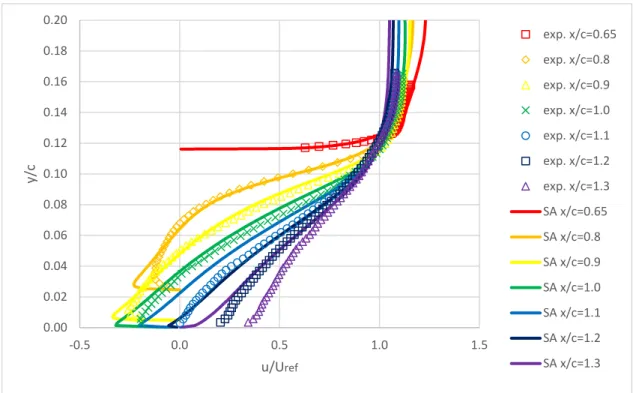
Figure 4.6 shows the comparison of computed pressure distribution obtained using the WA-DES model, WA model and SA model with the experimental data. Figure 4.7 shows the comparison of computed skin-friction distribution obtained using the same models and experimental data. It can be noted that the WA-DES model predicts the pressure distribution in most regions of the flow field quite well. From the skin friction distribution plot, it can be noted that the predicted separation occurs at x/c = 0.666 and reattachment at x/c = 1.12. These values are very close to the experimental data for separation and reattachment at 0.665 and 1.1 respectively. WA model and SA model over-predict the reattachment point at x/c = 1.4 and 1.3 respectively.

Figure 4.6: Comparison of pressure distribution on the surface of the hump.

-1.0 -0.8 -0.6 -0.4 -0.2 0.0 0.2 0.4 -0.5 0.0 0.5 1.0 1.5 2.0 Cp x/c exp. Cp WA-DES WA SA

(44)

25

Figure 4.7: Comparison of Skin-Friction distribution on the surface of the hump.

Comparisons of the predicted velocity profiles from WA-DES, WA and SA models and experimental data are shown in Figure 4.8, Figure 4.9 and Figure 4.10 respectively. It can be seen that the velocity profiles predicted by the WA-DES model agree quite well with the experimental data before and through the separation region. Downstream of the separation, recovery is slower than expected but it is still faster than that obtained with WA and SA models. Overall the results obtained using the WA-DES model are much more accurate than those obtained with conventional eddy-viscosity models [20].

-0.004 -0.002 0.000 0.002 0.004 0.006 0.008 -0.5 0.0 0.5 1.0 1.5 2.0 Cf x/c exp. Cf WA-DES WA SA

(45)

26

Figure 4.8: Comparison of velocity profiles from WA-DES model and experimental values at various locations on the hump.

Figure 4.9: Comparison of velocity profiles from WA model and experimental values at various locations on the hump. 0.00 0.02 0.04 0.06 0.08 0.10 0.12 0.14 0.16 0.18 0.20 -0.5 0.0 0.5 1.0 1.5 y/ c u/Uref exp. x/c=0.65 exp. x/c=0.8 exp. x/c=0.9 exp. x/c=1.0 exp. x/c=1.1 exp. x/c=1.2 exp. x/c=1.3 WA-DES x/c=0.65 WA-DES x/c=0.8 WA-DES x/c=0.9 WA-DES x/c=1.0 WA-DES x/c=1.1 WA-DES x/c=1.2 WA-DES x/c=1.3 0.00 0.02 0.04 0.06 0.08 0.10 0.12 0.14 0.16 0.18 0.20 -0.5 0.0 0.5 1.0 1.5 y/ c u/Uref exp. x/c=0.65 exp. x/c=0.8 exp. x/c=0.9 exp. x/c=1.0 exp. x/c=1.1 exp. x/c=1.2 exp. x/c=1.3 WA x/c=0.65 WA x/c=0.8 WA x/c=0.9 WA x/c=1.0 WA x/c=1.1 WA x/c=1.2 WA x/c=1.3

(46)

27

Figure 4.10: Comparison of velocity profiles from SA model and experimental values at various locations on the hump.

4.5.4 Flow over a Backward Facing Step

In flow over a backward facing step, a sudden back step is encountered by the flow resulting in flow separation. Figure 4.11 shows the geometry of the backward facing step and corresponding boundary conditions [20]. The Mach number at reference point (x/H = -4) is 0.128 and the Reynolds number based on the step height is 36,000. This is a typical benchmark case for testing the ability of the turbulence models in predicting flow separation.

0.00 0.02 0.04 0.06 0.08 0.10 0.12 0.14 0.16 0.18 0.20 -0.5 0.0 0.5 1.0 1.5 y/ c u/Uref exp. x/c=0.65 exp. x/c=0.8 exp. x/c=0.9 exp. x/c=1.0 exp. x/c=1.1 exp. x/c=1.2 exp. x/c=1.3 SA x/c=0.65 SA x/c=0.8 SA x/c=0.9 SA x/c=1.0 SA x/c=1.1 SA x/c=1.2 SA x/c=1.3

(47)

28

Figure 4.11: Geometry of backward facing step, computational domain and boundary conditions [20].

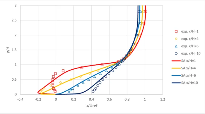
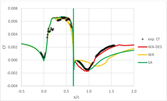
Figures 4.12 and 4.13 show the pressure distribution and skin friction coefficient respectively computed by the WA-DES model and their comparison with the experimental data. The

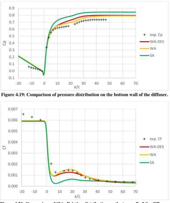
computed reattachment point is at x/H = 6.24 by WA-DES model compared to the experimental location range from 6.16 to 6.36. Pressure distribution and skin friction coefficient predicted by the WA-DES model generally match the experimental data, and show improved accuracy over WA model. Figures 4.14, 4.15 and 4.16 show the comparison of computed velocity profiles obtained using the WA-DES, WA and SA model with the experimental data, respectively. Velocity profiles from WA-DES and WA models at x/H = 1 and x/H = 4 are closer to the experimental results compared to the SA model, but the discrepancy between the computations and experimental data becomes larger when the flow approaches and moves beyond the

reattachment point (e.g. at x/H = 6 and 10). The WA-DES model generally gives the same results as the WA model; both show good agreement with the experimental data.

(48)

29

Figure 4.12: Comparison of pressure distribution on the surface of the backward facing step.

Figure 4.13: Comparison of Skin-Friction distribution on the surface of the backward facing step.

-0.3 -0.3 -0.2 -0.2 -0.1 -0.1 0.0 0.1 0.1 -5 0 5 10 15 20 25 30 Cp x/H exp. Cp WA-DES WA SA -0.002 -0.001 0.000 0.001 0.002 0.003 0.004 -5 0 5 10 15 20 25 30 Cf x/H exp. Cf WA-DES WA SA

(49)

30

Figure 4.14: Comparison of velocity profiles from WA-DES model and experimental values at various locations on the step.

Figure 4.15: Comparison of velocity profiles from WA model and experimental values at various locations on the step. 0 0.5 1 1.5 2 2.5 3 -0.4 -0.2 0 0.2 0.4 0.6 0.8 1 1.2 y/ H u/Uref exp. x/H=1 exp. x/H=4 exp. x/H=6 exp. x/H=10 WA-DES x/H=1 WA-DES x/H=4 WA-DES x/H=6 WA-DES x/H=10 0 0.5 1 1.5 2 2.5 3 -0.4 -0.2 0 0.2 0.4 0.6 0.8 1 1.2 y/ H u/Uref exp. x/H=1 exp. x/H=4 exp. x/H=6 exp. x/H=10 WA x/H=1 WA x/H=4 WA x/H=6 WA x/H=10

(50)

31

Figure 4.16: Comparison of velocity profiles from SA model and experimental values at various locations on the step.

4.5.5 Flow in an Asymmetric Plane Diffuser

Figure 4.17 shows the geometry of an asymmetric plane diffuser. Details of the geometry and boundary conditions are included in the NPARC Alliance CFD Verification and Validation Achieve (study #1) [23]. The inflow Mach number is 0.06 and the Reynolds number based on the inflow height H is ReH = 20,000 [24]. Adverse pressure gradient occurs on the inclined wall

which contributes to flow separation. WA-DES results are compared to the RANS results with WA and SA models and the experimental data for both the pressure coefficient and the skin friction distribution on the bottom wall and the top wall of the diffuser. Figures 4.18 and 4.19 show the comparison of pressure distribution on the top and bottom wall of the diffuser

respectively. Results of WA model best match the experimental data and the predictions of WA-DES model are slightly worse than that of the WA model. The computations from SA model have the poorest agreement with the experimental data among the three models. Figures 4.20 and 4.21 show the comparison of skin-friction distribution on the top and bottom wall of the diffuser

0 0.5 1 1.5 2 2.5 3 -0.4 -0.2 0 0.2 0.4 0.6 0.8 1 1.2 y/ H u/Uref exp. x/H=1 exp. x/H=4 exp. x/H=6 exp. x/H=10 SA x/H=1 SA x/H=4 SA x/H=6 SA x/H=10

(51)

32

respectively. As shown in Figure 4.20, WA-DES and WA models have good agreement with the experimental data for skin-friction on the top wall of the diffuser while SA model shows the poorest agreement. According to the experiment, the separation point occurs at x/H ≈ 6.6 and flow reattaches at x/H ≈ 27.5 on the top wall. In Figure 4.21, WA-DES model predicted

separation region on the bottom wall begins at x/H = 7.31 and ends at x/H = 26.13. This result is closer to the experimental value compared to that obtained using the WA and SA models, which predict the separation region on the bottom wall from x/H = 7.03 to 30.97 and x/H = 4.26 to 31.29, respectively.

Figure 4.17: Geometry of the asymmetric plane diffuser [23].

Figure 4.18: Comparison of pressure distribution on the top wall of the diffuser.

-0.1 0.0 0.1 0.2 0.3 0.4 0.5 0.6 0.7 0.8 0.9 -20 -10 0 10 20 30 40 50 60 70 Cp x/c exp. Cp WA-DES WA SA

(52)

33

Figure 4.19: Comparison of pressure distribution on the bottom wall of the diffuser.

Figure 4.20: Comparison of Skin-Friction distribution on the top wall of the diffuser.

-0.1 0.0 0.1 0.2 0.3 0.4 0.5 0.6 0.7 0.8 0.9 -20 -10 0 10 20 30 40 50 60 70 Cp x/c exp. Cp WA-DES WA SA 0.000 0.001 0.002 0.003 0.004 0.005 0.006 0.007 -20 -10 0 10 20 30 40 50 60 70 Cf x/c exp. Cf WA-DES WA SA

(53)

34

Figure 4.21: Comparison of Skin-Friction distribution on the bottom wall of the diffuser.

4.5.6 Flow past a NACA 4412 Airfoil

Subsonic flow past a NACA4412 airfoil is another benchmark test case used for evaluating the capability of the new WA-DES model. The freestream Mach number is 0.09 and the Reynolds number based on the Chord length is Re = 1.52 million. The angle of attack is 13.87 degrees. In the simulation, the outermost boundary of the computational domain is at a distance of 30 chords upstream from the leading edge of the airfoil. Surface pressure coefficient data and velocity profiles from the experiment of Coles et al. [25] are used to compare the simulations. No skin friction data is available, but the velocity profiles indicate that separation near the trailing edge occurs between x/c = 0.7 and 0.8. Computations using the WA-DES and WA model agree quite well with the experimental pressure coefficients, especially in the trailing edge region where separation occurs (x/c > 0.8) as shown in Figure 4.22 and Figure 4.23. However, SA model is unable to predict the separation region near the trailing edge accurately as shown in Figure 4.23. WA-DES, WA and SA model predict separation point at x/c = 0.76, 0.75 and 0.79, respectively.

-0.002 0.000 0.002 0.004 0.006 0.008 -20 -10 0 10 20 30 40 50 60 70 Cf x/c exp. Cf WA-DES WA SA

(54)

35

Figure 4.22: Comparison of pressure coefficient distribution on the surface of the NACA 4412 airfoil.

Figure 4.23: Zoomed-in-View of pressure coefficient distribution in the trailing edge separation region of NACA 4412 airfoil.

Figures 4.24, 4.25 and 4.26 compare the stream-wise velocity profiles at different locations on the airfoil surface. WA-DES computations show significant improvement in the results

compared to those from the WA model and the SA model in the separation region (x/c > 0.8) when compared to the experimental data. In the region before the separation point, the result of WA-DES model is better than that of the WA model but is worse than that of the SA model. Both WA-DES and WA models under-predict the magnitude of stream-wise velocities and the

-8.0 -7.0 -6.0 -5.0 -4.0 -3.0 -2.0 -1.0 0.0 1.0 2.0 0.0 0.2 0.4 0.6 0.8 1.0 Cp x/c exp. Cp WA-DES WA SA -2.0 -1.5 -1.0 -0.5 0.0 0.5 1.0 1.5 2.0 0.6 0.7 0.8 0.9 1.0 Cp x/c exp. Cp WA-DES WA SA