Overflow Juncture Flow Computations Compared with
Experimental Data
Henry C. Lee
⇤,
Science Technology Corporation, Moffett Field, CA 94035
Thomas H. Pulliam
†,
NASA Ames Research Center, Moffett Field, CA 94035
NASA’s Transformational Tools and Technologies Project (T3) is supporting a substantial effort to inves-tigate the formation and origin of separation bubbles found on wing-body juncture zones: the Juncture Flow experiment. The first phase of the Juncture Flow experiment, performed in NASA Langley’s 14- by 22-Foot Subsonic Tunnel, has been completed. This paper documents the CFD analysis done in conjunction with the experiment. Comparisons between CFD simulations and wind tunnel experimental results will be shown. Oil flow results, surface pressure cuts, velocity profiles, and Reynolds stress profiles will be compared. Preliminary results analyzing the effect of grid resolution, wind tunnel walls, and turbulence models on the above data will be presented. The results are not meant to be a validation study, but more as an evaluation of the current status of Reynolds averaged Navier Stokes (RANS) CFD simulations.
I. Introduction
Juncture flows are very difficult to predict, even with the current state-of-the-art CFD methods. In the AIAA drag prediction workshop 3 (DPW-3), which used the DLR-F6 wing-body, participants predicted a very wide range of side-of-body separations.1, 2 The same issue arose for the Common Research Model (CRM) in DPW-4 and DPW-5.3 The
introduction of the quadratic constitutive relation (QCR) by Spalart [4] did make the predicted separation bubble sizes over various CFD codes more homogeneous, but the solutions are still over-predicting bubble size when compared to experimental results.
There have been multiple experiments dedicated to juncture flow regions, most notable Simpson [5] and Gand et al. [6] with the ONERA group, but very few were able to obtain measurements in the trailing-edge corner separation, on a swept wing configuration. Simpson’s work focused more on the leading edge horseshoe vortex, while ONERA’s experiment was an unswept wall-mounted wing.
NASA, through its Transformational Tools and Technologies Project (T3) under Transformative Aeronautics
Con-cepts Program (TACP), is supporting a substantial effort, the Juncture Flow (JF) experiment, to investigate the forma-tion and origin of separaforma-tion bubbles found on wing-body juncture zones. The experiment is intended to be primarily for the purpose of CFD validation and turbulence model development for wing-juncture trailing edge separation onset and progression. The committee members decided upon a sting-mounted swept-wing and fuselage model, with a Laser Doppler velocimetry (LDV) system inside the fuselage (as opposed to the traditional LDV system mounted behind the wind tunnel walls). The goal was to observe the onset and growth of the separation bubble in aft juncture flow region of a realistic wing-body configuration. Placing the LDV system inside the fuselage provides a way to measure the leading-edge and trailing-edge juncture regions. The Juncture Flow Model (JFM) is a reduced scale model, i.e. 8%, based on the full scale CRM.
A campaign of risk reduction experiments, and accompanying CFD simulations, including: 1. Fluid Mechanics Lab (FML) Test Cell 2 at NASA Ames Research Center 3% semispan model7
2. Virginia Tech Stability Tunnel 2.5% model8
3. NASA Langley 14-by-22 Ft. Subsonic Wind Tunnel 6% model9
helped finalize the experiment design and maximize the value of the data obtained in the final tests. The JF team settled on two different interchangeable wing configurations, including a wing based on a DLR-F6 wing and a NACA
⇤Member AIAA, Research Scientist,Computational Aerosciences Branch, ARC, MS 258-2
†Associate Fellow, AIAA, Senior Research Scientist, Computational Aerosciences Branch, ARC, MS 258-2
based wing, for the final test. Only the former wing was tested in the wind tunnel campaign performed in late 2017 and early 2019.
Experimental data and Overflow CFD data will be presented. Data including oil flow results, surface pressure cuts, Reynolds stress profiles, and velocity profiles will be compared. Preliminary results pertaining to CFD sensitivity to parameters including grid resolutions, turbulence models, and wall effects will be explored. Further details on the experimental setup and results can be found in a companion paper by Kegerise et al. [10], and further CFD comparisons can be found in Rumsey et al. [11].
This paper is not meant to serve as a validation of the CFD solvers, but more so as an evaluation of the current state of CFD simulations. The experiment was designed using CFD analysis, and now that experimental data is available, we would like to assess how well the CFD simulations performed.
II. 14-by-22 Foot Subsonic Wind Tunnel JFM Experiment
The JFM experiment was performed in the 14-by-22 Ft. Subsonic Tunnel (14x22), and the full results can be found in Kegerise et al. [10]. A very brief description of the relevant experimental setup will be presented below. The subsequent subsections will discuss the 14x22 wind tunnel and the Juncture Flow Model.
A. 14 -by-22 Ft. Subsonic Wind Tunnel
The experiment was performed in the Langley 14-by-22 Ft. Subsonic Tunnel (14x22), which is a closed-circuit, atmospheric-pressure wind tunnel. This test was made in the closed test section mode, which results in a 14.5 ft high and 21.75 ft wide test section. Figure 1a shows the full circuit of the 14x22 with the high speed leg outlined in blue, and 1b describes the sections of the high speed leg.
(a) 14x22 with high speed leg highlighted (b) Sections of high speed leg
Figure 1. 14x22 Wind Tunnel, High Speed Leg
Further details about the tunnel can be found in Gentry et al. [12]. The flow condition of primary interest for this experiment wasRec= 2.4million.
B. Juncture Flow Model
The Juncture Flow Model is a large aluminum model consisting of a fuselage and a number of interchangeable wing candidates. The model wing span was nominally 3397.250 mm, fuselage length was 4839.233 mm, and crank chord (the chord at the y-station with trailing edge break) was 557.17 mm. The fuselage nose is atx= 0mm, the x-axis was aligned with the fuselage centerline, the y-axis ran starboard, and the z-axis was up. The fuselage side wall is planar over much of the body (to make it easier to install windows for the laser-based measurement systems), at
y= 236.1mm. The F6 wing leading edge horn is located nearx= 1925.0mmat the fuselage, while the F6 wing root
trailing edge is located atx= 2961.9mm. The fuselage housed two separate LDV systems, mounted on a traverse
edge. The wings are designed to have removable leading edge horns. This paper will focus on the model with the leading edge horn installed, which has the largest experimental dataset. Further information of the experiment setup can be found in Kegerise et al. [10]. Figure 2 details the parts on the JFM.
Figure 2. Juncture Flow Model Parts.
III. Computational Fluid Dynamics, Overflow
CFD solutions are performed with Overflow. Simulations are run in air, first, and then with the wind tunnel walls, to assess the wall effects. The subsequent sections will cover how the Overflow simulations are set up.
A. Overflow Setup
A series of overset grids were created for the Juncture Flow Model. There is a commonality between the grids used in all of the CFD simulations. The grids are built using Chimera Grid Tools.13 The full span JFM configuration consists
of a fuselage, and two wings. The fuselage is built from 4 zones, two of which span the length of the fuselage, and two cap grids covering the nose and rear of the fuselage. The wing grids for all the various configurations share a common 6 zone topology. The wing grids consist of two collar grids covering the wing-fuselage junction, two grids spanning the wing, and two wing tip cap grids. Each pair of grids have overlap along the chord, making effectively a front and rear zone. All the surface grids are projected back to the reference CAD geometry using Pointwise14to
ensure a smooth surface geometry.
For the free air grids, a series of grids with increasing grid resolution are built. Four grid topologies, including a coarse, medium, fine, and extra-fine grid, were constructed. Figure 3 shows the grid density on the surface of the port wing and fuselage, as well as a zoomed in view of the root-trailing edge region. The overall vehicle includes 16 grid zones, and Table 1 details the various configurations looked at in this study, and the grid metrics for each configuration. The near body grid point counts include just the volume grids for the JFM, excluding the support hardware, and applicable wind tunnel or off-body Cartesian grids.
Table 1. Overflow Grid Summary
Configuration Max Stretching Ratio Near Body Grid Points Total Grid Points
Air Coarse 1.20 19,370,462 21,374,660
Air Medium 1.15 47,580,599 49,726,586
Air Fine 1.10 163,552,251 165,714,572
Air Extra Fine 1.08 382,086,347 398,391,568 Wind Tunnel Medium 1.15 47,580,599 92,582,251 Wind Tunnel Fine 1.10 163,552,251 325,462,526
(a) Coarse (b) Coarse TE region
(c) Medium (d) Medium TE Region
(e) Fine (f) Fine TE Region
(g) Extra Fine (h) Extra Fine TE Region 4 of 43
For all the free air cases, the JFM grids are embedded in Overflow’s off-body Cartesian grid system. Domain connectivity is performed using Overflow’s object x-rays.15 The far-field domain is set to be 100 chord lengths away.
The free air simulations are run at Mach numberM1 = 0.189atT = 529Rankine, with a Reynolds number of 2.4
million based on the yehudi break chord. The free air simulations are run at an uncorrected angle of attack of 2.5
and5.0 . Theoretically, there should be an angle of attack correction to account for the wall effects, but this data was unavailable at the time of the test.
All of the Overflow cases are run with Overflow 2.2N. The3rd-order Roe upwind scheme16is used for the
convec-tive fluxes, and the implicit solve was done using ARC3D Beam-Warming scalar pentadiagonal scheme and low-Mach preconditioning.17 The Spalart-Allmaras turbulence model with the rotational correction (RC) and QCR201318is used
for most of the cases. All the cases were run fully turbulent. Additional cases looking at turbulence model effects on the juncture flow region will be explored later in Section IV.C. The effect of not using QCR, as well as using the SST turbulence model with the rotational correction and QCR will be compared.19, 20 In short, solutions with three
turbulence models:
1. SA-Noft2-RC-QCR2013 (SARC-QCR)18
2. SA-Noft2-RC (SARC)21
3. SST-RC-QCR2013 (SSTRC-QCR)20
will be presented. The CFD free air (CFD air) results are computed using 420 Intel Broadwell cores, and utilized approximately 12 hours of walltime.
For the wind tunnel grids, wall grids are built from the as-built laser scanned CAD as specified in Nayani et al. [22]. Fifteen zones modeled the high-speed leg of the 14x22. The tunnel is split into five sections streamwise: plenum, test section, diffuser part 1, diffuser part 2, and extended diffuser. Each section was comprised of two viscous wall grids, and one core grid. The average grid spacing is varied to produce a medium (0.5 ft., 152.4 mm), and fine (0.25 ft., 76.2 mm) grid. Minimum spacing at the walls of the test section is less than 0.00001 ft. (0.003048mm) on all grids. The straight section of the inlet, prior to the contraction, is run with inviscid walls. The diffuser grids gradually coarsened downstream. A diffuser extension of 100 ft. (30,480 mm) streamwise is incorporated, and the extended diffuser walls also use an inviscid boundary condition. Figure 4 shows the wind tunnel volume grid with the extended diffuser, and an overall view of the 14x22 with the JFM installed. Utilizing inviscid spans of the tunnel help increase the code stability at the boundary conditions, and help accelerate the convergence of the CFD code. The details and benefits of using this method can be found in by Lee et al. [23]. Domain connectivity and hole cutting was performed using Overflow’s object xrays as well.15
The JFM installation location for both↵= 5.0 and↵= 2.5 cases was based on CAD. Different geometries
were necessary for the two angles of attack, as the mast on the support did change to place the model in the center of the tunnel. Figure 5 shows a zoomed in region of the test section with the JFM installed at both angles of attack. There is a slight variation of the angle of attack (±0.05 ) throughout the test that the CFD does not account for. For
the wind tunnel results shown below, the free air medium and fine grids were embedded directly into the wind tunnel configuration for consistency between and free air and tunnel calculations.
The wind tunnel with the JFM installed (at their respective angles of attack) were translated and rotated to match the same coordinate system as the free air grid system (body coordinate system), to greatly simplify the post processing. In doing this, all the flow quantities, velocities, etc. from a post processing standpoint, were already in the JFM body coordinate system as opposed to the tunnel coordinate system. This eliminates the need to transform the flow data to the body coordinate system when post processing the data.
(a) Volume grid of 14x22 Wind Tunnel. (b) Juncture Flow Model grid installed in high speed leg of 14x22.
(a) Juncture Flow Model in 14x22 at↵= 5.0 . (b) Juncture Flow Model in 14x22 at↵= 2.5 .
Figure 5. Juncture Flow Model as installed in the 14x22 Foot Subsonic Wind Tunnel.
In the 14x22 wind tunnel, the Reynolds number is held constant at 2.4 million (±0.3%) based on the crank cord.
Throughout the testing, the atmospheric conditions did change, resulting in a spread of Mach numbers ranging from 0.175 to 0.205, temperatures ranging from 495 to 554.4 Rankine (275 308 K), and dynamic pressures ranging from 2107 to 2921 Pa. Median values were chosen for the CFD air runs, and they correspond toM1 = 0.189, and
T = 519.912Rankine.
The wind tunnel also is modeled using the same chosenM1 = 0.189, a reference temperature ofT = 519.912
Rankine (T = 299.94K), and a Reynolds number of 2.4 Million based on the yehudi break chord. Stagnation temper-ature and stagnation pressure based on a reference condition ofM1 = 0.189are imposed at the inlet boundary, and
a back pressure ratio is specified at the tunnel exit. A combination of the static and stagnation pressure measurements are used to calculate the tunnel speed, and the back pressure was iterated until the wind tunnel reached the desired conditions. More on this method of simulating the wind tunnel can be found in Lee et al. [23].
The CFD wind tunnel (CFD wind tunnel) simulations used 800 Intel Skylake Cores, for anywhere between 60 to 120 hours of walltime. The wind tunnel simulations take a lot longer to run, due to the need to iterate the back pressure to get the tunnel conditions to match. Using a proportionalintegralderivative controller (PID)24 to drive the
correct back pressure did help, but still requires a considerable run time. Table 1 outlines the JFM number of grid points and total number of grid points for each of the CFD wind tunnel cases.
IV. Results
The Overflow computational simulations will be compared with experimental results.10 Side-of-body bubble
sep-aration sepsep-aration widths, pressure coefficient (CP), velocity and Reynolds stress plots and profiles will be presented. CFD solutions, in air and with wind tunnel wall, with varying grid resolutions will be presented. Variations in tur-bulence models (in air) will also be shown. The larger number of results presented here are free air computations which is the typical mode of operation for CFD studies. Free air computations converge faster than the wind tunnel calculations, due in part to the need to calibrate each run in the wind tunnel for a consistent Mach number incoming to the model, and also due to the smaller grid requirements. As will be shown below, in most cases the free air results and wind tunnel results are consistent, sometimes for specific quantities, (e.g. pressure distributions away from the juncture flow region and wing tip), and even when not comparable in certain regions, the trends are consistent.
Figure 6 shows a representative side of body separation width and length for ↵ = 5.0 and↵ = 2.5 , and
indicate that data was taken from the CFD computation (surface streamlines) by finding a dividing particle trace line from the separation inception and using that to define length and maximum width. Note that there is a fair amount of arbitrariness to the extracted values. Velocity profiles and Reynolds stresses from both the LDV data and CFD extractions will be shown. Experimental data will always be plotted in black, with uncertainties representing a 95% confidence interval (2 ) when available.
Figures 7 and 8 show the separation bubble size as a function of near body grid density, for all the cases at↵= 5.0
and↵ = 2.5 . The experimental values with uncertainties are shown along the vertical axis. The CFD Air cases all over-predict the bubble size, when compared to the experimental values. Sweeps were run with three different turbulence models, and will be further discussed Section IV.C. SARC predicted the largest bubble sizes, followed by SSTRC-QCR, and lastly SARC-QCR. The cases run with wind tunnel walls also predicted smaller bubble sizes than their similar air case. The cases with the wind tunnel walls also seem to extrapolate to the experimental data values.
Figures 9 and 10 show coefficient of pressure slices at various stations on the model, for all the cases run (with SARC-QCR). Note that experimental surface pressure data from the test have not been fully processed as of the time
(a) Side-of-body separation example↵= 5.0 (b) Side-of-body separation example↵= 2.5
Figure 6. Typical side-of-body separation, CFD surface streamlines.
(a) Separation length at↵= 5.0 (b) Separation width at↵= 5.0
Figure 7. Separation size as a function of grid density and turbulence model↵= 5.0 .
(a) Separation length at↵= 2.5 (b) Separation width at↵= 2.5
of this writing. Therefore, theseCPcomparisons should be considered preliminary. For the↵= 5.0 case, most of the differences are at the leading edge, at the juncture flow region in the separation bubble, and at the wing tip. Higher grid densities lead towards a higher peak in pressure on the leading edge. Results are shown for the free air grid refinement compared with the wind tunnel medium and fine grid cases. The JFM grids are the same between the free air to wind tunnel sting-mast (WT+ST) medium and fine cases. Tip loading seems to be increased as the grids refine, due to the increased resolution of the wing tip vortex and it’s influence on tip loading. The CFD↵= 5.0 cases with the wind tunnel walls seem to have higher peaks than the free air case. Similarity, the CFD↵= 2.5 cases with wind tun-nel walls show differences on the pressure side of the wing. Both can probably be attributed to wind tuntun-nel wall effects.
(a) WingCPcuts locations (b)y= 254mm (c)y= 290.83mm
(d)y= 482.6mm (e)y= 685.8mm (f)y= 994.92mm
(g)y= 1295.4mm (h)y= 1663.7mm (i)x= 2667.0mm
(a) WingCPcuts locations (b)y= 254mm (c)y= 290.83mm
(d)y= 482.6mm (e)y= 685.8mm (f)y= 994.92mm
(g)y= 1295.4mm (h)y= 1663.7mm (i)x= 2667.0mm
Figure 10. CPslices for↵= 2.5 for all CFD grids (SARC-QCR).
A. CFD Free Air Grid Sequence Comparisons
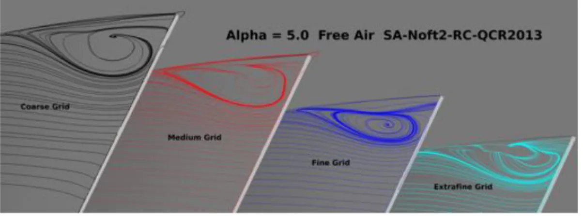
A series of grid levels, including a coarse, medium, fine, and extra-fine were run. For brevity, only the results run with SARC-QCR will be shown here. Figures 11 and 12 show the corresponding side of body separation bubble topology for the 4 levels of grid refinement. The size of the bubble seems very similar in the fine and extrafine cases, yet the surface streamlines are different, suggesting that the flow is very much three dimensional.
Figures 13 and 14 show slice contours of velocity and Reynolds stresses in the trailing edge region for the medium and fine grid. These slices also correspond approximately to the regions where the LDV data were taken. The three dimensional bubble size for the medium grid looks slightly larger than the fine grid.
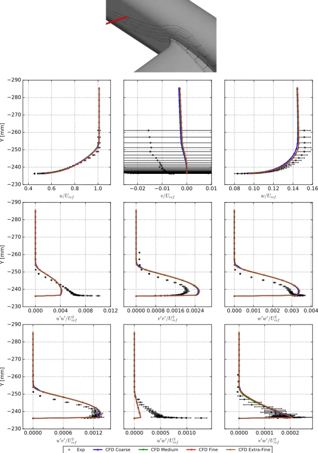
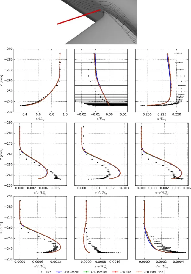
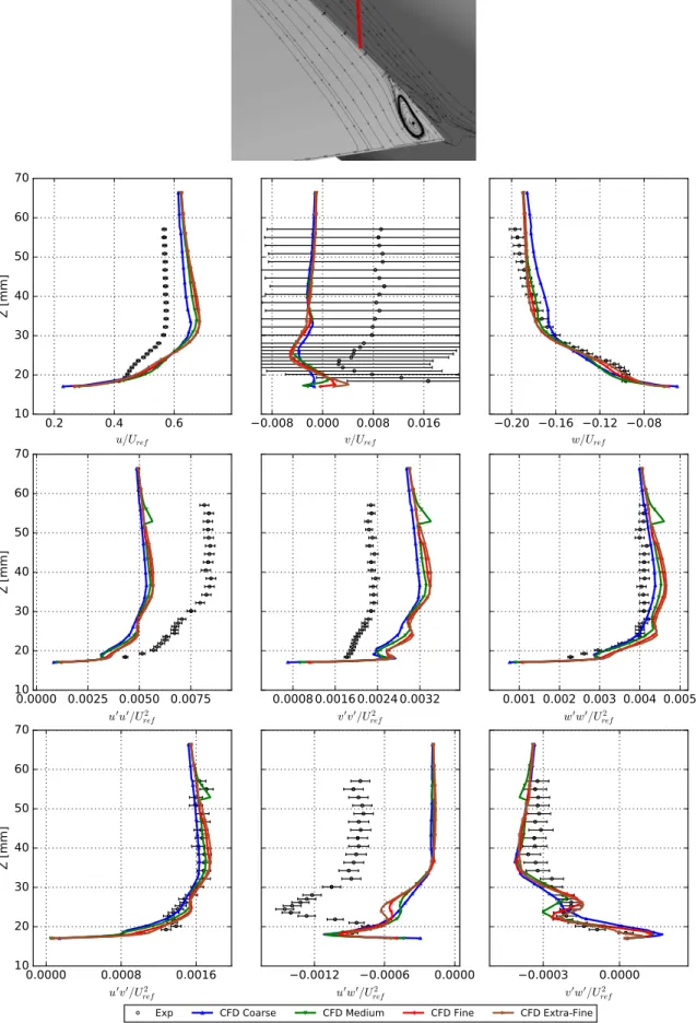
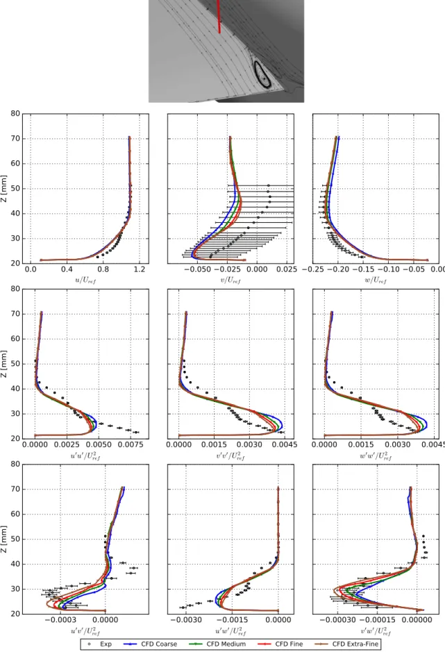
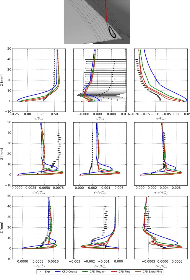
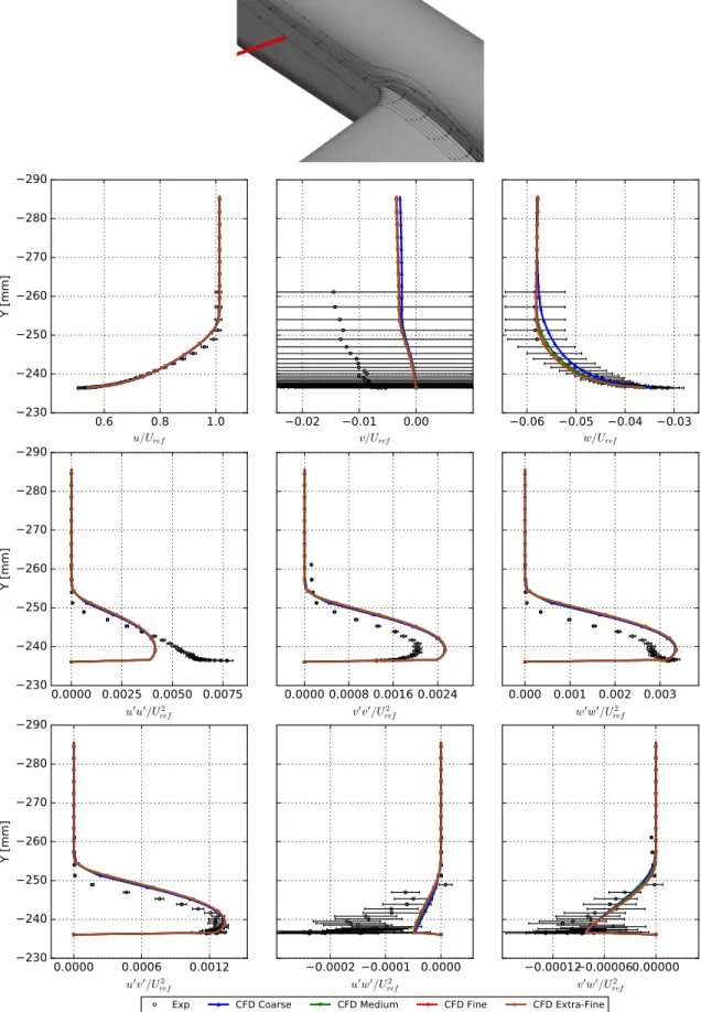
Comparisons between the experimental LDV measurements and CFD (grid refinement air cases) extracted veloci-ties and Reynolds stresses are shown in Figs. 15 to 20 for↵= 5.0 , and Figs. 21 to 26 for↵= 2.5 . The top picture in each figure shows CFD surface streamlines highlighting the juncture flow region, and the red line represents the extracted profile line. The velocities in the regions leading up to the separation bubble agree very well with the LDV
Figure 11. Side of body separation bubble topology vs grid refinement↵= 5.0 .
Figure 12. Side of body separation bubble topology vs grid refinement↵= 2.5 .
data. There is almost no variation due to grid resolution, for the velocities and Reynolds stresses, with the exception of the coarse grid, which stands out versus the rest of the finer grids.
Reynolds stresses do compare fairly well in regions upstream of the separation bubble. Notably,v0v0seems to be
over-predicted at all the grid resolutions, whileu0w0 is both under-predicted and over-predicted. The values ofu0u0
are under-predicted in the regions upstream of the separation bubble, as seen in Fig. 17 and Fig. 23, yetu0u0 does
match better away from the wall just30mmaway from the fuselage, in Fig. 18 and Fig. 24.
Figure 19 and Fig. 25 are both located close to the start of the separation. Both show that the CFD is starting to predict some form of separation, contrary to the experiment. The velocities and Reynolds stresses show no signs of correlation in Fig. 20 and Fig. 26, often over-predicting the experiment in magnitude in the separation region. The reverse flow region seems to get closer to the wing surface as the grid resolution increases, though this trend stops around the fine grid level.
Figure 15. Grid Refinement Comparison (CFD Air): Velocities and Reynolds Stresses at↵= 5.0 , x= 1168.4, z= 0.0, just past nose of
Figure 16. Grid Refinement Comparison (CFD Air): Velocities and Reynolds Stresses at↵= 5.0 , x= 1859.2, z= 55.05, just upstream of the LE.
Figure 17. Grid Refinement Comparison (CFD Air): Velocities and Reynolds Stresses at↵= 5.0 , x= 2747.6, y= 237.1, upstream of separation, 1 mm from fuselage.
Figure 18. Grid Refinement Comparison (CFD Air): Velocities and Reynolds Stresses at↵= 5.0 , x= 2747.6, y= 266.1, upstream of separation, 30 mm from fuselage.
Figure 19. Grid Refinement Comparison (CFD Air): Velocities and Reynolds Stresses at↵= 5.0 , x= 2822.6, y= 237.1, close to start
Figure 20. Grid Refinement Comparison (CFD Air): Velocities and Reynolds Stresses at↵ = 5.0 , x = 2892.6, y = 246.1, in the
Figure 21. Grid Refinement Comparison (CFD Air): Velocities and Reynolds Stresses at↵= 2.5 , x= 1168.4, z= 0.0, just past nose
Figure 22. Grid Refinement Comparison (CFD Air): Velocities and Reynolds Stresses at↵= 2.5 , x= 1859.2, z= 55.05, just upstream of LE.
Figure 23. Grid Refinement Comparison (CFD Air): Velocities and Reynolds Stresses at↵= 2.5 , x= 2757.6, y= 237.1, upstream of separation, 1 mm from fuselage.
Figure 24. Grid Refinement Comparison (CFD Air): Velocities and Reynolds Stresses at↵= 2.5 , x= 2757.6, y= 266.1, upstream of separation, 30 mm from fuselage.
Figure 25. Grid Refinement Comparison (CFD Air): Velocities and Reynolds Stresses at↵= 2.5 , x= 2869.6, y= 237.1, upstream of
Figure 26. Grid Refinement Comparison (CFD Air): Velocities and Reynolds Stresses at↵= 2.5 , x= 2899.6, y= 246.1, at the start
B. CFD Wind Tunnel Wall Effects
A preliminary investigation of the wind tunnel wall effect on the juncture flow region is covered in this section. The exact same near body grids used in the CFD air medium and fine grid simulations are used and embedded into the 14x22 wind tunnel. The hope is that using the same near body grids can help isolate some of the wind tunnel modeling effects on the juncture flow region. An effort was made to keep the spacing similar in the test section, as the CFD air cases, but the 14x22 tunnel grids are still going to be inherently finer, due to how the grids were constructed.
Figure 27 shows the separation topology for both the CFD air and CFD wind tunnel cases. The overall shape of the bubble for the same grid resolution is very similar. The medium grids show a larger bubble size than the fine grids, and the CFD air cases present a larger bubble size than the CFD wind tunnel simulations.
(a) Bubble topology for↵= 5.0
Figure 27. Side of body separation bubble topology, tunnel wall effect.
The contour plots of the velocities and Reynolds stresses in Figs 28 and 29 give a three dimensional picture of the bubble. The contours between the medium and fine grid are very similar. However, when compared to the free air case, Figs. 13 and 14, there are more differences. The bubble seems to be taller and slightly narrower in the wind tunnel, while shorter and wider in the corresponding air case. There are still many similarities throughout the contours. Figures 30 to 35 show the velocity and Reynolds stress profiles for the air medium, air fine, wind tunnel medium, and wind tunnel fine grids. Overall, the CFD wind tunnel profiles are very similar to each other, while the CFD air results show a little more spread.
The profiles are nearly identical upstream of the wing, in Figs. 30 and 31, with only thewprofile being different.
The speed in thewdirection is higher in the wind tunnel, and agrees with the experiment as well. Figures 32 and
33 show the profiles upstream of the separation on the wing. The velocity profiles are still very similar, while the Reynolds stress profiles are starting to differ between the CFD air and CFD wind tunnel. At the start of separation, in Fig. 34, the profiles start to differ greatly between the CFD air and CFD wind tunnel. The CFD wind tunnel cases only predict a slight separation, while the CFD air profiles show a separation. In the separation bubble, in Fig. 35, the velocity profiles for the CFD wind tunnel show good agreement with the experimental data. The Reynolds normal stress profiles do look similar, with larger magnitudes for the CFD air cases, but are much larger than the experimental data. Only thev0w0Reynolds shear stress compare well with each other.
Figure 32. Tunnel Wall Effect Comparison Velocities and Reynolds Stresses at↵= 5.0 , x= 2747.6, y= 237.1, upstream of separation, 1 mm from fuselage.
Figure 33. Tunnel Wall Effect Comparison Velocities and Reynolds Stresses at↵= 5.0 , x= 2747.6, y= 266.1, upstream of separation, 30 mm from fuselage.
Figure 34. Tunnel Wall Effect Comparison Velocities and Reynolds Stresses at↵ = 5.0 , x = 2822.6, y = 237.1, close to start of
C. CFD Turbulence Model Comparison
The effect of different turbulence models, including: 1. SA-Noft2-RC-QCR2013 (SARC-QCR) 2. SA-Noft2-RC (SARC)
3. SST-RC-QCR2013 (SSTRC-QCR)
on the juncture flow region, are explored in this section. While all the grid resolutions were run with the three turbulence models, results only on the fine grid at↵ = 5.0 will be shown,for brevity. Additional results will be available on the Turbulence Modeling Resource website [25].
Figure 36 shows the separation bubble topology for the various turbulence models runs. Both SARC and SSTRC-QCR predict a larger bubble size than SARC-SSTRC-QCR.
Figure 36. Side of body separation bubble topology vs turbulence model↵= 5.0 .
Figure 37 shows theCP slices at various stations. Overall, the pressures are very similar throughout most of the flow, with the largest differences occurring at the leading edge peaks, the separation zones, and the wing tips.
Comparisons between the velocity profiles and Reynolds stress profiles are shown in Figs. 38 through 43. It is hard to say which model performs best overall, as they all trade off. SSTRC-QCR seems to better match the experiment’s Reynolds stresses, in Figs. 38 and 39, yet miss on thewcomponent of velocity. SARC in the nose and leading edge region over-predicts some Reynolds stresses, and under-predicts others.
Near the trailing edge, in Figs. 40 and 41, SSTRC-QCR seems to have a different profile than the SA-based turbulence models. The SA models generally have a similar profile. However, at the start of the separation, Fig. 42, the SSTRC-QCR and SARC models have predicted separation, while the SARC-QCR model has not. From the earlier bubble size measurements, both the SSTRC-QCR and SARC models over-predicted the separation size across all the grids, and the profiles here show that as well. There is almost no correlation to the profiles in the separation bubble, in Fig. 43, between the turbulence models. Further examination of this data is needed, to fully understand how each turbulence model is affecting the juncture flow.
(a) WingCPcuts locations (b)y= 254mm (c)y= 290.83mm
(d)y= 482.6mm (e)y= 685.8mm (f)y= 994.92mm
(g)y= 1295.4mm (h)y= 1663.7mm (i)x= 2667.0mm
Figure 40. Turbulence Model Comparison: Velocities and Reynolds Stresses at↵= 5.0 , x= 2747.6, y= 237.1, upstream of separation, 1 mm from fuselage.
Figure 41. Turbulence Model Comparison: Velocities and Reynolds Stresses at↵= 5.0 , x= 2747.6, y= 266.1, upstream of separation, 30 mm from fuselage.
Figure 42. Turbulence Model Comparison: Velocities and Reynolds Stresses at↵ = 5.0 , x = 2822.6, y = 237.1, close to start of
V. Conclusions
A series of CFD cases were run with Overflow as a companion to the first phase of the Juncture Flow Model experiment. The recent experiment10 provides detailed flowfield data in the wing-body junction (corner) region near
the wing trailing edge where separation occurs. Preliminary CFD data was compared with experimental data, exploring where the current state of RANS CFD simulations lies. Juncture flow sensitivity to grid resolution, turbulence model, and tunnel walls was presented.
The data presented in this paper provides a preliminary look at how well (or poorly) today’s state-of-the-art RANS CFD simulations perform. No specific judgments or assessments of the results based on comparisons with the experi-mental data have been made. It is expected that there will be differences, sometimes small and other-times significant. The purpose of this overall project is to provide data for improvements of Reynolds averaged turbulence models, assessment and development of LES and higher order turbulence models, and also provide validation data.
Interested readers are referred to the experimental papers, Kegerise et al. [10], Jekins et al. [26] and the com-panion paper, Rumsey et al. [11]. An extensive NASA report on the experiment is forthcoming and future test are being planned. The experimental configuration, conditions and computational data will be eventually available on the Turbulence Modeling Resource website [25].
Acknowledgments
The authors would like to thank the NASA Transformational Tools and Technologies Project for support of the research presented in this paper. The authors would also like to thank the Juncture Flow Committee members, and Chris Rumsey for leading the Juncture Flow Experiment.
References
1Sclafani, A. J., Vassberg, J. C., Harrison, A. N., Rumsey, C. L., Rivers, S. M., and Morrison, J. H., “CFL3D/OVERFLOW Results for DLR-F6 Wing/Body and Drag Prediction Workshop Wing,”Journal of Aircraft, Vol. 45, No. 3, 2008, pp. 762–780.
2Vassberg, J., Tinoco, E., Mani, M., Brodersen, O., Eisfeld, B., Wahls, R., Morrison, J., Zickuhr, T., Laflin, K., and Mavriplis, D., “Abridged Summary of the Third AIAA Computational Fluid Dynamics Drag Prediction Workshop,”AIAA Journal of Aircraft, Vol. 45, No. 3, 2008, pp. 781– 798.
3Levy, D., Laflin, K., Tinoco, E., Vassberg, J., Mani, M., Rider, B., Wahls, C. R. R., Morrison, J., Broderson, O., Crippa, S., Mavriplis, D., and Murayama, M., “Summary of Data from the Fifth Computational Fluid Dynamics Drag Prediction Workshop,”Journal of Aircraft, Vol. 51, No. 4, 2014, pp. 1194–1213.
4Spalart, P. R., “Strategies for Turbulence Modelling and Simulation,”International Journal of Heat and Fluid Flow, Vol. 21, 2000, pp. 252– 263.
5Simpson, R. L., “Juncture Flows,”Annual Review of Fluid Mechanics, Vol. 33, 2001, pp. 415–443.
6Gand, F., Deck, S., and Brunet, V., “Flow Dynamics Past a Simplified Wing Body Junction,”Physics of Fluids, Vol. 22, No. 11, Nov. 2010, pp. 11511.
7Roozeboom, N. H., Lee, H. C., Zilliac, G. G., and Pulliam, T. H., “Comparison of Experimental Surface and Flow Field Measurements to Computational Results of the Juncture Flow Model,” AIAA Paper 2016-1558, Jan. 2016.
8Rumsey, C., Neuhart, D., and Kegerise, M., “The NASA Juncture Flow Experiment: Goals, Progress, and Preliminary Testing,” AIAA Paper 2016–1557, January 2016.
9Lee, H. C., Pulliam, T. H., Neuhart, D., and Kegerise, M. A., “CFD Analysis in Advance of the NASA Juncture Flow Experiment,” AIAA Paper 2017-4127, 2017.
10Kegerise, M., Neuhart, D., Hannon, J., and Rumsey, C., “An Experimental Investigation of a Wing-Fuselage Junction Model in the NASA Langley 14- by 22-Foot Subsonic Wind Tunnel,” To be presented at AIAA SciTech Meeting FD-04: Special Session: CFD 2030 - Experiments and Computations for Juncture Flows, San Diego, CA, January 2019.
11Rumsey, C., Carlson, J., and Ahmad, N., “FUN3D Juncture Flow Computations Compared with Experimental Data,” To be presented at AIAA SciTech Meeting FD-04: Special Session: CFD 2030 - Experiments and Computations for Juncture Flows, San Diego, CA, January 2019.
12Gentry Jr, C. L., Quinto, P., Gatlin, G., and Applin, Z., “The Langley 14- by 22-Foot Subsonic Tunnel: Description, Flow Characteristics, and Guide for Users,” NASA TP–3008, September 1990.
13Chan, W. M., Gomez, R. J., Rogers, S. E., and Buning, P. G., “Best Practices in Overset theGrid Generation,” AIAA Paper 2002-3191, Jun. 2002.
14“User’s Manual, Pointwise V18,”https://www.pointwise.com/doc/user-manual/, Accessed: 2018-09-27. 15Meakin, R. L., “Object X-Rays for Cutting Holes in Composite Overset Structured Grids,” AIAA Paper 2001–2537, June 2001. 16Roe, P. L., “Approximate Riemann Solvers, Parameter Vectors, and Difference Schemes,”J. Comp. Phys., Vol. 43, 1981, pp. 357–372. 17Nichols, R. H. and Buning, P. G., “User’s Manual for Overflow 2.2,” http://overflow.larc.nasa.gov/home/ users-manual-for-overflow-2-2/, Accessed: 2017-03-15.
18Mani, M., Babcock, D., Winkler, C., and Spalart, P., “Predictions of a Supersonic Turbulent Flow in a Square Duct,” AIAA Paper 2013–0860, January 2013.
20Smirnov, P. E. and Menter, F. R., “Sensitization of the SST Turbulence Model to Rotation and Curvature by Applying the Spalart-Shur Correction Term,” Vol. 131, No. 041010, 2009.
21Shur, M. L., Strelets, M. K., Travin, A. K., and Spalart, P. R., “Turbulence Modeling in Rotating and Curved Channels: Assessing the Spalart-Shur Correction,”AIAA Journal, Vol. 38, No. 5, 2000, pp. 784–792.
22Nayani, S. N., Sellers, W., Tinetti, A. F., Brynildsen, S. E., and Walker, E. L., “Numerical Simulation of a Complete Low-Speed Wind Tunnel Circuit,” AIAA Paper 2016–2117, January 2016.
23Lee, H. C., Pulliam, T. H., Rumsey, C. L., and Carlson, J. R., “Simulations of the NASA Langley 14- by 22-Foot Subsonic Tunnel for the Juncture Flow Experiment,” 2018.
24Carlson, J., “Automated Boundary Conditions for Wind Tunnel Simulations,” NASA TM 2018-219812, 2018. 25http://turbmodels.larc.nasa.gov, Accessed: 2017-03-21.
26Jenkins, L., Yao, C.-S., and Bartram, S., “Flow-Field Measurements in a Wing-Fuselage Junction Using an Embedded Particle Image Velocimetry System,” To be presented at AIAA SciTech Meeting FD-04: Special Session: CFD 2030 - Experiments and Computations for Juncture Flows, San Diego, CA, January 2019.