Three-dimensional numerical analysis of flow structure and sediment transport process in open channels

Three-dimensional numerical

analysis of flow structure and

sediment transport process in

open channels

Esteban Sánchez Cordero

ADVERTIMENT La consulta d’aquesta tesi queda condicionada a l’acceptació de les següents condicions d'ús: La difusió d’aquesta tesi per mitjà del r e p o s i t o r i i n s t i t u c i o n a l UPCommons (http://upcommons.upc.edu/tesis) i el repositori cooperatiu TDX

( h t t p : / / w w w . t d x . c a t / ) ha estat autoritzada pels titulars dels drets de propietat intel·lectual

únicament per a usos privats emmarcats en activitats d’investigació i docència. No s’autoritza la seva reproducció amb finalitats de lucre ni la seva difusió i posada a disposició des d’un lloc aliè al servei UPCommons o TDX. No s’autoritza la presentació del seu contingut en una finestra o marc aliè a UPCommons (framing). Aquesta reserva de drets afecta tant al resum de presentació de la tesi com als seus continguts. En la utilització o cita de parts de la tesi és obligat indicar el nom de la persona autora.

ADVERTENCIA La consulta de esta tesis queda condicionada a la aceptación de las siguientes condiciones de uso: La difusión de esta tesis por medio del repositorio institucional UPCommons

(http://upcommons.upc.edu/tesis) y el repositorio cooperativo TDR (http://www.tdx.cat/?locale-

attribute=es) ha sido autorizada por los titulares de los derechos de propiedad intelectual

únicamente para usos privados enmarcados en actividades de investigación y docencia. No se autoriza su reproducción con finalidades de lucro ni su difusión y puesta a disposición desde un sitio ajeno al servicio UPCommons No se autoriza la presentación de su contenido en una ventana o marco ajeno a UPCommons (framing). Esta reserva de derechos afecta tanto al resumen de presentación de la tesis como a sus contenidos. En la utilización o cita de partes de la tesis es obligado indicar el nombre de la persona autora.

WARNING On having consulted this thesis you’re accepting the following use conditions: Spreading this thesis by the i n s t i t u t i o n a l r e p o s i t o r y UPCommons

(http://upcommons.upc.edu/tesis) and the cooperative repository TDX (http://www.tdx.cat/?locale-

attribute=en) has been authorized by the titular of the intellectual property rights only for private

uses placed in investigation and teaching activities. Reproduction with lucrative aims is not authorized neither its spreading nor availability from a site foreign to the UPCommons service. Introducing its content in a window or frame foreign to the UPCommons service is not authorized (framing). These rights affect to the presentation summary of the thesis as well as to its contents. In the using or citation of parts of the thesis it’s obliged to indicate the name of the author.

THREE-DIMENSIONAL NUMERICAL ANALYSIS OF

FLOW STRUCTURE AND SEDIMENT TRANSPORT

PROCESS IN OPEN CHANNELS

Esteban Sánchez Cordero

A dissertation submitted in partial requirements for the degree of Doctor

of Philosophy in Civil Engineering

TECHNICAL UNIVERSITY OF CATALONIA

Supervisors

Manuel Gómez Valentín

Ernest Bladé i Castellet

“What we know is a drop, what we don’t know is an ocean.”

To My Family.

Remigio, Teresa, Andrés, and Francisco.

Frida, Tocha and Leia.

This research project was possible thanks to a Ph.D. grant offered to the author by the Ecuadorian Government's Secretaría de Educación Superior, Ciencia, Tecnología e Innovación (SENESCYT).

Este proyecto de investigación fue posible gracias a la beca de estudios doctorales otorgada al autor por parte del Gobierno de la República del Ecuador a través de la Secretaría de Educación Superior, Ciencia, Tecnología e Innovación (SENESCYT).

Acknowledgments

I would like to thank my advisor Professor Manuel Gómez (Manolo) for his support and motivation throughout these years. I greatly appreciate his valuable suggestions and advice. Also, I would like to thank Professor Ernest Bladé and all FLUMEN´s staff for the good working environment.

My deepest gratitude to Professor Tian-Jian Hsu (Tom) for the possibility of working and learning at the Center for Applied Coastal Research. Similarly my thanks to all my colleagues in this Research Center for their constant support, especially to Yarooh, Yashar, Benjamin, Ali, and Charlie.

Also my sincere appreciation to the Professor Sergei Strijhak from Russian Academy of Sciences, for his advice and help provided in the first part of this research project.

I thank my friends who accompanied the author, offered their help, support and laughter. This author thanks all of them for the unforgettable time shared during these years, especially to Eduardo, Jackson, Alicia, Gonzalo, Marcos, Pablo, Arnau, Andrea, Luis, Susanita, Sasha, Cesca, Cefe, Manuel, Yeudi, Ilias, Abdullah, Noemí, Paúl, Vicente and Chiara.

Last but foremost, I wish to express my wholeheartedly thanks to my family for their invaluable support and love.

CONTENTS

Abstract ... v

Resumen ... vii

List of Figures ... ix

List of Tables ... xiii

List of symbols ... xv

1 INTRODUCTION ... 1

1.1 BACKGROUND AND MOTIVATION ... 1

1.2 OBJECTIVES ... 1

1.2.1 Main objective... 1

1.2.2 Specific Objectives ... 2

1.3 METHODOLOGY ... 2

1.4 OUTLINE OF THE THESIS ... 3

2 GOVERNING EQUATIONS ... 5

2.1 INTRODUCTION ... 5

2.2 THE NAVIER-STOKES EQUATIONS ... 5

2.3 TURBULENT SCALES ... 6

2.4 REYNOLDS-AVERAGED NAVIER–STOKES (RANS) ... 7

2.4.1 Reynolds Averaging ... 7

2.4.2 Averaging Rules ... 8

2.4.3 Incompressible RANS equations... 8

2.4.4 The turbulent-viscosity hypothesis ... 9

2.4.5 Turbulence Models ... 9

2.4.6 Two-equation turbulence models ... 10

2.5 LARGE EDDY SIMULATION (LES) ... 12

2.5.1 Static Smagorinsky model ... 13

2.5.2 Dynamic Smagorinsky model ... 14

2.6 FLOW NEAR THE WALL ... 14

2.7 NUMERICAL MODEL ... 16

2.7.1 File structure... 17

2.7.3 Fluid Flow Model ... 19

2.7.4 Free Surface model ... 19

2.7.5 Numerical Simulation Procedure for flow field ... 21

2.7.6 Time Integrator ... 21

2.7.7 Boundary and Initial Conditions ... 22

2.8 REFERENCES ... 23

3 ANALYSIS OF FREE SURFACE FLOWS IN OPEN CHANNELS ... 25

3.1 INTRODUCTION ... 25

3.2 FREE SURFACE FLOW MODELING –AN OVERVIEW ... 26

3.3 THREE-DIMENSIONAL NUMERICAL ANALYSIS OF DAM-BREAK WAVE WITH THE PRESENCE OF AN OBSTACLE. ... 28

3.3.1 Introduction ... 28

3.3.2 Experimental set-up model ... 29

3.3.3 Numerical model ... 30

3.3.4 Boundary and Initial conditions ... 30

3.3.5 Grid domain configuration ... 31

3.3.6 Numerical Simulation Schemes ... 32

3.3.7 Results and discussion ... 33

3.3.8 Conclusions ... 41

3.4 THREE-DIMENSIONAL COMPARATIVE NUMERICAL ANALYSIS IN AN OPEN -CHANNEL BEND. ... 43

3.4.1 Introduction ... 43

3.4.2 Experimental set-up model ... 44

3.4.3 Numerical model ... 45

3.4.4 Boundary and Initial conditions ... 45

3.4.5 Grid domain configuration ... 46

3.4.6 Numerical Simulation Schemes ... 48

3.4.7 Convergence criteria ... 48

3.4.8 Model Verification ... 49

3.4.9 Conclusions ... 55

3.5 THREE-DIMENSIONAL NUMERICAL ANALYSIS OF FREE-SURFACE FLOW IN A SHARP OPEN-CHANNEL BEND INFLUENCED BY A WEIR AND A SLUICE GATE ... 56

3.5.3 Numerical model ... 59

3.5.4 Boundary and Initial conditions ... 59

3.5.5 Grid domain configuration ... 60

3.5.6 Numerical Simulation Schemes ... 63

3.5.7 Convergence criteria ... 63

3.5.8 Results and discussion ... 63

3.5.9 Conclusions ... 72

3.6 REFERENCES ... 74

4 SEDIMENT TRANSPORT ... 79

4.1 INTRODUCTION ... 79

4.2 SEDIMENT TRANSPORT MECHANISM ... 80

4.3 MODELS OF SEDIMENT TRANSPORT AND BED ELEVATION –AN OVERVIEW ... 81

4.4 SEDIMENT TRANSPORT MODELS ... 83

4.4.1 Single-phase sediment transport model ... 83

4.4.2 Multiphase Eulerian two-phase modeling of sediment transport ... 86

4.5 THREE-DIMENSIONAL NUMERICAL MODELING OF LOCAL SEDIMENT SCOUR – A MULTI-DIMENSIONAL TWO-PHASE FLOW APPROACH ... 92

4.5.1 Introduction ... 92

4.5.2 Experimental set-up model ... 93

4.5.3 Boundary and Initial conditions ... 94

4.5.4 Grid domain configuration ... 95

4.5.5 Numerical Simulation Schemes ... 97

4.5.6 Results and discussion ... 98

4.5.7 Conclusions ... 105

4.6 REFERENCES ... 107

Abstract

This research project focuses on the analysis and prediction of flow structures and sediment transport process in open channels by using three-dimensional numerical models.

The numerical study was performed using the open source computational fluid dynamics (CFD) solver based on the finite volume method (FVM) – OpenFOAM. Turbulence is treated by means of the two main methodologies; i.e. Large Eddy Simulation (LES) and Reynolds-Averaged Navier–Stokes (RANS). The free surface is tracked using the Volume of Fluid method (VOF). In addition, a new multi-dimensional model for sediment transport based on the Eulerian two-phase mathematical formulation is applied.

The results obtained from the different numerical configurations are verified and validated against experimental data sets published in important research journals. The main characteristics of the flow structures are studied by using three set-up cases in steady and unsteady-state (transient) hydraulic flow conditions. On the other hand, the new multi-dimensional model for sediment transport is applied to predict the local scour caused by submerged wall jet test-case.

Non-uniform structured elements are used in the grid configuration of the computational domains. A mesh sensitivity analysis is performed in each test-case study in order to obtain independent grid results. This analysis provides a balance between accuracy and optimal computational time.

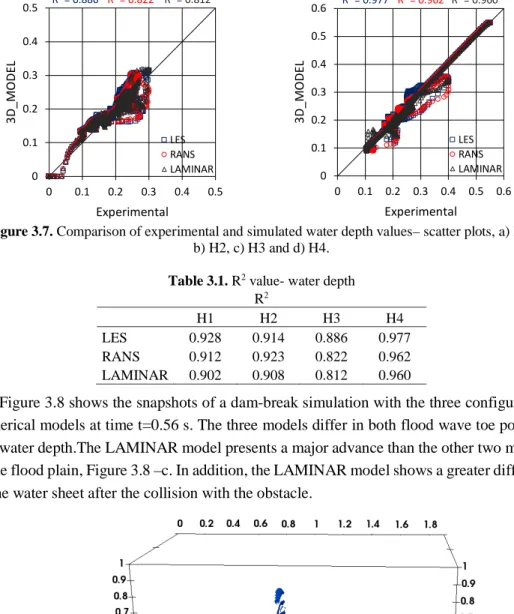
The results demonstrate that the three-dimensional numerical configurations satisfactorily reproduce the temporal variation of the different variables under study with correct trends and high correlation with the experimental values.

Regarding the analysis and prediction of the flow structures, the results show the importance of the turbulence approach in the numerical configuration. On the other hand, the results of the new multi-dimensional two-phase model allow to analyze the full dynamics for sediment transport (concentration profile).

Although the numerical results are satisfactory, the application of three-dimensional numerical models in field-scale cases requires a high computational resource.

Resumen

Este trabajo de investigación se enfoca en el análisis y predicción de las estructuras de flujo y el proceso de transporte de sedimentos en canales abiertos mediante el uso de modelos numéricos tridimensionales.

El estudio numérico se realizó utilizando el software de dinámica de fluidos computacional o CFD (por sus siglas en inglés) basado en el método de volúmenes finitos (FVM) - OpenFOAM. La influencia de la turbulencia es analizada con las dos principales metodologías, LES (Large Eddy Simulation) y RANS (Reynolds-Averaged Navier–Stokes); mientras que el método VOF (Volume of Fluid) es usado para la captura de la superficie libre del agua. Además, se aplica un nuevo modelo multidimensional para el transporte de sedimentos basado en la formulación matemática Euleriana de dos fases.

Los resultados obtenidos de las diferentes configuraciones numéricas son verificados y validados con datos experimentales publicados en importantes revistas de investigación. Las características principales de las diferentes estructuras de flujo se estudian en tres casos que incluyen condiciones de flujo estacionario y no estacionario (también conocido como flujo transitorio). Por otro lado, el nuevo modelo multidimensional para el estudio de transporte de sedimentos se aplica para predecir la socavación producida en un caso experimental de chorro de fondo sobre lecho erosionable.

Los dominios computacionales son configurados con elementos estructurados no uniformes. Además, se realiza un análisis de sensibilidad en cada caso de estudio con el objetivo de obtener resultados independientes del tamaño de mallas utilizadas. Este análisis permite encontrar un equilibrio entre la precisión de los resultados y un tiempo de cálculo óptimo.

Los resultados muestran que las configuraciones numéricas son capaces de reproducir satisfactoriamente las diferentes variables en estudio, con tendencias correctas y una alta correlación con los valores experimentales.

Con respecto al análisis y predicción de las estructuras de flujo, los resultados revelan la importancia que tiene el uso del modelo de turbulencia en la configuración numérica. Por otro lado, los resultados obtenidos con el uso de un nuevo modelo multidimensional de dos fases permiten analizar la dinámica completa del transporte de sedimentos (perfil de concentración).

Aunque los resultados numéricos son satisfactorios, la aplicación de modelos tridimensionales en casos a escala de campo exige un considerable recurso computacional en velocidad de cálculo y almacenamiento de datos.

List of Figures

Figure 2.1. Energy cascade at high Reynolds number – schematic diagram “Adapted from

Pope [6]” ... 7

Figure 2.2. Velocity distribution near the wall “Adapted from Davidson [24]” ... 15

Figure 2.3. General file structure in a simulation case - OpenFOAM ... 17

Figure 2.4. Water-air interface with a volume fraction indicator “Adapted from Rusche [29]” ... 20

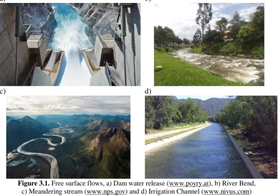
Figure 3.1. Free surface flows, a) Dam water release (www.poyry.at), b) River Bend, c) Meandering stream (www.nps.gov) and d) Irrigation Channel (www.nivus.com) ... 26

Figure 3.2. Schematic view of the experimental set-up “Adapted from Kleefsman et al.[48]” ... 30

Figure 3.3. Schematic view of the Boundary conditions, a) profile view A-A b) profile view B-B (refers Figure 3.2) ... 31

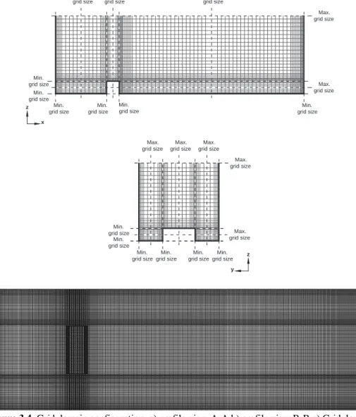
Figure 3.4. Grid domain configuration, a) profile view A-A b) profile view B-B c) Grid domain detail - plan view ... 32

Figure 3.5. Flood wave toe position- a variation on time (profile view A-A) ... 33

Figure 3.6. Measured and simulated water depths – time variation, a) H1, b) H2, c) H3 and d) H4. ... 35

Figure 3.7. Comparison of experimental and simulated water depth values– scatter plots, a) H1, b) H2, c) H3 and d) H4. ... 36

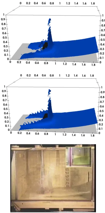
Figure 3.8. Snapshots of a dam-break simulation t=0.56 s. a) LES, b) RANS, c) LAMINAR and d) Experimental photo ( taken from Kleefsman et al. [48]) ... 37

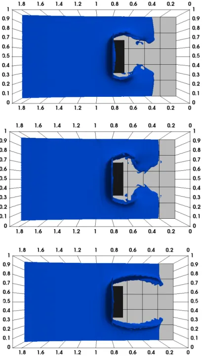
Figure 3.9. A plan view - dam-break simulation t=0.56 s. a) LES, b) RANS, c) LAMINAR ... 38

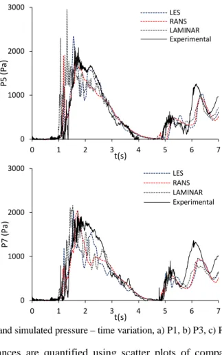
Figure 3.10. Measured and simulated pressure – time variation, a) P1, b) P3, c) P5 and d) P7. ... 40

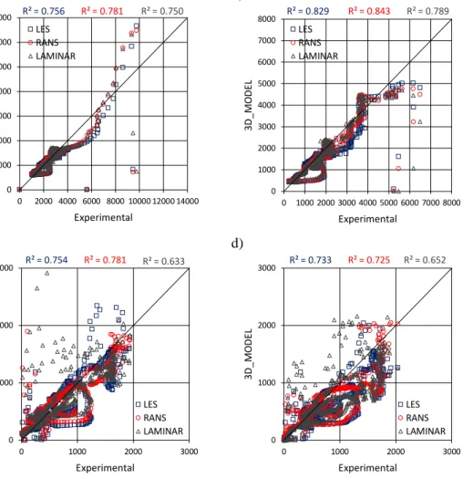
Figure 3.11. Comparison of experimental and simulated pressure values– scatter plots, a) P1, b) P3, c) P5 and d) P7. ... 41

Figure 3.12. Definition variables in an open channel bend – schematic diagram “Adapted from (Blanckaert and De Vried [66])” ... 44

Figure 3.13. A sketch of experimental set-up... 44

Figure 3.14. Cross-sections positions ... 45

Figure 3.15. Description of the boundary conditions- A schematic view... 46

Figure 3.16. a) Grid domain configuration detail - plan view b) Grid domain configuration - plan view c) Bend configuration - detail ... 47

Figure 3.17. Grid domain configuration - cross section ... 48

Figure 3.19. Water surface – snapshots a) RANS, b) LES static, and c) LES dynamic ... 52

Figure 3.20. Measured and simulated profiles- longitudinal velocity component a) section b,b) section d and c) section f. ... 53

Figure 3.21. Streamlines at the established sections, a) section c b) section f. k-ε (RNG)1_{, LES_static}2 _{and LES_dynamic}3_{. ... 54}

Figure 3.22. a) Schematic layout of UPC laboratory channel “adapted from Gómez and Martínez-Gomariz [82]”, b) Schematic view of the channel bend - points for measurements, c) Detail of Section A-A ... 58

Figure 3.23. UPC laboratory channel photos: a) Level sensor, b) sluice gate (taken by Gómez and Martínez- Gomariz [82]) ... 59

Figure 3.24. Schematic view of boundary conditions ... 59

Figure 3.25. Grid domain configuration, a) plan view - detail b) cross-section profile and c) Grid configuration - plan view ... 61

Figure 3.26. Mesh sensitivity analysis- Relative Error estimation - water depth, a) point 3 and b) point 10 ... 62

Figure 3.27. Effective roughness height analysis, a) Point 3, b) Point 10 ... 62

Figure 3.28. Water depth values - comparison ... 63

Figure 3.29.Cross section locations ... 64

Figure 3.30. Open channel bend a) Numerical results b) PAC-UPC laboratory photo (taken by Gómez and Martínez-Gomariz [82]) and c) Free-surface numerical results ... 65

Figure 3.31. Sketch of secondary flows a) first sharp bend –section 60º, b) second sharp bend –section 90º... 65

Figure 3.32. Streamlines at the established sections - first sharp bend a) 0º, b) 30º, c) 45º, d) 60º, and e) 90º ... 67

Figure 3.33. Streamlines at the established sections - second sharp bend a) 0º, b) 45º, and c) 90º ... 68

Figure 3.34. Streamlines at different distances from the bed, a) Near the bed, b) Mid-depth of flow and c) Water surface ... 69

Figure 3.35. Streamlines in a section parallel to the wall - gate and the two outlets influence, a) water phase and the air phase b) water phase ... 69

Figure 3.36. Contours of longitudinal component velocity (m/s) - first sharp bend, a) 0º, b) 30º, c) 45º, d) 60º, and e) 90º... 71

Figure 3.37. Contours of longitudinal component velocity (m/s) -second sharp bend a) 0º, b) 45º, and c) 90º ... 72

Figure 4.1. Scour hole around bridge piers: a) cylindrical (www.usgs.gov) and b) rectangular cylinder (www.fondriest.com); c) Bridge failure due to pier scour (www.iahrmedialibrary.net) ... 80 Figure 4.2. Schematic plot of different mechanisms in sediment transport “Adapted from

Figure 4.3. Slope effect on sediment transport - a single moving particle. “Adapted from Roulund [26]” ... 84 Figure 4.4. Schematic view of the turbulent wall jet scour experiment ... 93 Figure 4.5. Description of the boundary conditions- An schematic view... 94 Figure 4.6. a) A sketch of the numerical domain configuration, b) Grid configuration detail inlet-apron, c) Grid configuration detail apron-sediment ... 96 Figure 4.7. Scour profile development at time: a) 1 min, b) 3 min, c) 5 min and d) 8min. . 99 Figure 4.8. Sediment concentration profiles – scour process: a) 1 min, b) 3 min, c) 5 min and d) 8min (volume fraction indicator field). ... 101 Figure 4.9. Maximum Scour depth - evolution with time ... 102 Figure 4.10. Sediment deposition dune peak - evolution with time, a) height and b) horizontal location ... 102 Figure 4.11. Apron zone before the jet reached the erodible part: a) velocity (m/s), b) water-surface profile (volume fraction indicator field) ... 103 Figure 4.12. Sediment velocity profiles at time a) 1 min, b) 3 min, c) 5 min and d) 8min. ... 105

List of Tables

Table 3.1. R2 _{value- water depth ... 36} Table 3.2. R2 _{value -pressure ... 40} Table 3.3. Boundary conditions implemented in the test-case numerical simulation ... 46 Table 3.4. Water-depth statistic values ... 52 Table 3.5. Hydraulic and geometric characteristics – experimental set-up ... 58 Table 4.1. Constant coefficient values... 89 Table 4.2. Physical parameters for the numerical simulation ... 94 Table 4.3. Boundary conditions implemented in the test-case numerical simulation ... 95 Table 4.4. Summary of the grid size implemented – vertical direction ... 97 Table 4.5. Coefficient of determination R2 _{... 100} Table 4.6. Max. Discrepancy ... 102

List of symbols

Latin alphabet. Lower case

𝑎𝑎𝑖𝑖𝑖𝑖 deviatoric (anisotropic) part - turbulent kinetic energy

𝑐𝑐 sediment mass concentration

𝑐𝑐𝑏𝑏 sediment concentration at the nearest cell center above the bed

𝑐𝑐𝑏𝑏∗ equilibrium sediment concentration at a reference level near the bed

𝑑𝑑 characteristic grand size of the bed material (i.e. 𝑑𝑑₅₀)

𝑑𝑑⊥ normal distance to the wall

𝑒𝑒 coefficient of restitution during collision

𝑓𝑓𝜎𝜎 surface tension

g gravitational acceleration

𝑔𝑔𝑠𝑠0 radial distribution function

𝑘𝑘 turbulent kinetic energy

𝑘𝑘𝑠𝑠 effective roughness height

𝑘𝑘𝑠𝑠𝑠𝑠 _{conductivity of granular temperature}

𝑘𝑘𝑓𝑓 _{modified turbulence kinetic energy (Multiphase Eulerian}

two-phase modeling of sediment transport)

𝑙𝑙𝑜𝑜 integral length scale

𝑙𝑙∗ _{turbulent length scale}

𝑛𝑛 bed porosity

𝐧𝐧 normal unit

𝑝𝑝 pressure, filtered or Reynolds-averaged

𝑝𝑝̅ Reynolds-averaged pressure

𝑝𝑝̂ filtered pressure

𝑝𝑝𝑠𝑠 _{particle pressure}

𝑝𝑝𝑠𝑠𝑠𝑠 _{particle pressure collisional component}

𝑝𝑝𝑠𝑠𝑓𝑓 _{particle pressure frictional component}

𝑞𝑞 contribution from the source of the quantity 𝜙𝜙

𝑞𝑞𝑏𝑏𝑖𝑖 bed load transport rates in different directions (fluxes)

𝑞𝑞𝑖𝑖 flux of granular temperature

𝑟𝑟_{𝑖𝑖𝑖𝑖}𝑓𝑓𝑓𝑓 grain-scale components (Multiphase Eulerian two-phase modeling of sediment transport)

𝑠𝑠 specific density of the sediment

𝑡𝑡 time

𝑡𝑡𝑙𝑙 characteristic timescale of energetic eddies

𝑡𝑡𝑝𝑝 particle response time

𝑢𝑢𝑖𝑖,𝑖𝑖 fluid velocity components

𝑢𝑢�𝑖𝑖,𝑖𝑖 Reynolds-averaged velocities

𝑢𝑢�𝑖𝑖,𝑖𝑖 filtered velocities

𝑢𝑢_𝑖𝑖𝑎𝑎,𝑤𝑤,𝑠𝑠 velocity for air (𝑎𝑎), water (𝑤𝑤) and sediment (𝑠𝑠)

𝑢𝑢∗ _{turbulent velocity scale}

𝑢𝑢∗ shear velocity

𝑢𝑢+ _{dimensionless velocity}

𝑢𝑢𝜂𝜂 Kolmogorov velocity scales

𝐮𝐮 filtered or Reynolds-averaged velocity vector

𝐮𝐮𝐫𝐫 compression velocity

𝑤𝑤𝑠𝑠 sediment fall velocity

𝑥𝑥𝑖𝑖,𝑖𝑖 Cartesian coordinates

𝑦𝑦+ _{normalized distance to the wall}

𝑧𝑧𝑏𝑏 reference level near the bed

Latin alphabet. Upper case

𝐵𝐵 empirical coefficient (Multiphase Eulerian two-phase modeling of

sediment transport)

𝐶𝐶 constant that reflects the slope of the sediment flux 𝐶𝐶𝑚𝑚𝑎𝑎𝑚𝑚 maximum Courant number

𝐶𝐶𝑜𝑜 courant number

𝐶𝐶𝑠𝑠 constant Smagorinsky coefficient

𝐶𝐶𝛼𝛼 controls the intensity of the compression

𝐶𝐶𝜀𝜀1 constant Standard 𝑘𝑘 − 𝜀𝜀 model

𝐶𝐶𝜀𝜀2 constant Standard 𝑘𝑘 − 𝜀𝜀 model

𝐶𝐶𝜀𝜀13 constant Renormalization Group (RNG) k-ε turbulence model

𝐶𝐶𝜔𝜔12 constant 𝑘𝑘 − 𝜔𝜔 model

𝐶𝐶𝜔𝜔22 constant 𝑘𝑘 − 𝜔𝜔 model

𝐶𝐶𝜇𝜇 constant Standard 𝑘𝑘 − 𝜀𝜀 model

𝐶𝐶𝜇𝜇RNG constant Renormalization Group (RNG) k-ε turbulence model

𝐶𝐶1𝜀𝜀, 𝐶𝐶2𝜀𝜀, 𝐶𝐶3𝜀𝜀, 𝐶𝐶4𝜀𝜀,

𝐶𝐶𝜇𝜇

constants Multiphase Eulerian two-phase modeling of sediment transport

𝐷𝐷 flow field domain (LES model)/ deposition rate (Single-phase sediment transport model)

𝐷𝐷∗ dimensionless particle diameter

𝐸𝐸 entrainment /erosion rate

𝐺𝐺 function filter

𝐻𝐻 water depth from bed

𝐽𝐽𝑖𝑖𝑖𝑖𝑓𝑓 energy production / dissipation - interaction with the carrier fluid

𝐿𝐿 characteristic length of the involve geometries

ℒ𝑖𝑖𝑖𝑖 Germano identity

𝑀𝑀_𝑖𝑖𝑓𝑓𝑠𝑠, 𝑀𝑀_𝑖𝑖𝑠𝑠𝑓𝑓 interphase momentum (Multiphase Eulerian two-phase modeling of sediment transport)

N number of identical experiments at a certain time - Reynolds

averaging analysis

𝑃𝑃𝑘𝑘 turbulent production

𝑅𝑅 relative submerged density

𝑅𝑅𝑒𝑒 Reynolds number

𝑅𝑅2 _{Coefficient of determination}

𝑅𝑅_{𝑖𝑖𝑖𝑖}𝑓𝑓𝑓𝑓 Reynolds stress (Multiphase Eulerian two-phase modeling of sediment transport)

𝐑𝐑 Reynolds stress (RANS) or subgrid-scale Reynolds stress (LES)

𝑆𝑆 surface in a control volume

𝑆𝑆̂𝑖𝑖𝑖𝑖 strain rate of the large scale or resolved field strain rate tensor

𝑆𝑆_{𝑖𝑖𝑖𝑖}𝑓𝑓 fluid-phase strain rate tensor (Multiphase Eulerian two-phase modeling of sediment transport)

𝑆𝑆𝑖𝑖𝑖𝑖 strain-rate tensor

𝑆𝑆𝑓𝑓 Stokes number

𝐒𝐒 strain rate – tensor notation

𝑇𝑇 Time interval over which averaging is performed - Reynolds

averaging analysis

𝑈𝑈 characteristic velocity of the flow

𝐔𝐔 magnitude absolute velocity

𝑉𝑉 volume in a control volume

𝑉𝑉𝑓𝑓 volumes occupied by the interstitial fluid

𝑉𝑉𝑃𝑃 volumes occupied by the particles

Greek alphabet. Lower case

𝛼𝛼 volume fraction (VOF method)/ Turbulence drag parameter

(Multiphase Eulerian two-phase modeling of sediment transport)

𝛽𝛽 constant Renormalization Group (RNG) k-ε turbulence model/ bed

slope angle (Single-phase sediment transport model)

𝛾𝛾𝑠𝑠 energy dissipation rate

𝛿𝛿𝑖𝑖𝑖𝑖 Kronecker delta

𝛿𝛿𝜈𝜈 viscous length scale

𝜀𝜀 turbulent kinetic energy dissipation rate

𝜂𝜂 Kolmogorov length scales/ bed elevation (Single-phase sediment

transport model)

𝜃𝜃 dimensionless bed shear stress (Shield number) / granular

temperature (Multiphase Eulerian two-phase modeling of sediment transport)

𝜃𝜃𝑠𝑠 critical Shields number for initiation of motion

𝜃𝜃𝑠𝑠𝑜𝑜 critical Shield number for initiation of motion at the horizontal bed

𝜃𝜃𝑓𝑓 constant friction angle (repose angle)

𝜅𝜅 Von Karman´s constant

𝜅𝜅𝛼𝛼 curvature of the interface

𝜆𝜆 bulk viscosity

𝜇𝜇 viscosity

𝜇𝜇𝑠𝑠 static friction coefficient

𝜇𝜇𝑠𝑠𝑠𝑠𝑠𝑠 subgrid eddy viscosity

𝜇𝜇𝑓𝑓 eddy viscosity

𝜇𝜇𝑠𝑠𝑠𝑠 _{particle shear viscosity}

𝜌𝜌 fluid density

𝜌𝜌𝑤𝑤 density of water

𝜌𝜌𝑓𝑓 volume force term

𝜎𝜎 surface tension coefficient

𝜎𝜎𝑠𝑠 turbulent Schmidt number

𝜎𝜎𝑘𝑘 constant Standard 𝑘𝑘 − 𝜀𝜀 model

𝜎𝜎𝑘𝑘1 constant 𝑘𝑘 − 𝜔𝜔 model

𝜎𝜎𝑘𝑘2 constant Renormalization Group (RNG) k-ε turbulence model

𝜎𝜎𝜀𝜀 constant Standard 𝑘𝑘 − 𝜀𝜀 model

𝜎𝜎𝜀𝜀2 constant Renormalization Group (RNG) k-ε turbulence model

𝜎𝜎𝜔𝜔1 constant 𝑘𝑘 − 𝜔𝜔 model

𝜈𝜈𝑓𝑓 diffusivity

𝜙𝜙 scalar or vector quantity

𝜙𝜙𝑎𝑎,𝑤𝑤,𝑠𝑠 _{volumetric concentration for air (𝑎𝑎), water (𝑤𝑤) and sediment (𝑠𝑠)}

𝜙𝜙𝑓𝑓 _{fluid phase}

𝜙𝜙(𝑥𝑥,𝑡𝑡) flow variables - Reynolds averaging analysis

𝜙𝜙�(𝑥𝑥,𝑡𝑡) mean value component - Reynolds averaging analysis 𝜙𝜙′_{(𝑥𝑥,𝑡𝑡) fluctuating component - Reynolds averaging analysis}

𝜙𝜙�(𝑥𝑥,𝑡𝑡)

��������� time average over a time-averaged quantity

𝜙𝜙′(𝑥𝑥,𝑡𝑡)

���������� time average over a fluctuating quantity

𝜙𝜙_𝑓𝑓𝑠𝑠 _{random-loose-packing concentration for spheres}

𝜙𝜙𝑚𝑚𝑎𝑎𝑚𝑚𝑠𝑠 random-close-packing concentration for spheres

𝜑𝜑 angle between the fluid velocity vector at the particle position and the steepest bed slope direction

𝜂𝜂0 constant Renormalization Group (RNG) k-ε turbulence model

𝜏𝜏𝑏𝑏 boundary shear stress/bed shear stress (Single-phase sediment

transport model)

𝜏𝜏𝑖𝑖𝑖𝑖 Reynolds stresses

𝜏𝜏𝜂𝜂 Kolmogorov time scales

𝜏𝜏𝑖𝑖𝑖𝑖𝑠𝑠𝑠𝑠 particle stress collisional component

𝜏𝜏𝑖𝑖𝑖𝑖𝑠𝑠𝑓𝑓 particle stress frictional component

𝜏𝜏_{𝑖𝑖𝑖𝑖}𝑓𝑓 fluid stress (Multiphase Eulerian two-phase modeling of sediment transport)

𝜏𝜏_{𝑖𝑖𝑖𝑖}𝑠𝑠 _{particle shear stress}

𝜐𝜐 dynamic viscosity

𝜐𝜐𝑓𝑓𝑓𝑓 _{turbulent eddy viscosity}

𝜓𝜓 dimensionless shear stress parameter

Greek alphabet. Upper case

Γ diffusion coefficient

Δ filter cutoff width –LES

∆𝑙𝑙 characteristic length of grid size

Δ� additional test filter

Τ𝑖𝑖𝑖𝑖𝑠𝑠𝑠𝑠𝑠𝑠 test filtering

Φ variables- LES model

Φ� filtered (resolved) variable- LES

1

INTRODUCTION

1.1 Background and motivation

The prediction of flow and sediment transport in open-channels and rivers presents a significant challenge for river engineering. Flows in natural and artificial channel systems commonly encounter the interaction between a variety of planimetries (i.e. curved and braided channels) and/or structures (i.e. bridge piers, weirs, dams, barrages, intakes, etc.) which usually produce a three-dimensional effect, free-surface variation and bed change that significantly affect the flow structure and the sediment transport process.

Early numerical models based on a set of algebraic and differential equations in one- and two- dimensional approaches have been developed. These numerical models are applied where the vertical velocities and accelerations are negligible, resulting in a hydrostatic pressure distribution.

Recently, the development in computer capabilities has provided the use of three-dimensional numerical models which are based on the application of the Navier-Stokes equations. This numerical approach allows a better representation of the complex process involved, providing a new insight and understanding concerning in river engineering analysis.

Computational Fluid Dynamics (CFD), its fundamental basis being the Navier–Stokes equations, allows the solving of river engineering problems using numerical methods. CFD codes are tools that permit to evaluate different combinations of boundary conditions, geometric changes and also reduce scale-up problems presented in the experimental models. This implies the analysis of the advantages and disadvantages obtained whenever three-dimensional numerical models are applied in river engineering issues. There is a significant value in identifying the flow structure and sediment transport process in which this numeric approach becomes more important.

1.2 Objectives 1.2.1 Main objective

The main goal of this study is TO USE THREE-DIMENSIONAL NUMERICAL MODELS TO ANALYZE AND PREDICT THE FLOW STRUCTURE AND SEDIMENT

TRANSPORT PROCESS IN OPEN-CHANNELS. Also, it is expected that the conclusions reached would provide an insight into the applications for which the hydrostatic pressure distribution assumption is no longer valid.

1.2.2 Specific Objectives

In order to reach the aforementioned main goals, the following specific targets are pursued:

 Review of the mathematical governing equations that represent the variables involved in both the flow structure and the sediment transport process.

 Understand the importance of the turbulence model and free-surface variation in order to identify the most important flow dynamics processes.

 Select some representative experimental set-up cases for which the three-dimensional effect is important.

 Perform mesh sensitive analysis to obtain results no matter the grid configuration size.

 Verify the accuracy and reliability of the three-dimensional numerical configuration models against experimental results.

 Issue general conclusions regarding the relevance of using a new multi-dimensional numerical approach in the analysis of the sediment transport process.

 Show the key processes and the main results concerning the river channel dynamics.

1.3 Methodology

The three-dimensional study in this research project is developed on the open-source computational fluid dynamics (CFD) code named OpenFOAM. The source code accessibility facilitates the addition/customization of features required in river engineering problems.

The following items describe in detail the steps carried out in this investigation to achieve each of the above specific objectives.

 Review of governing equations. The derivation of the governing equations provides the basic knowledge of the fundamentals involved in the three-dimensional numerical simulation. As well, it allows to understand the importance of the use of the turbulence models, the method to track/capture the free surface and the significance of the boundary conditions.

 Validating the numerical results with experimental data. Different numerical configurations in steady and unsteady-state (transient) hydraulic flow conditions are analyzed in order to identify the main characteristics of the fluid dynamics processes.

 Numerical models of sediment transport. A new multi-dimensional numerical model to analyze the sediment transport process is applied to predict the local scour

Chapter 1 Introduction

caused by a submerged wall jet. To the author’s knowledge, this test-case numerical analysis using the kinetic theory has not been reported in the literature.

1.4 Outline of the thesis

Subsequently, the thesis is organized as follows:

The next section, Chapter 2, provides the theoretical background needed for the comprehensive use of a three-dimensional numerical model. The third chapter contains the three-dimensional numerical simulation of three cases in steady and unsteady-state flow conditions to identify the flow dynamics processes involved. Chapter 4 describes the mathematical formulation considered to simulate the sediment transport process. An application to a scouring process is presented. Finally, Chapter 5 presents a summary of the overall conclusions of this research project.

2

GOVERNING EQUATIONS

2.1 Introduction

This chapter provides an overview of the basic mathematical equations required to describe the three-dimensional free-surface flow simulations in river engineering applications. The Navier-Stokes equations for an incompressible viscous flow that represent the physics conservation law properties and the models used to simplify the resolution of turbulent flows based on LES and RANS approaches are described.

The numerical model based on the Finite Volume Method (FVM), the free-surface model founded on the Volume of Fluid method (VOF) and the most common boundary conditions are discussed.

2.2 The Navier-Stokes equations

The governing equations for the fluid flow in hydraulic engineering applications are the incompressible Navier-Stokes equations for Newtonian fluids. These equations consist of the law of conservation of mass ( 2.1 ) and the law of conservation of momentum ( 2.2), which are presented in Eulerian form. The mass conservation equation is also called the continuity equation, which states that since the matter is neither created nor destroyed, it can only be transformed by physical, chemical or biological processes; whereas, the momentum conservation or equation of motion is a vector quantity defined as a product of mass and velocity. 𝜕𝜕𝑢𝑢𝑖𝑖 𝜕𝜕𝑥𝑥𝑖𝑖 = 0 ( 2.1 ) 𝜕𝜕𝑢𝑢𝑖𝑖 𝜕𝜕𝑡𝑡 +𝑢𝑢𝑖𝑖𝜕𝜕𝑢𝑢_{𝜕𝜕𝑥𝑥}𝑖𝑖 𝑖𝑖 =− 1 𝜌𝜌 𝜕𝜕𝑝𝑝 𝜕𝜕𝑥𝑥𝑖𝑖+𝜐𝜐 𝜕𝜕2_𝑢𝑢 𝑖𝑖 𝜕𝜕𝑥𝑥𝑖𝑖𝜕𝜕𝑥𝑥𝑖𝑖 ( 2.2 )

where 𝑖𝑖,𝑗𝑗= 1,2,3 is the tensor notation (Cartesian coordinates), 𝑢𝑢_𝑖𝑖 are the fluid velocity components, 𝑝𝑝 is the pressure, 𝜌𝜌 is the fluid density and 𝜐𝜐 is the dynamic viscosity, defined as the viscosity 𝜇𝜇 divided by 𝜌𝜌. The pressure presents a particular situation, in which it does not appear under a time dependence form, and it is only determined up to a constant. This requires special treatment for numerical schemes in order to solve continuity [1,2].

𝑅𝑅𝑒𝑒=𝜌𝜌𝑈𝑈𝐿𝐿_𝜇𝜇 ( 2.3 ) here, 𝑈𝑈is the characteristic velocity of the flow and 𝐿𝐿 is a characteristic length of the involve geometries.

Laminar flows, at low Reynolds numbers, are stable due to viscous term are dominant and hence the momentum equation becomes more linear. On the other hand, turbulent flows, at high Reynolds numbers, are unsteady, chaotic, random, and involve three-dimensional fluctuations where, inertial term dominates, causing non-linearity in the momentum equation.

2.3 Turbulent scales

The modern theory of turbulence is based on the energy cascade concept first introduced by Richardson [3] and quantified by Kolmogorov [4]. In this theory, turbulence is composed of different scales of flow motion referred as eddies. Through the cascade process, Figure 2.1, the kinetic energy is transferred from largest scales (production mechanism resulting from the flow shear) to smaller and smaller scales by inviscid process (inertia effect) until, at the smallest scales, the friction forces (viscous stresses) become large and the kinetic energy is dissipated as heat. The kinetic energy rate transferred from an eddy to a smaller eddy is the same for each eddy size [5], resulting in equal to the turbulent kinetic energy dissipation rate, 𝜀𝜀.

Through dimensional analysis, the smallest scales of turbulent motion, where dissipation occurs, can be defined based on a set of two parameters, 𝜀𝜀 [𝐿𝐿2⁄𝑇𝑇3] and 𝜐𝜐 [𝐿𝐿2⁄𝑇𝑇], i.e. Kolmogorov length (𝜂𝜂), time �𝜏𝜏_𝜂𝜂� and velocity �𝑢𝑢_𝜂𝜂� scales.

𝜂𝜂=�𝜐𝜐_{𝜀𝜀 �}3

1 4⁄

𝜏𝜏𝜂𝜂=�𝜐𝜐_𝜀𝜀�

1 2⁄

𝑢𝑢𝜂𝜂= (𝜀𝜀𝜐𝜐)1 4⁄ ( 2.4 )

The Reynolds number of the Kolmogorov scales is one, i.e. 𝜂𝜂𝑢𝑢_𝜂𝜂⁄𝜐𝜐= 1 , which is small enough for the dissipation of the kinetic energy to be effective (see Pope [6]). Additionally, the largest scales of turbulent motion (𝑙𝑙_𝑜𝑜- integral length scale) are determined by the characteristic size of the flow.

Chapter 2 Governing Equations

Figure 2.1. Energy cascade at high Reynolds number – schematic diagram “Adapted from Pope [6]”

Navier Stokes equations describe both laminar and turbulent flow, but the spatial resolution required to solve the whole range of the turbulent scales for practical hydraulic engineering problems makes Direct Numerical Simulation (DNS) approach out of reach based on the current computer capacities (the total computational effort for DNS simulations is proportional to Re3 _{for homogeneous turbulence [1]).}

In order to reduce computational cost, statistical analysis can be used to avoid the solution of all the scales of flow motion. There are basically two main methodologies. The first one, called Large Eddy Simulation (LES), which directly solves the largest scales of flow motion while modeling only the small scales. On the other hand, the second approach, called the Reynolds-Averaged Navier–Stokes (RANS), parameterizes all turbulent fluctuations presenting the calculation of the turbulent averaged flow.

2.4 Reynolds-Averaged Navier–Stokes (RANS) 2.4.1 Reynolds Averaging

The Reynolds averaging concept introduced by Reynolds [7], is used to derive the equations of motion for time-averaged turbulent quantities. The main idea behind of Reynolds averaging is to decompose any of the flow variables involved,𝜙𝜙(𝑥𝑥,𝑡𝑡), which is a function of time and space, into a mean value component,𝜙𝜙�(𝑥𝑥,𝑡𝑡), and a fluctuating component, 𝜙𝜙′_{(𝑥𝑥,𝑡𝑡), which is of a stochastic nature.}

𝜙𝜙(𝑥𝑥,𝑡𝑡) =𝜙𝜙�(𝑥𝑥,𝑡𝑡) +𝜙𝜙′(𝑥𝑥,𝑡𝑡) ( 2.5 ) The mean value, 𝜙𝜙�(𝑥𝑥,𝑡𝑡), can be computed by using any of the following perceptions: time averaging (average of a quantity over a time interval), space averaging (average of a quantity over a space interval) or ensemble averaging (average of numerous identical quantities at a certain time) [8].

The time averaging approach is appropriate when considering a steady turbulent flow (flow does not vary on the average in time)

L

lo lEI

Dissipation range

Inertial sub-range Energy containing

range Dissipation energy to

succesively smaller scales

Dissipation Production P

T(l)

𝜙𝜙�(𝑥𝑥) = lim_{𝑇𝑇→∞}1_{𝑇𝑇 � 𝜙𝜙}𝑓𝑓+𝑇𝑇 (𝑥𝑥,𝑡𝑡) 𝑑𝑑𝑡𝑡

𝑓𝑓

( 2.6 ) here, 𝑇𝑇 is the time interval over which averaging is performed and for engineering applications, it is assumed that, it is much greater compared to the time scale of the turbulent fluctuations.

If unsteady flow occurs, with time scales of the same order of the turbulent fluctuations, the ensemble averaging must be used. Ensemble average should be understood as an average of N identical experiments at a certain time, which is both time and space-dependent.

𝜙𝜙�(𝑥𝑥,𝑡𝑡) = lim_{𝑇𝑇→∞𝑁𝑁 � 𝜙𝜙}1 (𝑥𝑥,𝑡𝑡)

𝑁𝑁

𝑖𝑖=1

( 2.7 )

2.4.2 Averaging Rules

Some of the averaging rules are needed in deriving RANS equations, which include,

 The time average over a time-averaged quantity gives the same time average

𝜙𝜙�(𝑥𝑥,𝑡𝑡)

���������_{=𝜙𝜙�(𝑥𝑥,𝑡𝑡)} ( 2.8 )

 The time average over a fluctuating quantity is zero.

𝜙𝜙′(𝑥𝑥,𝑡𝑡)

����������_{= 0} ( 2.9 )

In the ensemble average as the averaging operation, i.e.

𝜕𝜕𝜙𝜙𝚤𝚤 𝜕𝜕𝑥𝑥𝚤𝚤 ����� =𝜕𝜕𝜙𝜙�_{𝜕𝜕𝑥𝑥}𝑖𝑖 𝑖𝑖 ( 2.10 ) 𝜕𝜕𝜙𝜙𝚤𝚤 𝜕𝜕𝑡𝑡 ����� =𝜕𝜕𝜙𝜙�_{𝜕𝜕𝑡𝑡}𝑖𝑖 ( 2.11 )

2.4.3 Incompressible RANS equations

The RANS equations are derived from applying the rules ( 2.8 )-( 2.11 ) in the Navier-Stokes equations ( 2.1 ) and ( 2.2 ) 𝜕𝜕𝑢𝑢�𝑖𝑖 𝜕𝜕𝑥𝑥𝑖𝑖 = 0 ( 2.12 ) 𝜕𝜕𝜌𝜌𝑢𝑢�𝑖𝑖 𝜕𝜕𝑡𝑡 + 𝜕𝜕𝜌𝜌𝑢𝑢�𝑖𝑖𝑢𝑢�𝑖𝑖 𝜕𝜕𝑥𝑥𝑖𝑖 =− 𝜕𝜕𝑝𝑝̅ 𝜕𝜕𝑥𝑥𝑖𝑖+ 𝜕𝜕 𝜕𝜕𝑥𝑥𝑖𝑖�𝜇𝜇 � 𝜕𝜕𝑢𝑢�𝑖𝑖 𝜕𝜕𝑥𝑥𝑖𝑖 + 𝜕𝜕𝑢𝑢�𝑖𝑖 𝜕𝜕𝑥𝑥𝑖𝑖��+ 𝜕𝜕𝜏𝜏𝑖𝑖𝑖𝑖 𝜕𝜕𝑥𝑥𝑖𝑖 ( 2.13 ) where 𝑢𝑢�_𝑖𝑖 and 𝑢𝑢�_𝑖𝑖 are Reynolds-averaged velocities and 𝑝𝑝̅ is the Reynolds-averaged pressure.

The difference between RANS equations and Navier-Stokes equations is that, an additional term,𝜏𝜏_{𝑖𝑖𝑖𝑖} , called Reynolds stresses, is introduced.

Chapter 2 Governing Equations

Reynolds stress is a symmetric second-order tensor, where the diagonal components are the normal stresses and the off-diagonal components are shear stresses.

𝜏𝜏𝑖𝑖𝑖𝑖 =−𝜌𝜌 � 𝑢𝑢𝚤𝚤′2 ����� _{𝑢𝑢������� 𝑢𝑢𝚤𝚤′𝑢𝑢𝚥𝚥′} ��������_{𝚤𝚤′𝑢𝑢𝑘𝑘′} 𝑢𝑢𝚥𝚥′𝑢𝑢𝚤𝚤′ ������� _𝑢𝑢�����_𝚥𝚥′2 _𝑢𝑢��������_{𝚥𝚥′𝑢𝑢𝑘𝑘′} 𝑢𝑢𝑘𝑘′𝑢𝑢𝚤𝚤′ �������� 𝑢𝑢�������� 𝑢𝑢𝑘𝑘′𝑢𝑢𝚥𝚥′ ������𝑘𝑘′2 �

Note that new unknown terms are introduced; consequently, the system is not closed and an additional model denominated turbulence model is required.

The turbulent kinetic energy is the half of the trace of the Reynolds stress

𝑘𝑘=1₂𝜌𝜌𝑢𝑢′�������𝚤𝚤𝑢𝑢′𝚥𝚥 =1₂𝜌𝜌�𝑢𝑢�����𝚤𝚤′2+𝑢𝑢�����𝚥𝚥′2+𝑢𝑢�������𝑘𝑘′2 ( 2.15 )

Thus, the isotropic stress is defined as 2

3𝑘𝑘𝛿𝛿𝑖𝑖𝑖𝑖 and deviatoric (anisotropic) part is

𝑎𝑎𝑖𝑖𝑖𝑖 =𝜌𝜌𝑢𝑢′������� −𝚤𝚤𝑢𝑢′𝚥𝚥 2₃𝑘𝑘𝛿𝛿𝑖𝑖𝑖𝑖 ( 2.16 )

By substituting Equation ( 2.16 ) into Equation ( 2.13 ), the isotropic term is usually combined with the Reynolds-averaged pressure term,𝑝𝑝̅ ← 𝑝𝑝̅+2

3𝑘𝑘𝛿𝛿𝑖𝑖𝑖𝑖 , and a turbulent

closure model is necessary specifically for the deviatoric part (with a negative sign), −𝑎𝑎_{𝑖𝑖𝑖𝑖} ‡_. 2.4.4 The turbulent-viscosity hypothesis

The turbulent-viscosity hypothesis was introduced by Boussinesq. Reynolds stresses are linked to the velocity gradients via the positive scalar coefficient denominated eddy viscosity,𝜇𝜇_𝑓𝑓; following a relation similar to Newtonian fluids.

𝜏𝜏𝑖𝑖𝑖𝑖 =𝜌𝜌𝑢𝑢�������′𝚤𝚤𝑢𝑢′𝚥𝚥 =𝜇𝜇𝑓𝑓�𝜕𝜕𝑢𝑢�_{𝜕𝜕𝑥𝑥}𝑖𝑖 𝑖𝑖 + 𝜕𝜕𝑢𝑢�𝑖𝑖 𝜕𝜕𝑥𝑥𝑖𝑖� − 2 3𝑘𝑘𝛿𝛿𝑖𝑖𝑖𝑖 ( 2.17 ) from where −𝑎𝑎𝑖𝑖𝑖𝑖=−𝜌𝜌𝑢𝑢�������′𝚤𝚤𝑢𝑢′𝚥𝚥+2₃𝑘𝑘𝛿𝛿𝑖𝑖𝑖𝑖=𝜇𝜇𝑓𝑓�𝜕𝜕𝑢𝑢�_{𝜕𝜕𝑥𝑥}𝑖𝑖 𝑖𝑖+ 𝜕𝜕𝑢𝑢�𝑖𝑖 𝜕𝜕𝑥𝑥𝑖𝑖� ( 2.18 ) 2.4.5 Turbulence Models

There are numerous turbulence models based on the Boussinesq hypothesis in the literature. In these models, the eddy viscosity, 𝜇𝜇_𝑓𝑓, can be expressed as a turbulent velocity scale,𝑢𝑢∗, multiplied with a turbulent length scale,𝑙𝑙∗.

𝜇𝜇𝑓𝑓∝ 𝑢𝑢∗𝑙𝑙∗ ( 2.19 )

The turbulence models range from simple algebraic models to highly sophisticated models and can be grouped into four main categories: Algebraic (Zero-Equations), One-Equations, Two- Equations and Second-Order Closure models [8]. Despite the variety of models developed, none is applicable to all flow conditions.

2.4.6 Two-equation turbulence models

In this study, two-equation turbulence models are used because are the most popular models to simulate a large number of engineering flows [9]. These models require the solution of two transport equation, for both the turbulent kinetic energy and the turbulence length scale. Thus, two-equation models are considered complete because no additional information about turbulence is required. The turbulent kinetic energy is generally chosen as one of the transport equations due to its extensive use and easy interpretation.

The transport equation of turbulent kinetic energy (TKE), 𝑘𝑘, describes how mean flow feeds kinetic energy into turbulence. 𝑘𝑘 energy is derived analytically from the Navier-Stokes equations using the Reynolds average kinetic energy of a turbulent flow concept. Further, with some mathematical manipulation, the 𝑘𝑘 equation is obtained. The full derivation of the equation is given in Celik [9]. Three different turbulence closures are employed in this study.

Standard 𝒌𝒌 − 𝜺𝜺 model

In the 𝑘𝑘 − 𝜀𝜀 model of Launder and Spalding [10], the eddy viscosity is modeled as

𝜇𝜇𝑓𝑓=𝜌𝜌𝐶𝐶𝜇𝜇𝑘𝑘

2

𝜀𝜀 ( 2.20 )

The 𝑘𝑘 equation is computed by

𝜕𝜕(𝜌𝜌𝑘𝑘) 𝜕𝜕𝑡𝑡 + 𝜕𝜕(𝜌𝜌𝑢𝑢� 𝑘𝑘𝚤𝚤 ) 𝜕𝜕𝑥𝑥𝑖𝑖 = 𝜕𝜕 𝜕𝜕𝑥𝑥𝑖𝑖��𝜇𝜇+ 𝜇𝜇𝑓𝑓 𝜎𝜎𝑘𝑘� 𝜕𝜕𝑘𝑘 𝜕𝜕𝑥𝑥𝑖𝑖�+𝑃𝑃𝑘𝑘− 𝜌𝜌𝜀𝜀 ( 2.21 )

here 𝑃𝑃_𝑘𝑘 is the turbulent production due to the gradient of the mean flow velocity

𝑃𝑃𝑘𝑘=−𝜌𝜌𝑢𝑢�������′𝚤𝚤𝑢𝑢′𝚥𝚥 𝜕𝜕𝑢𝑢�_{𝜕𝜕𝑥𝑥}𝑖𝑖

𝑖𝑖 ( 2.22 )

𝜎𝜎𝑘𝑘 is an empirical coefficient controlling the magnitude of the diffusion of 𝑘𝑘.

The turbulent dissipation rate,𝜀𝜀 , is modeled based on the energy transfer rate in the energy cascade concept and it is determined by the large-scale motion [6]. The 𝜀𝜀 transport equation is derived in a similar way to 𝑘𝑘.

𝜕𝜕(𝜌𝜌𝜀𝜀) 𝜕𝜕𝑡𝑡 + 𝜕𝜕(𝜌𝜌𝑢𝑢� 𝜀𝜀𝚤𝚤 ) 𝜕𝜕𝑥𝑥𝑖𝑖 = 𝜕𝜕 𝜕𝜕𝑥𝑥𝑖𝑖��𝜇𝜇+ 𝜇𝜇𝑓𝑓 𝜎𝜎𝜀𝜀� 𝜕𝜕𝜀𝜀 𝜕𝜕𝑥𝑥𝑖𝑖�+𝐶𝐶𝜀𝜀1 𝜀𝜀 𝑘𝑘 𝑃𝑃𝑘𝑘− 𝐶𝐶𝜀𝜀2𝜌𝜌 𝜀𝜀2 𝑘𝑘 ( 2.23 )

Chapter 2 Governing Equations

The second and third terms on the right-hand side of Equation ( 2.23 ) are referred to the production and the destruction of 𝜀𝜀, respectively.

The model constants are obtained from simple flow experiments. 𝐶𝐶𝜇𝜇= 0.09, 𝜎𝜎𝑘𝑘= 1,𝜎𝜎𝜀𝜀= 1.3, 𝐶𝐶𝜀𝜀1= 1.44 and 𝐶𝐶𝜀𝜀2= 1.92.

𝒌𝒌 − 𝝎𝝎 model

The k-ω model of Wilcox [11] differs from 𝑘𝑘 − 𝜀𝜀 model, in the fact that 𝜀𝜀 is not modeled. A transport equation is implemented for the specific turbulent dissipation rate,𝜔𝜔.

The eddy viscosity is

𝜇𝜇𝑓𝑓=𝜌𝜌_𝜔𝜔𝑘𝑘 ( 2.24 ) with 𝜔𝜔=

𝜀𝜀

𝐶𝐶𝜇𝜇𝑘𝑘 ( 2.25 )

The 𝑘𝑘 and 𝜔𝜔 transport equations are depicted in the Equations ( 2.26 ) and ( 2.27 )

𝜕𝜕(𝜌𝜌𝑘𝑘) 𝜕𝜕𝑡𝑡 + 𝜕𝜕(𝜌𝜌𝑢𝑢� 𝑘𝑘𝚤𝚤 ) 𝜕𝜕𝑥𝑥𝑖𝑖 = 𝜕𝜕 𝜕𝜕𝑥𝑥𝑖𝑖��𝜇𝜇+ 𝜇𝜇𝑓𝑓 𝜎𝜎𝑘𝑘1� 𝜕𝜕𝑘𝑘 𝜕𝜕𝑥𝑥𝑖𝑖�+𝑃𝑃𝑘𝑘− 𝐶𝐶𝜇𝜇𝜌𝜌𝑘𝑘𝜔𝜔 ( 2.26 ) 𝜕𝜕(𝜌𝜌𝜔𝜔) 𝜕𝜕𝑡𝑡 + 𝜕𝜕(𝜌𝜌𝑢𝑢� 𝜔𝜔𝚤𝚤 ) 𝜕𝜕𝑥𝑥𝑖𝑖 = 𝜕𝜕 𝜕𝜕𝑥𝑥𝑖𝑖��𝜇𝜇+ 𝜇𝜇𝑓𝑓 𝜎𝜎𝜔𝜔1� 𝜕𝜕𝜔𝜔 𝜕𝜕𝑥𝑥𝑖𝑖�+𝐶𝐶𝜔𝜔12 𝜔𝜔 𝑘𝑘 𝑃𝑃𝑘𝑘− 𝐶𝐶𝜔𝜔22𝜌𝜌𝜔𝜔2 ( 2.27 )

with the model constants 𝜎𝜎_𝑘𝑘1 = 2 , 𝜎𝜎_𝜔𝜔1= 2 while the coefficients 𝐶𝐶_𝜇𝜇, 𝐶𝐶_𝜔𝜔12 and 𝐶𝐶_𝜔𝜔22 employ standard values 0.09, 0.55 and 0.075, respectively.

Renormalization Group (RNG) k-ε turbulence model

In the 𝑘𝑘 − 𝜀𝜀 (RNG) model introduced by Yakhot and Orszag [12], the eddy viscosity is computed as

𝜇𝜇𝑓𝑓=𝜌𝜌𝐶𝐶𝜇𝜇RNG𝑘𝑘 2

𝜀𝜀 ( 2.28 )

The turbulent kinetic energy and dissipation rate, respectively are

𝜕𝜕(𝜌𝜌𝑘𝑘) 𝜕𝜕𝑡𝑡 + 𝜕𝜕(𝜌𝜌𝑢𝑢� 𝑘𝑘𝚤𝚤 ) 𝜕𝜕𝑥𝑥𝑖𝑖 = 𝜕𝜕 𝜕𝜕𝑥𝑥𝑖𝑖��𝜇𝜇+ 𝜇𝜇𝑓𝑓 𝜎𝜎𝑘𝑘� 𝜕𝜕𝑘𝑘 𝜕𝜕𝑥𝑥𝑖𝑖�+𝑃𝑃𝑘𝑘− 𝜌𝜌𝜀𝜀 ( 2.29 ) 𝜕𝜕(𝜌𝜌𝜀𝜀) 𝜕𝜕𝑡𝑡 + 𝜕𝜕(𝜌𝜌𝑢𝑢� 𝜀𝜀𝚤𝚤 ) 𝜕𝜕𝑥𝑥𝑖𝑖 = 𝜕𝜕 𝜕𝜕𝑥𝑥𝑖𝑖��𝜇𝜇+ 𝜇𝜇𝑓𝑓 𝜎𝜎𝜀𝜀� 𝜕𝜕𝜀𝜀 𝜕𝜕𝑥𝑥𝑖𝑖�+ (𝐶𝐶𝜀𝜀13− 𝑅𝑅) 𝜀𝜀 𝑘𝑘 𝑃𝑃𝑘𝑘− 𝐶𝐶𝜀𝜀23𝜌𝜌 𝜀𝜀2 𝑘𝑘 ( 2.30 )

The main difference with the Standard 𝑘𝑘 − 𝜀𝜀 model formulation lies in the extra term,𝑅𝑅 , in the second term, on the right hand side in the Equation ( 2.30 ).

with

𝜂𝜂=𝑆𝑆𝑘𝑘_𝜀𝜀 𝑆𝑆=�2𝑆𝑆̅𝑖𝑖𝑖𝑖𝑆𝑆̅𝑖𝑖𝑖𝑖 𝑆𝑆̅𝑖𝑖𝑖𝑖 =1₂�𝜕𝜕𝑢𝑢�_{𝜕𝜕𝑥𝑥}𝑖𝑖

𝑖𝑖+

𝜕𝜕𝑢𝑢�𝑖𝑖

𝜕𝜕𝑥𝑥𝑖𝑖� ( 2.32 )

𝑆𝑆𝑖𝑖𝑖𝑖represents the strain-rate tensor. The model constants are derived from RNG analytic

theory,

𝜎𝜎𝑘𝑘2= 0.7194 , 𝜎𝜎𝜀𝜀2= 0.7194, 𝐶𝐶𝜀𝜀13= 1.42, 𝐶𝐶𝜀𝜀23=1.68, 𝐶𝐶𝜇𝜇RNG= 0.0845, 𝜂𝜂0= 4.38 and

𝛽𝛽= 0.012.

2.5 Large Eddy Simulation (LES)

In Large eddy simulation (LES), the large, energy-containing scale structures, anisotropic turbulence, are directly resolved whereas the effects of the small-scale structures, more isotropic, are modeled.

The scale-separation is achieved by applying a filter operation to the Navier-Stokes equations to decompose the variables,Φ, into filtered (resolved) and residual (modeled using a subgrid-scale, SGS) components; denotes as . and ̂ ", respectively.

Φ=Φ�+Φ" ( 2.33 )

Mathematically, the filter operation is expressed as a convolution of the relevant flow field in the domain,𝐷𝐷, with a selected filter kernel.

Φ�(𝑥𝑥,𝑡𝑡) =� Φ(𝑥𝑥,𝑡𝑡)𝐺𝐺(𝑥𝑥 − 𝜆𝜆,Δ)𝑑𝑑3_𝜆𝜆

𝐷𝐷

( 2.34 )

The function filter 𝐺𝐺 retains the Φ values of a size larger than the filter cutoff width, Δ. Filters Kernels include, top-hat or box filter (a simple local average), Gaussian filter and Spectral cut-off filter (both are preferred in the research literature), [13].

The finite volume discretization provides an implicit filtering technique operation, which is usually used together with a top-hat filter.

Φ�(𝑥𝑥,𝑡𝑡) =_Δ1₃� Φ(𝑥𝑥,𝑡𝑡)𝑑𝑑3_𝜆𝜆

Δ

( 2.35 )

where the box filter 𝐺𝐺 is a Heaviside function expressed as

Chapter 2 Governing Equations

here, the filtering provides a value which is an average over a rectangular volume Δ3. The filter width is related to local grid size Δ=�Δ_{𝑚𝑚𝑖𝑖}Δ_{𝑚𝑚𝑗𝑗}Δ_{𝑚𝑚𝑘𝑘}�1 3⁄ , which makes Φ� equal to the average value Φ in the computational cell [14].

The mass and momentum filtered equations LES from the incompressible Navier-Stokes equations, i.e. 𝜕𝜕𝑢𝑢�𝑖𝑖 𝜕𝜕𝑥𝑥𝑖𝑖 = 0 ( 2.37 ) 𝜕𝜕𝜌𝜌𝑢𝑢�𝑖𝑖 𝜕𝜕𝑡𝑡 + 𝜕𝜕𝜌𝜌𝑢𝑢�𝑖𝑖𝑢𝑢�𝑖𝑖 𝜕𝜕𝑥𝑥𝑖𝑖 =− 𝜕𝜕𝑝𝑝̂ 𝜕𝜕𝑥𝑥𝑖𝑖+ 𝜕𝜕 𝜕𝜕𝑥𝑥𝑖𝑖�𝜇𝜇 � 𝜕𝜕𝑢𝑢�𝑖𝑖 𝜕𝜕𝑥𝑥𝑖𝑖 + 𝜕𝜕𝑢𝑢�𝑖𝑖 𝜕𝜕𝑥𝑥𝑖𝑖��+ 𝜕𝜕𝜏𝜏𝑖𝑖𝑖𝑖𝑠𝑠𝑠𝑠𝑠𝑠 𝜕𝜕𝑥𝑥𝑖𝑖 ( 2.38 ) where 𝑢𝑢�_𝑖𝑖 and 𝑢𝑢�_𝑖𝑖 are the filtered velocities while 𝑝𝑝̂ is the filtered pressure. 𝜏𝜏_{𝑖𝑖𝑖𝑖}𝑠𝑠𝑠𝑠𝑠𝑠 describes the unresolved scales and is called the subgrid-scale Reynolds stress.

𝜏𝜏𝑖𝑖𝑖𝑖𝑠𝑠𝑠𝑠𝑠𝑠=−𝜌𝜌�𝑢𝑢�𝚤𝚤𝑢𝑢𝚥𝚥 − 𝑢𝑢�𝑖𝑖𝑢𝑢�𝑖𝑖� ( 2.39 )

The residual stress tensor is presented in Equation ( 2.40 ) for the dynamic Smagorinsky model.

𝜏𝜏𝑖𝑖𝑖𝑖𝑠𝑠𝑠𝑠𝑠𝑠=−𝜌𝜌 �𝑢𝑢�𝚤𝚤"𝑢𝑢𝚥𝚥"+ 𝑢𝑢�𝑢𝑢�𝚤𝚤" 𝚥𝚥" +𝑢𝑢�𝚤𝚤"𝑢𝑢�𝚥𝚥"+𝑢𝑢�� − 𝑢𝑢�𝚤𝚤𝑢𝑢�𝚥𝚥 𝑖𝑖𝑢𝑢�𝑖𝑖 � ( 2.40 )

2.5.1 Static Smagorinsky model

The earliest model is the one proposed by Smagorinsky [15]. It is an eddy viscosity model which assumes that the principal effects of the residual stress tensor are increased transport and dissipation [16].

𝜏𝜏𝑖𝑖𝑖𝑖𝑠𝑠𝑠𝑠𝑠𝑠−1₃𝜏𝜏𝑖𝑖𝑖𝑖𝑠𝑠𝑠𝑠𝑠𝑠𝛿𝛿𝑖𝑖𝑖𝑖 =𝜇𝜇𝑠𝑠𝑠𝑠𝑠𝑠�𝜕𝜕𝑢𝑢�_{𝜕𝜕𝑥𝑥}𝑖𝑖 𝑖𝑖+

𝜕𝜕𝑢𝑢�𝑖𝑖

𝜕𝜕𝑥𝑥𝑖𝑖�= 2𝜇𝜇𝑠𝑠𝑠𝑠𝑠𝑠𝑆𝑆̂𝑖𝑖𝑖𝑖 ( 2.41 )

where, 𝜇𝜇_{𝑠𝑠𝑠𝑠𝑠𝑠} is the subgrid eddy viscosity and 𝑆𝑆̂_{𝑖𝑖𝑖𝑖} is the strain rate of the large scale or resolved field strain rate tensor, defined by Equation ( 2.42).

𝑆𝑆̂𝑖𝑖𝑖𝑖=1₂�𝜕𝜕𝑢𝑢�_{𝜕𝜕𝑥𝑥}𝑖𝑖

𝑖𝑖+

𝜕𝜕𝑢𝑢�𝑖𝑖

𝜕𝜕𝑥𝑥𝑖𝑖�

( 2.42 ) The eddy viscosity is obtained through a dimensional analysis – as in RANS.

𝜇𝜇𝑠𝑠𝑠𝑠𝑠𝑠 =𝐶𝐶𝑠𝑠2𝜌𝜌Δ2�𝑆𝑆̂� ( 2.43 )

here �𝑆𝑆̂�=�𝑆𝑆̂_{𝑖𝑖𝑖𝑖}𝑆𝑆̂_{𝑖𝑖𝑖𝑖}�1 2⁄ andΔ is the filter with. 𝐶𝐶_𝑠𝑠 is a constant Smagorinsky coefficient which varies depending on flow characteristics from 0.065 to 0.25, [17].

2.5.2 Dynamic Smagorinsky model

Germano et al. [18] proposed a dynamical model later improved by Lilly [19], in which the parameter 𝐶𝐶_𝑠𝑠 is calculated dynamically.

The dynamic Smagorinsky model uses the resolved flow field information and introduces an additional test filter, Δ� , which is typically Δ�=2Δ, to obtain subgrid information assuming that the residual stress of these two filtering processes are similar. Hence, the Smagorinsky coefficient is determined to minimize the difference [20].

The residual stress tensor and the test filtering are expressed in Equations ( 2.44 ) and ( 2.45 )

𝜏𝜏𝑖𝑖𝑖𝑖𝑠𝑠𝑠𝑠𝑠𝑠 =−𝜌𝜌�𝑢𝑢�𝚤𝚤𝑢𝑢𝚥𝚥 − 𝑢𝑢�𝑖𝑖𝑢𝑢�𝑖𝑖� ( 2.44 )

Τ𝑖𝑖𝑖𝑖𝑠𝑠𝑠𝑠𝑠𝑠=−𝜌𝜌�𝑢𝑢� − 𝑢𝑢��𝚤𝚤𝑢𝑢𝚥𝚥 �𝚤𝚤��𝑢𝑢�𝚥𝚥 ( 2.45 )

The Germano identity is defined as

ℒ𝑖𝑖𝑖𝑖 =Τ𝑖𝑖𝑖𝑖𝑠𝑠𝑠𝑠𝑠𝑠− 𝜏𝜏�𝚤𝚤𝚥𝚥𝑠𝑠𝑠𝑠𝑠𝑠=−𝜌𝜌�𝑢𝑢�𝑖𝑖𝑢𝑢�𝑖𝑖− 𝑢𝑢� �𝚤𝚤𝑢𝑢𝚥𝚥 ( 2.46 )

By applying the Smagorinsky model, the Smagorinsky coefficient is determined as

𝐶𝐶𝑠𝑠2=_𝑀𝑀ℒ𝑖𝑖𝑖𝑖𝑀𝑀𝑖𝑖𝑖𝑖

𝑖𝑖𝑖𝑖𝑀𝑀𝑖𝑖𝑖𝑖 ( 2.47 )

where 𝑀𝑀_{𝑖𝑖𝑖𝑖} = 2Δ�2�𝑆𝑆̂�� 𝑆𝑆̂� −_{𝚤𝚤𝚥𝚥} 2Δ�2�𝑆𝑆̂�𝑆𝑆̂_{𝚤𝚤𝚥𝚥}

Note that RANS and LES equations are similar in their mathematical representation. It is important to mention that, the magnitude of modeled Reynolds stresses are much larger in RANS than in LES [5].

2.6 Flow Near the wall

In viscous flows, the flow velocity at a wall or solid boundary, is zero, no-slip boundary condition, 𝑢𝑢_𝑖𝑖(𝑥𝑥_𝑖𝑖,𝑡𝑡) = 0 ; which implies that all the Reynolds Stresses are zero. Consequently, Pope [6] states that due to the total shear stress is the sum of viscous stress and the Reynolds stress, the wall shear stress is entirely due to viscous contribution, while in the free shear flows the viscous stresses are negligible.

Clearly, in the near wall region, the boundary shear stress, 𝜏𝜏_𝑏𝑏 , and the viscosity are important parameters. The shear velocity,𝑢𝑢_∗, is define according to Henderson [21].

𝑢𝑢∗=�𝜏𝜏𝑏𝑏⁄𝜌𝜌 ( 2.48 )

The shear velocity, provides a direct measure of flow intensity and its ability to entrain and transport sediment particles [22].

Chapter 2 Governing Equations

The viscous length scale, 𝛿𝛿_𝜈𝜈, is use to quantify the extent of importance of the viscous effect.

𝛿𝛿𝜈𝜈=_𝑢𝑢𝜈𝜈

∗ ( 2.49 )

The normalized distance to the wall,𝑦𝑦+, is measured in viscous length or wall units, where 𝑑𝑑_⊥is the normal distance to the wall, Equation ( 2.50 ). Indeed, 𝑦𝑦+ is considered as a local Reynolds number and its magnitude determines the relative importance of viscous and turbulence effect [6].

𝑦𝑦+₌𝑑𝑑⊥

𝛿𝛿𝜈𝜈 =

𝑢𝑢∗𝑑𝑑⊥

𝜈𝜈 ( 2.50 )

The near-wall region is divided into different regions or sub-layers according to 𝑦𝑦+, [23]. In the viscous sub-layer, 𝑦𝑦+≤5, the turbulence is negligible and it is characterized by a linear correlation. In the buffer sub-layer, 5 <𝑦𝑦+< 30, both turbulence and viscous effect are of importance; whilst, in the logarithmic or inertial sub-layer,𝑦𝑦+≥30, the viscous effect are small and a complete development of turbulence occurs, Figure 2.2.

Figure 2.2. Velocity distribution near the wall “Adapted from Davidson [24]”

The near-wall variation of the flow variables is characterized by large gradients. Therefore, in order to resolve the near-wall region, a large number of cells are required. In engineering problems, this becomes almost impossible, due to the computational resource required, and a function is utilized as a bridge between the wall and the mesh point closest to the wall. In practice, the first mesh point is placed in the inertial sub-layer. This latter approach is denoted as a wall-function method.

Viscous sublayer

1 10 100 1 000

y+

Buffer

layer _{Log-law region}

Inner layer Outer

layer

The standard law of the wall first introduced by von Karman [25], is used to describe the flow velocity profiles for hydraulically smooth solid walls. This is achieved by defining the dimensionless velocity, 𝑢𝑢+, as 𝑢𝑢+=𝑢𝑢 𝑢𝑢⁄ _∗, and 𝑦𝑦+.

𝑢𝑢+ _=𝑦𝑦+ _𝑦𝑦+_≤5

( 2.51 ) 𝑢𝑢+_{= 5.0 ln𝑦𝑦}+_{−3.05 5 <𝑦𝑦}+_{< 30}

𝑢𝑢+₌1

𝜅𝜅ln𝑦𝑦++ 5.5 𝑦𝑦+≥30

The last relationship is known as the log-law, where 𝜅𝜅= 0.41 is Von Karman´s constant. In the case of hydraulically rough solid walls, most boundaries in river flow, according to García [22], no viscous sub-layer exist, and a modified form of the law of the wall is applied. 𝑢𝑢+₌1 𝜅𝜅ln� 𝑑𝑑⊥ 𝑘𝑘𝑠𝑠�+ 8.5 = 1 𝜅𝜅ln�30 𝑑𝑑⊥ 𝑘𝑘𝑠𝑠� ( 2.52 )

where 𝑘𝑘_𝑠𝑠 represents the effective roughness height.

2.7 Numerical Model

In this work, the mathematical formulation is solved numerically using the open-source computational fluid dynamics (CFD) code, OpenFOAM (Open Field Operation and Manipulation). It is based on the finite volume method (FVM) and supports many numerical schemes, both for time and space integration. The code also provides pre- and post-processing utilities, dynamic mesh handling and parallel computation with domain decomposition.

OpenFOAM uses a C++ object-oriented programming language to implement scalar-vector-tensor operations. The accessibility to the source code provides a fundamental platform to customize new solvers and utilities. The former are used to solve the partial differential equation, while the latter are designed to perform tasks that involve data manipulation. In addition, the solvers are written in tensorial partial differential equation form, providing natural language representation in the software. An example for the conservation of momentum equation and its representation provided by Jasak [26] is shown hereafter.

(𝜕𝜕𝜌𝜌𝐮𝐮)

𝜕𝜕𝑡𝑡 +∇ ∙(𝜙𝜙𝐮𝐮) =−∇𝑝𝑝+∇ ∙(𝜇𝜇∇𝐮𝐮) ( 2.53 )

Chapter 2 Governing Equations // Momentum equation fvVectorMatrix UEqn ( fvm::ddt(rho, U) + fvm::div(phi, U) - fvm::laplacian (mu, U) );

Solve (UEqn == -fvc::grad (p));

where, fvc denotes Explicit discretization, differential operator and fvm denotes Implicit discretization, differential operator.

OpenFOAM does not provide enough details in the Programmer's guide, resulting in a lack of documentation to address the different questions and difficulties presented in the research development. Consequently, the program's learning process demands a considerable amount of time to write new applications and/or add functionality. In addition, the program does not have an integrated graphical user interface, which makes the code uses the Unix command line to execute a specific case.

In the configuration of each case under study, no previous definitions of boundary conditions and/or numerical schemes are provided. This forces the program’s user to know the mathematical formulation involved in each of the numerical options that need to be defined in each case study.

Detailed information of the algorithm implementation can be found in Weller et al. [27], Jasak [28] and Rusche [29].

2.7.1 File structure

The file structure for a simulation case in OpenFOAM is composed of three major folders, i.e. 0, constant and system. A scheme of the file structure in OpenFOAM is shown in Figure 2.3

Figure 2.3. General file structure in a simulation case - OpenFOAM

0 constant system Boundary and Initial Conditions Geometry Turbulence Material Properties Control parameters Discretization schemes

Linear algebra solvers for discretized, Linear systems

Parallelization properties