OATAO is an open access repository that collects the work of Toulouse
researchers and makes it freely available over the web where possible
Any correspondence concerning this service should be sent
to the repository administrator: [email protected]
This is an author’s version published in: https://oatao.univ-toulouse.fr/22301
To cite this version:
Yin, Shaoyi and Badr, Mehdi and Vodislav, Dan
Dynamic
Multi-probe LSH: An I/O Efficient Index Structure for Approximate
Nearest Neighbor Search.
(2013) In: 24th International Conference
on Database and Expert Systems Applications (DEXA 2013), 26
August 2013 - 29 August 2013 (Prague, Czech Republic).
Dynamic Multi-probe LSH: An I/O Efficient Index
Structure for Approximate Nearest Neighbor Search
Shaoyi Yin*, Mehdi Badr, and Dan Vodislav
ETIS, Univ. of Cergy-Pontoise / CNRS, France
[email protected], {mehdi.badr,dan.vodislav}@u-cergy.fr
Abstract. Locality-Sensitive Hashing (LSH) is widely used to solve
approxi-mate nearest neighbor search problems in high-dimensional spaces. The basic idea is to map the “nearby” objects into a same hash bucket with high probabil-ity. A significant drawback is that LSH requires a large number of hash tables to achieve good search quality. Multi-probe LSH was proposed to reduce the number of hash tables by looking up multiple buckets in each table. While op-timized for a main memory database, it is not optimal when multi-dimensional vectors are stored in a secondary storage, because the probed buckets may be randomly distributed in different physical pages. In order to optimize the I/O ef-ficiency, we propose a new method called Dynamic Multi-probe LSH which groups small hash buckets into a single bucket by dynamically increasing the number of hash functions during the index construction. Experimental results show that our method is significantly more I/O efficient.
Keywords: Locality sensitive hashing, indexing, high-dimensional database,
approximate nearest neighbor search.
1
Introduction
Nearest neighbor search (NNS), also known as similarity search, consists in finding, for a given point in a high-dimensional space, the closest points from a given set. The nearest neighbor search problem arises in many application fields, such as pattern recognition, computer vision, multimedia databases (e.g. content-based image retriev-al), recommendation systems and DNA sequencing. Various indexing structures have been proposed to speed up the nearest neighbor search. Early proposed tree-based indexing methods such as R-tree [10], K-D-tree [2], SR-tree [14], X-tree [3] and M-tree [5] return exact query results, but they all suffer the “curse of dimensionality”: it has been shown in [19] that they exhibit linear complexity at high dimensionality, and that they are outperformed on average by a simple sequential scan of the database if the number of dimensions exceeds even moderate values, e.g. around 10.
*
Shaoyi YIN is currently an associate professor at IRIT Laboratory, Paul Sabatier University, France.
In fact, for most of the applications, exact nearest neighbors are not more meaning-ful than the so-called ε-approximate nearest neighbors, because the feature vectors used to represent the objects are usually already imprecise. This phenomenon, called semantic gap is inherent e.g. in content-based image retrieval (CBIR), where feature vectors expressing low-level image properties are used to answer high-level user que-ries. Formally, the goal of the ε-approximate NNS is to find the data object within the distance ε × R from a query object, where R is the distance from the query point to its exact nearest neighbor. The most well-known methods for solving the ε-approximate NNS problem in high-dimensional spaces are Locality Sensitive Hashing (LSH) [9], [12] and its variants [1], [15].
The basic LSH method uses a family of locality-sensitive hash functions to hash nearby objects into the same bucket with a high probability. Several hash functions are combined to produce a compound hash signature corresponding to finer hash buckets. For a given query object, the indexing method hashes this object into a buck-et, takes the objects in the same bucket as ε-approximate NNS candidates, and then ranks the candidates according to their distances to the query object. A side effect of combining several hash functions is that some “nearby” points may be hashed into different buckets. In order to increase the probability of finding all the nearest neigh-bors, the LSH method usually creates multiple hash tables and each hash table is built by using independent locality-sensitive hash functions. The number of hash tables is usually over a hundred [9] and sometimes several hundred [4]. This becomes a prob-lem in terms of space consumption. To reduce the number of hash tables needed, the Multi-probe LSH method [15] has been proposed by Lv et al.
The main idea of Multi-probe LSH is to build on the basic LSH indexing method, but to use a carefully derived probing sequence to look up multiple buckets that have a high probability of containing the nearest neighbors of a query object. By probing multiple buckets in each hash table, the method requires far fewer hash tables than the previously proposed LSH methods. As an in-memory algorithm, Multi-probe LSH method is very efficient; however, if the feature vectors cannot be stored in main memory, the query cost becomes rather high, because the probed buckets may be randomly distributed in different disk pages. In this paper, we consider the case where the feature vectors are stored in a secondary storage, even though we suppose that the index structure itself is still in main memory.
In order to improve the query efficiency of the Multi-probe LSH, we present in this paper a new method called Dynamic Multi-probe LSH (DMLSH). The main modifi-cation to Multi-probe LSH is that we dynamically adapt the number of hash functions for each bucket in order to produce buckets whose size fits a disk page. With the same parameter setting, our method always requires less I/O cost and provides higher query accuracy than Multi-probe LSH. The experimental results have shown that the gain is significant.
The rest of this paper is organized as follows. We first review the background knowledge and the related work in Section 2, and then present our DMLSH method in Section 3. We describe experimental studies in Section 4 and conclude in Section 5.
2
Background and Related Work
Approximate Nearest Neighbor Search. Definition (ε-Nearest Neighbor Search (ε-NNS)) [9]. Let us consider the normed space representing the d-dimensional Euclidian space Rd with the lp norm and the distance D(·,·) induced by this norm.
Giv-en a set P of points in , solving the ε-NNS problem in P consists in preprocessing P
so as to efficiently return a point pϵP for any given query point q, such that D(p,q) ≤ (1+ ε) D(q,P), where D(q,P) is the distance of q to its closest point in P.
Note that the above definition generalizes to any metric space. It also generalizes naturally to finding K>1 approximate nearest neighbors. In the approximate K-NNS problem, we wish to find K points p1, … , pk, such that the distance of pi to the query
point q is at most (1+ ε) times the distance from q to the i-th nearest point in P. Locality Sensitive Hashing. The basic idea of LSH is to use hash functions that map similar objects into the same hash bucket with high probability. Performing a similari-ty search query on an LSH index consists of two steps: 1) using LSH functions to select “candidate” objects for a given query q, and 2) ranking the candidate objects according to their distance to q.
Definition (Locality-Sensitive Hash Family) [9], [12]. A family H = {h: S U} is called (r, ε, p1, p2)-sensitive, with p1 > p2 > 0, ε> 0, if for any p, q∈S, the following
conditions hold:
• If D(p, q) ≤ r then PrH[h(p)=h(q)] ≥ p1;
• If D(p, q) > (1+ ε)r then PrH[h(p)=h(q)] ≤ p2.
Here S is a set of objects and D(·,·) is the distance function of elements in the set S. Different LSH families can be used for different distance functions. Families for Jaccard distance, Hamming distance, l1 and l2 distances are known. The most widely
used one is the LSH family for Euclidean distance proposed by Datar et al.[7]. Each function is defined on Rd as follows: ha,b(v) = ⌊(a · v +b)/W⌋, where a is a random d-dimensional vector and b is a real number chosen uniformly from the range [0, W].
a · v is the dot product of vectors a and v. Each hash function maps a d-dimensional vector v onto into an integer value.
Given a locality-sensitive hash family H = {h: S U}, an LSH index is construct-ed as follows. (1) For an integer M > 0, define a family G = {g: S UM} of com-pound hash functions; for any g ∈ G, g(v) = (h1(v), h2(v), … , hM(v)), where hj∈ H for
1 ≤ j ≤ M. (2) For an integer L>0, choose g1, g2, … gL from G, independently and
uni-formly at random. Each of the L functions gi (1 ≤ i ≤ L) is used to construct one hash
table, resulting in L hash tables. (3) Insert each vector v into the hash bucket to which
gi(v) points to, for i = 1, …, L. A K-NNS query for vector q is processed in two steps.
(1) Compute the hash value gi(q) and retrieve all the vectors in bucket gi(q) for i = 1,
…, L as candidates. (2) Rank the candidates according to their distances to the query object q, and then return the top K objects. Note that compound hash functions reduce the probability that distant vectors belong to a same bucket, but increase the risk of nearby points separated into different buckets. Merging candidates from several hash tables reduces the risk of missing close objects.
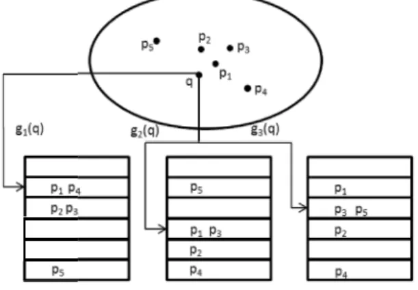
Fig. 1 presents an examp ed into three hash tables co
q, by checking the three buc By ranking their distances t
The main drawback of th ber of hash tables to cover are needed to achieve 1.1-a used in [4]. Thus, the whol the number of hash tables LSH [15] was proposed. Multi-probe LSH. The ma ly derived probing sequenc nearest neighbors of a quer the number of needed hash
Fig. 2. Distan
Multi-probe LSH is bas et al.[7] described above, r the authors first define a ha and M is the number of h basic LSH method checks
ple of 2-NNS, where L = 3. Objects p1, p2, …, p5 are ins
orresponding to hash functions g1, g2, g3. For a given qu
ckets g1(q), g2(q), g3(q), we get the candidates p1, p3, p4,
to q, we return p1 and p3as the 2-NN objects.
Fig. 1. LSH index structure
he above index structure is that it may require a large nu most nearest neighbors. For example, over 100 hash tab approximation in [9], and as many as 583 hash tables le data structure takes too much space. In order to red s while keeping a good approximation ratio, Multi-pr
ain idea of the Multi-probe LSH method is to use a care ce to check multiple buckets that are likely to contain ry object. Since each hash table provides more candida
tables could be reduced.
nce from q to the boundary of its neighbor bucket
sed on the family of locality-sensitive functions of Da returning integer values. To derive the probing sequen sh perturbation vector Δ = {δ1, …, δM} where δiϵ {-1, 0
hash functions for each hash table. Given a query q, the hash bucket g(q) = (h1(q), h2(q), … , hM(q)), wh
sert-uery , p5. um-bles are duce robe eful-the ates, atar nce, , 1} the hile
Multi-probe LSH checks also the buckets g(q) + Δ1, g(q) + Δ2, …, g(q) + ΔT. These
buckets are ordered according to their “success probability” which is a score estimat-ed using formula score(Δ) = ∑ ( ) , where ( ) is the distance from q to the boundary of the bucket hi(q) + δi. For example, in Fig. 2, xi(1) is the distance from q to the boundary of the bucket hi(q) + 1, where hi(q) = (ai· q +bi)/W and fi(q) = ai· q +bi.
Multi-probe LSH is originally designed as an in-memory algorithm. In this paper, however, we consider that the multidimensional vectors are stored in a secondary storage such as hard disk. The problem with Multi-probe LSH in this new context is that many probes are needed for each hash table and the probed buckets are randomly stored in the disk, so a lot of I/Os are required for each query. Our objective in this paper is to reduce the number of I/Os for a K-NN search.
Other Related Work. LSH Forest indexing method [1] represents each hash table by a prefix tree to eliminate the need of finding the optimal number of hash functions per table. However, this method does not help reduce the number of hash tables, so the space consumption and query time are not improved. There exists some other work which tends to estimate optimal parameters with sample datasets [8], use improved hash functions [11], [13], [17], [18] or divide the dataset into clusters before building LSH indexes [16]. All these methods are complementary to the Multi-probe LSH and our improved structure and could be combined with our method in order to achieve better performance and quality.
3
Dynamic Multi-probe LSH
3.1 OverviewThe main idea of DMLSH is to dynamically vary the granularity of buckets in order to adapt the number of objects they contain to the size of a disk page. We use the same locality-sensitive hash functions and the same probing sequence as Multi-probe LSH. More precisely: 1) Instead of directly building a hash table by using all M func-tions, we first build a hash table by using only one LSH function. If a bucket contains more than l objects (where l is the number of objects contained in a disk page), we add a second LSH function to this bucket in order to split it into several small buckets. If some small bucket still contains more than l objects, we continue adding LSH func-tions until each bucket contains less than l objects or the number of functions used becomes to be M. We store the signatures of all these buckets in to a B+ tree. Note that these signatures have different lengths, so the keys in the B+ tree have variable size. 2) We use the sequence probing algorithm of Multi-probe LSH to generate the signatures of the buckets to be probed. If the bucket signature exists in the B+ tree index, we will take the objects in the corresponding bucket as candidates; otherwise, we will check the bucket whose signature is a prefix of the generated signature.
Let us explain these principles through an example. In Fig. 3(a), a basic LSH table has been built using 2 hash functions h1 and h2. For a given query q, if we use
01, 10, 00, 21 and 20. It m candidates. In Fig. 3(b), in function h1 first, then only
(in this example l=2), we a query q, we use the algorit sequence, i.e. 11, 01, 10, 00 (e.g. 11), we take the buck 11). Thus, the probing sequ be accessed. (a) Basic LSH Fig. 3.2 Index Construction As in the Multi-probe LSH ly generate M LSH functio LSH is that not every insert the hash results are stored i search that we do in the B+ of the searched key, for exa result. Thus, we have slight Note that signatures (keys) digit is an integer value re only consider binary digits. DMLSH Tree. We call DM signatures of the buckets pr information about these bu DMLSH tree.
The only modification th is that we overloaded the co operators “==”, “<” and “>”
• Given two keys k1
the other one (inclu
means that, we need to access 6 pages on the disk to ge nstead of using directly 2 hash functions, we use one h
if the number of objects in a bucket exceeds a thresho add a second hash function for this bucket. For the sa thm of the Multi-probe LSH to generate the same prob 0, 21 and 20. For a signature that corresponds to no buc ket whose signature is its prefix (i.e. bucket 1 for signat uence becomes 1, 01, 00 and 2. Only 4 disk pages need
(b) DMLSH . 3. Dynamically adding hash functions
n
, we use L hash tables, and for each hash table we rando ons. The difference between our method and Multi-pr
ted object needs to be hashed with all the M functions, in a B+ tree rather than a normal hash table. However, + tree is not an exact match. Instead, we may return a pre ample, when searching for 001010, we may return 001 a tly modified the search algorithm of the traditional B+ tr ) stored in the B+ tree are sequences of “digits”, wher eturned by an LSH function. For simplicity, our examp
MLSH tree the specific (in memory) B+ tree that stores roduced by the DMLSH method, together with some ex uckets. Note that only non-empty buckets are stored i hat we have made to the B+ tree algorithm described in omparison operators of the keys. The new definitions of
” are as follows:
and k2, we say that k1 == k2 if one of k1 or k2 is a prefix
uding the case where k1 = k2 as sequences).
et 7 hash old l ame bing cket ture d to om-robe and the efix as a tree. re a ples the xtra in a n [6] f the x of
• If k1 == k2 is not t d1 + s1 and k2 = k
empty) and d1, d2a
tively k1 > k2) if d1
For example, we have 001 = The following property h
signatures k1 and k2 produc
Proof. Let us suppose t have k1 == k2 with e.g. k1b
included into the one of si buckets issued from DMLS Since it is not possible to h “<” and “>” operators pres tures produced by DMLSH Each hash table is main (hash value) of each non-e into the tree. Each key in th 1. a counter for the num
nb_hashes_used;
2. a counter for the number 3. the address of the page c 4. a set HV containing the
functions.
Fig. 4. D
Construction of the DML construction. For each of th an initial empty DMLSH tr each of the DMLSH trees w
Algorithm 1. Con for i = 1 to L do for j = 1 to M Genera end for Create an em end for foreach v ϵ S do InsertVector end for
true, it is easy to show that k1 and k2have the form k1 = k + d2 + s2, where k, s1, s2 are digit sequences (possi
are single digits, with d1 != d2. We say that k1 < k2 (resp 1 < d2 (respectively d1 > d2).
== 00101, 0101 < 011 and 10110 > 100010, etc. holds for DMLSH bucket signatures: For any two dist ced by DMLSH, we have either k1 < k2 or k1 > k2.
that for two distinct signatures produced by DMLSH being a prefix of k2. In this case, the bucket of signature k
ignature k1. But this is in contradiction with the fact t
SH produce a partitioning of the multidimensional spa have k1 == k2, we deduce from the properties of the “=
sented above that k1 < k2 or k1 > k2. Consequently, sig
respect a strict total order induced by the “<” operator. ntained as a DMLSH tree as follows: the bucket signat empty bucket is treated as a key and the keys are inser he leaf node is followed by (Fig. 4):
mber of hash functions used for getting this signatu r of vectors in the corresponding hash bucket, nb_vector
containing these vectors, @;
hash values of these vectors computed by using all the
Data structure of each item in the leaf nodes
LSH Index. Algorithm 1 shows the process of the in he L hash tables, we generate M random LSH functions ree. Then, for each vector v in the database S, we insert v
with InsertVector (Algorithm 2).
nstruction of the index structure M do
ate a random LSH function hi,j
mpty DMLSH tree Treei
r(v) (Algorithm 2) k + ibly pec-inct we k2 is that ace. ==”, gna-ture rted ure, rs; e M ndex and v in
As shown below, vector insertion respects the DMLSH strategy to generate new buckets that use as few hash functions as possible. Only when the size of a bucket exceeds a threshold, we add a new hash function for this bucket and distribute the objects into smaller buckets. When the number of hash functions used becomes to be
M, we stop adding new hash functions and we will store the newly inserted objects in the overflow pages of the full bucket.
Object Insertion. As shown in Algorithm 2, when inserting a new vector v, we insert it into each of the L hash tables. For each hash table, we compute the hash value g(v)
of vector v, using the M functions, and search the key g(v) in the corresponding B+ tree. If a prefix of g(v) exists in the tree, the function Treei.find(g(v)) will return the
item in the leaf node which corresponds to the prefix key. Note that a prefix may not exist in the tree, because empty buckets are not stored in the B+ tree. If there is no prefix of the searched key, item is NULL and we will add into the tree a new item with the shortest prefix of g(v) which is not a prefix of any other existing key. This is done by function Treei.insert(g’(v), item). The length of this prefix is computed by
function Nb_hash (Algorithm 3). Finally, we insert the vector into the bucket page linked to the found (or inserted) prefix key and update the other fields of the leaf item with AddVectorToItem (see Algorithm 4).
Algorithm 2.InsertVector(v): insert a vector v
for i = 1 to L do
g(v) = (hi,1(v), hi,2(v), …, hi,M(v))
item = Treei.find(g(v))
if item == NULL then item = New_leaf_item()
nb_hashes_used = Nb_hash(v, i) (Algorithm 3) g’(v) = (hi,1(v), hi,2(v), …, hi,nb_hashes_used(v))
Treei.insert(g’(v), item)
AddVectorToItem(v, item, i) (Algorithm 4) end for
Algorithm 3.Nb_hash(v, i): determine nb_hashes_used for vector v
in Treei
g(v) = (hi,1(v), hi,2(v), …, hi,M(v))
pred = Treei.find_pred(g(v))
succ = Treei.find_succ(g(v))
lcc_pred = length(longest_common_prefix(pred, g(v))) lcc_succ = length(longest_common_prefix(succ, g(v))) lcc = max(lcc_pred, lcc_succ)
return lcc+1;
Algorithm 3 shows how to determine the number of hash functions to use for a newly inserted vector whose complete hash value does not have a prefix key in the
tree. We first compute the key g(v) using all M hash functions, then we search in the tree for pred which is the greatest key smaller than g(v) and succ which is the smallest key larger than g(v). The next step is to compute lcc which is the maximum length of the longest common prefix between g(v) and pred/succ. Note that if pred or succ do not exist, the corresponding length of the common prefix is 0. At the end, we return
lcc+1 as the number of hash functions to be used.
Algorithm 4 shows how to add a vector v into an item. Insertion is possible only if the counter nb_vectors is below the threshold l (l = B/sizeof(v), where B is the size of a disk page), or if the maximum number M of hash functions is reached. Insertion adds v into the page @ (or into an overflow page) and the full signature g(v) to HV. If insertion is not possible, the bucket is “split” as follows: its item is removed from the B+ tree and all its vectors are reinserted in buckets using one more hash function (Algorithm 5). If the bucket containing the reinserted vector already exists in the tree, the vector is directly inserted; otherwise, a new bucket is created.
Algorithm 4.AddVectorToItem(v, item, i): add a vector v into a leaf
entry item of Treei
if item.nb_vectors < lor item.nb_hashes_used==M then item.nb_vectors++
g(v) = (hi,1(v), hi,2(v), …, hi,M(v))
Add g(v) into item.HV
Add v into the page at address item.@ or into an overflow page else
Treei.remove(item)
for each vjϵ item do
ReinsertVector(vj, item.nb_hashes_used+1, i)
end for
Algorithm 5.ReinsertVector(v, k, i): reinsert vector v into Treei with
k hash functions
g(v) = (hi,1(v), hi,2(v), …, hi,k(v))
item = Treei.find(g(v))
if item== NULL then item = New_leaf_item() item.nb_hashes_used = k Treei.insert(g(v), item)
end if
AddVectorToItem(v, item, i) (Algorithm 4)
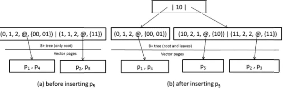
Example. Since the insertion algorithm is the same for all the hash tables, we only consider one hash table as an example. For simplicity, we assume the threshold l = 2 and the maximum number of hash functions M = 2. Initially, we have four objects p1, p2, p3 and p4, with h1(p1) = 0, h1(p2) = 1, h1(p3) = 1 and h1(p4) = 0. Their complete hash
values are stored in the set 5(a). The format of the elem object p5 with h1(p5) = 1, g(
3 which is larger than l, so tion h2). We reinsert all the
with keys 10 and 11 are ins for key 0, the bucket is not
F
3.3 Approximate K Ne Algorithm. For a given que tables. We build an empty signatures of the accessed b (Section 3.2.1), but its item value of q using all M hash probing sequence for g(q). found in [15]. We note T th
For each probe, we searc means that the bucket has a search the probed key in th in the set HV, this means th into the “physical” bucket o linked to pk into the candida
After retrieving all the ca ry q, rank them in increasin Example. Let us consider 10, T = 3 and the generated find the signature in the tree 10 into Probed_Tree. For th
HV set (00 ϵ {00, 01}), we 0 into Probed_Tree. For
Probed_Tree, meaning that
extra I/O for this probe. In buckets, we only loaded 2 p
HV following the prefix keys. The index is shown in F ment in the leaf nodes is defined by Fig. 4. When we in
(p5) = 10, the counter nb_vectors for the bucket 1 becom
we need to split this hash bucket (i.e. add one hash fu objects of bucket 1. Fig. 5(b) shows the result: new ent serted in the B+ tree and the old entry with key 1 is delet
split.
Fig. 5. Example of a DMLSH index
arest Neighbor Search
ery q, we repeat the following process for each of the h y B+ tree Probed_Tree in memory, used to memorize buckets. This tree has the same properties as a DMLSH t ms only contain a bucket signature. We compute the h h functions, i.e. g(q) = (h1(q), …, hM(q)) and generate
The algorithm of generating the probing sequence can he number of probes.
ch the probed key in Probed_Tree. If its prefix is found already been checked, so we skip this probe. Otherwise, he DMLSH tree. If a prefix key pk is found and g(q) ex
hat the bucket of signature g(q) is not empty and is inclu of signature pk. Therefore, we add the vectors in the page
ate set and insert pk into Probed_Tree.
andidates, we compute the distances from them to the q ng order of their distances and return the top-k results.
the example in Fig. 5(b). Suppose g(q) = (h1(q), h2(q)
d probing sequence is 10,00,01. For the first probe 10, e, we load the linked page, add p5 as a candidate and in
he second probe 00, we find its prefix 0. Since 00 is in load the linked page, add p1 and p4 as candidates and in
the last probe 01, we find its prefix 0 in the t t the bucket has already been probed, so we don’t need this example, instead of loading 3 pages for the 3 pro pages. Fig. nsert mes unc-tries ted; hash the tree hash the n be d, it we xists uded e(s) que-)) = we nsert the nsert tree d an obed
Properties. The DMLSH method proposed in this paper has two important properties compared to the original Multi-Probe LSH. P1: Under the same parameter setting, the number of I/Os made by DMLSH for a given query q is no more than that made by Multi-probe LSH. P2: Under the same parameter setting, the accuracy of the K-NN search made by DMLSH for a given query q is not lower than that of Multi-probe LSH. They could be easily proved theoretically, since in DMLSH, 1) several non-full probed buckets may share the same prefix key and they are stored in a single disk page; 2) the candidate set is a superset of that produced by MLSH.
4
Experimental Evaluation
4.1 Methods under EvaluationDMLSH is an I/O efficient version of Multi-probe LSH, so we will compare these two methods by varying the different parameters: the number of hash functions M, the number of hash tables L and the number of probes T.
Our method could be also combined with basic LSH and its variants mentioned in related work, by organizing each hash table as a DMLSH tree. However, the impact in this case is less important than with Multi-probe LSH, because a single bucket is ac-cessed in each table; also these methods have less practical utility because of the high number of tables. Consequently, we limit our study to the more effective Multi-probe LSH method.
4.2 Dataset
We choose two datasets for our experimental evaluation, widely used in the related work. They are: Color Data. The Color dataset contains 68040 vectors of 32 dimen-sions, which are the color histograms of images in the Corel collection1. The dimen-sion values are real numbers with at most 6 decimal digits ranging from 0 to 1.We randomly choose 100 vectors as query examples. Audio Data. The audio dataset contains 54387 vectors of 192 dimensions. It is extracted from the LDC SWITCHBOARD-1 collection2. The values are real numbers between -1 and 1. We increase the size of both datasets to be 1 million by inserting noise vectors for the
following experiments. We randomly choose 100 vectors as query examples.
4.3 Evaluation Metrics
We adopt two metrics to measure our method: query efficiency and query accuracy. Since the space consumption of our method is about the same with Multi-probe LSH, we do not consider this metric.
Query Efficiency. Since the vectors are stored in the secondary storage, we evaluate the query efficiency in terms of I/O cost. In the experiments, we set the page size as
1http://kdd.ics.uci.edu/databases/CorelFeatures/ 2
the size of 100 vectors. Note that DMLSH introduces a CPU overhead for distance computation, since the number of candidates it produces is larger than for MLSH. However, the measures in this case indicate only a small difference (5%), not signifi-cant compared with the I/O saving.
Query Accuracy. We measure the average recall ratio of the 100 K-NN queries for
K=20. Given a query object q, let E(q) be the set of exact K-NN objects, and F(q) the set of found K-NN objects. Then the recall ratio is defined as follows:
Recall = | ( )∩ ( )|| ( )| (1)
4.4 Experimental Results
In this section, we compare DMLSH and MLSH by varying the number of hash func-tions M, the number of hash tables L, respectively the number of probes T.
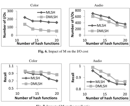
Impact of the Number of Hash Functions M. We measured the I/O cost and the recall ratio of the first two methods by varying the maximum number of hash func-tions (M) used for each hash table. For both datasets, the number of hash tables L is set to 3 and the number of probes T is set to 100. The results are shown in Fig. 6 and Fig. 7.
Color Audio
Fig. 6. Impact of M on the I/O cost
Color Audio
Fig. 7. Impact of M on the recall ratio
0 100 200 300 10 15 20 Number of I/ O s
Number of hash functions
MLSH DMLSH 0 200 400 600 800 10 15 20 Number of I/ O s
Number of hash functions
MLSH DMLSH 0.5 0.7 0.9 1.1 10 15 20 Recal l
Number of hash functions
MLSH DMLSH 0.8 0.9 1 10 15 20 Recal l
Number of hash functions
MLSH DMLSH
For the Color dataset, we set W = 0.6. DMLSH reduces the I/O cost by 39% - 67% and increases the recall ratio by 3% - 23%. For the Audio dataset, we set W = 3.5. DMLSH reduces the I/O cost by 13% - 25% and increases the recall ratio by 3% - 6%.
We can see that the overall trend is that, when the number of hash functions grows, both the I/O cost and the recall ratio decrease. This is because when we add a new hash function, 1) the average size of each bucket is decreased and 2) more empty buckets are probed.
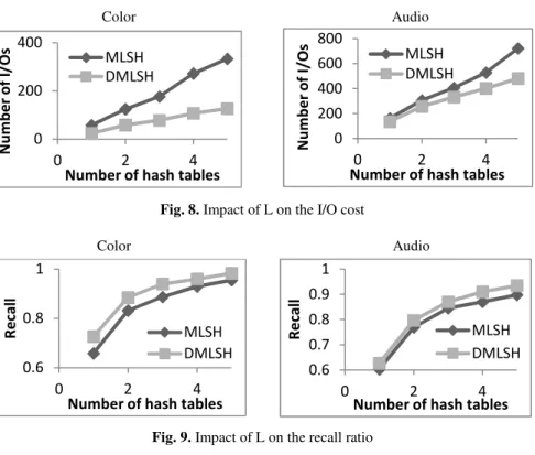
Impact of the Number of Hash Tables L. Fig. 8 and Fig. 9 show the impact of the number of hash tables L on the I/O cost and on the recall ratio. The number of probes
T is set to 100.
For the Color dataset, we set M = 14 and W = 0.6. DMLSH reduces the I/O cost by 53% - 62% and increases the recall ratio by 3% - 10%. For the Audio dataset, we set
M = 18 and W = 3.5. DMLSH reduces the I/O cost by 16% - 33% and increases the recall ratio by 1% - 9%.
Color Audio
Fig. 8. Impact of L on the I/O cost
Color Audio
Fig. 9. Impact of L on the recall ratio
When the number of hash tables grows, both the I/O cost and the recall ratio in-crease. This is normal, because when we use L+1 hash tables, the set of candidates is always a superset of that produced by using L hash tables. The choice of the number of hash tables is a trade-off between query efficiency, query accuracy and space consumption.
We observed that, to achieve the same recall ratio, our method DMLSH needs fewer hash tables than MLSH, hence consumes less space.
0 200 400 0 2 4 Number of I/ O s
Number of hash tables
MLSH DMLSH 0 200 400 600 800 0 2 4 Number of I/ O s
Number of hash tables
MLSH DMLSH 0.6 0.8 1 0 2 4 Recal l
Number of hash tables
MLSH DMLSH 0.6 0.7 0.8 0.9 1 0 2 4 Recal l
Number of hash tables
MLSH DMLSH
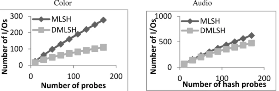
Impact of the Number of Probes T. In Fig. 10 and Fig. 11, we vary the number of probes from 10 to 170. For both datasets, the number of hash tables L is set to 3.
For the Color dataset, we set M = 14 and W = 0.6. DMLSH reduces the I/O cost by 33% - 60%. The bigger the number of probes, the higher the reduction of I/O cost. With the same number of probes, DMLSH increases the recall ratio by 4% - 16%. For the Audio dataset, we set M = 18 and W = 3.5. DMLSH reduces the I/O cost by 2% - 24% and increases the recall ratio by 3% - 5%. To achieve the same recall ratio, our method DMLSH needs fewer probes than MLSH.
Color Audio
Fig. 10. Impact of T on the I/O cost
Color Audio
Fig. 11. Impact of T on the recall ratio
5
Conclusion
This paper presents the Dynamic Multi-probe LSH indexing method, which is a more I/O efficient version of the Multi-probe LSH. It dynamically varies the granularity of buckets in order to adapt the number of objects they contain to the size of a disk page. For the construction of the index, it uses initially one hash function and adds a new hash function only when the bucket size exceeds the page size. In the final hash table, the buckets are built by using a different number of hash functions; consequently they have signatures of different length. Bucket signatures are indexed by a slightly modi-fied B+ tree to accelerate the search speed.
0 100 200 300 0 100 200 Number of I/ O s Number of probes MLSH DMLSH 0 500 1000 0 100 200 Number of I/ O s
Number of hash probes
MLSH DMLSH 0.6 0.8 1 0 100 200 Recal l Number of probes MLSH DMLSH 0.6 0.8 1 0 100 200 Recal l
Number of hash probes
MLSH DMLSH
For a given query, we first generate the probing sequence and then we access the probed buckets. Since several probed buckets may share the same prefix key and are stored in the same physical page, we need only one single I/O to access these buckets. Thus, the total number of disk accesses is reduced. In addition, since the candidate set is a superset of that produced by Multi-probe LSH, the recall ratio of the approximate
K-NN query results is always higher than or equal to that of the Multi-probe LSH.
References
1. Bawa, M., Condie, T., Ganesan, P.: Lsh forest: self-tuning indexes for similarity search. In: WWW, pp. 651–660 (2005)
2. Bentley, J.L.: Multidimensional binary search trees used for associative searching. Com-munications of the ACM 18(9), 509–517 (1975)
3. Berchtold, S., Keim, D.A., Kriegel, H.P.: The X-Tree: an index structure for high-dimensional data. In: Proceedings of the 22nd VLDB Conference, pp. 28–39 (1996) 4. Buhler, J.: Efficient large scale sequence comparison by locality-sensitive hashing.
Bioin-formatics 17, 419–428 (2001)
5. Ciaccia, P., Patella, M., Zezula, P.: M-tree an efficient access method for similarity search in metric spaces. In: Proceedings of the 23rd VLDB Conference, pp. 426–435 (1997) 6. Comer, D.: The ubiquitous B-tree. ACM Computing Surveys 11(2), 121–137 (1979) 7. Datar, M., Immorlica, N., Indyk, P., Mirrokni, V.S.: Locality-sensitive hashing scheme
based on p-stable distributions. In: Proceedings of the Twentieth Annual Symposium on Computational Geometry, pp. 253–262 (2004)
8. Dong, W., Wang, Z., Josephson, W., Charikar, M., Li, K.: Modeling LSH for performance tuning. In: CIKM 2008, pp. 669–678 (2008)
9. Gionis, A., Indyk, P., Motwani, R.: Similarity search in high dimensions via hashing. In: Proceedings of the 25th Very Large Database (VLDB) Conference, pp. 518–529 (1999) 10. Guttman, A.: R-Trees: A dynamic index structure for spatial searching. In: Proceedings of
the ACM SIGMOD International Conference on Management of Data, pp. 47–57 (1984) 11. He, J., Liu, W., Chang, S.: Scalable similarity search with optimized kernel hashing. In:
ACM SIGKDD, pp. 1129–1138 (2010)
12. Indyk, P., Motwani, R.: Approximate nearest neighbor: towards removing the curse of di-mensionality. In: Proceedings of STOC, pp. 604–613 (1998)
13. Jegou, H., Amsaleg, L., Schmid, C., Gros, P.: Query adaptative locality sensitive hashing. In: ICASSP 2008, pp. 825–828 (2008)
14. Katayama, N., Satoh, S.: The SR-tree: an index structure for high-dimensional nearest neighbor queries. In: SIGMOD Conference, pp. 369–380 (1997)
15. Lv, Q., Josephson, W., Wang, Z., Charikar, M., Li, K.: Multi-probe LSH: efficient index-ing for high-dimensional similarity search. In: Proceedindex-ings of the 33rd International Con-ference on Very Large Data Bases (VLDB), Vienna, Austria, pp. 950–961 (2007)
16. Pan, J., Manocha, D.: Bi-level locality sensitive hashing for k-Nearest Neighbor computa-tion. In: ICDE, pp. 378–389 (2012)
17. Raginsky, M., Lazebnik, S.: Locality-sensitive binary codes from shift-invariant kernels. In: Advances in Neural Information Processing Systems, pp. 1509–1517 (2009)
18. Satuluri, V., Parthasarathy, S.: Bayesian locality sensitive hashing for fast similarity search. PVLDB 5(5), 430–441 (2012)
19. Weber, R., Schek, H., Blott, S.: A quantitative analysis and performance study for similari-ty-search methods in high-dimensional spaces. In: VLDB, pp. 194–205 (1998)