Durham Research Online
Deposited in DRO:
28 September 2018
Version of attached le:
Accepted Version
Peer-review status of attached le:
Peer-reviewed
Citation for published item:
Xu, Jiangjiao and Sun, Hongjian and Dent, Chris (2018) 'ADMM-based distributed OPF problem meets stochastic communication delay.', IEEE transactions on smart grid. .
Further information on publisher's website:
https://doi.org/10.1109/TSG.2018.2873650 Publisher's copyright statement:
c
2018 IEEE. Personal use of this material is permitted. Permission from IEEE must be obtained for all other uses, in any current or future media, including reprinting/republishing this material for advertising or promotional purposes, creating new collective works, for resale or redistribution to servers or lists, or reuse of any copyrighted component of this work in other works.
Additional information:
Use policy
The full-text may be used and/or reproduced, and given to third parties in any format or medium, without prior permission or charge, for personal research or study, educational, or not-for-prot purposes provided that:
• a full bibliographic reference is made to the original source
• alinkis made to the metadata record in DRO
• the full-text is not changed in any way
The full-text must not be sold in any format or medium without the formal permission of the copyright holders. Please consult thefull DRO policyfor further details.
Durham University Library, Stockton Road, Durham DH1 3LY, United Kingdom Tel : +44 (0)191 334 3042 | Fax : +44 (0)191 334 2971
ADMM-based Distributed OPF Problem Meets
Stochastic Communication Delay
Jiangjiao Xu,
Student Member, IEEE, Hongjian Sun,
Senior Member, IEEE,
Chris Dent,
Senior Member, IEEE
Abstract—An increasing number of distributed generators (DGs) will penetrate into the distribution power system in future smart grid, thus a centralized control strategy cannot effec-tively optimize the power loss problem in real-time. This paper examines the idea of a fully distributed Optimal Power Flow (OPF) approach, based on the alternating direction multiplier method (ADMM), to optimize the power loss. The objectives are not only to effectively obtain the minimization of power loss, but also to analyze the effect of communication time-delay on optimization performance. Both synchronous and asynchronous iterative algorithms are proposed to study the convergence results. In addition, four different strategies are proposed to improve convergence speed when delay occurs. The proposed weighted autoregressive (AR) strategy can reduce the fluctuation effectively. In comparison with synchronous algorithm, simula-tion results show that the asynchronous algorithm has a better optimization result.
Index Terms—Altering direction method of multiplier (ADMM), Optimal Power Flow (OPF), reactive power control, time-delay analysis, synchronous and asynchronous algorithms.
I. INTRODUCTION
T
HE large penetrations of DGs in distribution grid could benefit to the power system, for example, increasing energy diversity, improving reliability and reducing environ-mental pollution. Meanwhile, these DGs can provide a large quantity of ancillary services that are of great interest to the optimization of the grid [1], [2].Reactive power services play an important role, i.e., satisfy the requirement of reactive power load, control bus voltage in a system wide, decrease the network loss, relieve the transmission block and provide sufficient reserve to ensure the security of system in emer-gency.The development of smart grid requires Information and Communication Technologies (ICT) architecture to maximise the systems potential. In order to realize the autonomous control in real-time, a distributed optimization strategy will combine the ICT to implement the control and optimization.A great mass of techniques have been investigated for control and optimization in electrical power system [3]. The allocation of reactive power had been designed to solve OPF problems since the 1960s [4] and a number of optimization techniques had been proposed in recent decades [5]–[8]. However, these centralized approaches, based on offline tech-niques, required an accurate network structure and operation conditions in advance. In addition, optimization procedure required a highly reliable communication process and also produced a large communication and computation delay. For these reasons, these approaches are not able to do real-time monitoring and control.
To overcome this shortcoming, a variety of distributed strategies which could achieve real-time optimization had been proposed. The concept of consensus fashion in a distributed system can be found in [9].The partial distributed algorithms, which separated the distribution network into several areas, were studied in [10]–[13]. In [10] a fast decomposition opti-mization scheme using the interior point OPF was proposed that the decomposition scheme was effective. Reference [11] introduced a distributed semi-definite programming (SDP) relaxation technique which guaranteed the faster convergence speed to obtain solution. A primal and a dual algorithm was propsoed in [12] to coordinate the subproblems de-composed from the convexified OPF, the computation time could be improved dramatically. Reference [13] discusses three ADMM-based distributed optimization algorithms for solving the dynamic DC-OPF problem with DR. The nu-merical case studies present solution accuracy, convergence performance and communication requirement of the three proposed distributed algorithms. However, these distributed approaches just divided the network into several areas. The problems in centralized approaches still existed because of the distance between two local controllers and requirement of reliable communication. In contrast, distributed algorithms were investigated to work out the distributed OPF problem. An example of full distributed approach in [14] utilized a distributed scheme to control the reactive power and a genetic algorithm (GA) was adopted to optimize objectives. However, the proposed optimization process of GA was time-consuming with respect to the requirements of real-time control [15]. Reference [16] capitalized the ADMM to allocate the reactive power to minimize the system power loss which showed a better convergence speed compared to the dual-ascent ap-proach. And [17] also provided the ADMM method to solve the consensus optimization problem, the results demonstrated an expedited convergence speed. In addition, asynchronous ADMM algorithm in [18] based on the distributed convex optimization problem is provided to simulate the convergence results. The simulations confirm the convergence of proposed asynchronous algorithm.These proposed distributed strategies still required a certain limited information exchange. However, they did not analyze the potential effect of time-delay. When the communication delay is considered, some algorithms may not obtain the optimal target and sometimes cannot converge properly.
The ADMM approach, which is an augmented Lagrangian-based algorithm, is a popular choice due to the robust and fast convergence results both in theory and practice [19].
In addition, ADMM is well suited to distributed optimiza-tion and in particular to large-scale power system. However, when time-delay is considered in the ADMM algorithm, the synchronization will become a critical problem. Although the synchronization of all nodes enables the algorithm to be effectively controlled, the communication time in a syn-chronous algorithm will be limited due to the slowest node’s communication transmission. A few papers [20]–[22] have introduced communication time-delay system into the dis-tributed ADMM algorithm, which was based on a master-slave strategy. Reference [20] presents an asynchronous dis-tributed algorithm by using ADMM to study convergence rate and accuracy of consensus algorithm. The simulation results considering time-delay show possible numerical instabilities and sensitivities of the convergence rate on different strategies. An asynchronous algorithmic framework based on ADMM is proposed to perform convergence with information exchange in [21]. The experimental studies demonstrate convergence performance for both synchronous and asynchronous schemes with communication delay. And [22] studied the linear con-vergence conditions of asynchronous ADMM method. The results reveal the impact of different parameters, network delay and network size on the convergence performance. The proposed algorithms in these papers could still be treated as a centralized control approach, because the master required to collect information from all other independent workers. Only when all the information was received by the master, the master would broadcast other nodes to proceed the next step.
The literatures above do not discuss a fully distributed OPF problem with stochastic communication delay in a distribu-tion network. The majority of recent papers also have not investigated this particular problem with both synchronous and asynchronous time-delay models. Although The asynchronous model means that each node could operate its own iterative step without considering the time synchronization problem. This paper proposes a feasible fully distributed approach to optimize the allocation of reactive power. The novelty of this paper is to analyze the effect of communication time-delay on the performance of both synchronous and asynchronous algorithms. The main contributions of this work are as follows:
• A distributed approach with a limited coordination of neighbouring nodes is studied to solve the optimization problem. An improved iterative step of ADMM algorithm is used to analyze the convergence result. Compared with the widely-used master-slave model, the distributed model can reduce the requirements of reliability of communication system. Both synchronous and asynchronous algorithms that consider communication time-delay model are discussed in this paper. The simulation results prove that a small probability of communication delay has a significant influence on the results of distributed ADMM algorithm. Comparing with the synchronous algorithm, the proposed asynchronous algorithm has a better convergence speed and optimization results during the same wall clock time period.
• As the fluctuation in experimental results with time-delay, we proposed four strategies, such as, skipping strategy (SS), previous value strategy (PVS), autoregressive strategy
(ARS) and weighted AR strategy (WARS), to perform the syn-chronous and asynsyn-chronous convergence results. The proposed WARS can effectively reduce the fluctuation and improve the convergence results for both synchronous and asynchronous algorithms with different delay probabilities.
The rest of the paper is structured as follows: in Section II, the distribution network model with communication is described, then the centralized power loss problem formula is presented. Section III provides the synchronous and asyn-chronous algorithms with end-to-end communication time-delay model, and four different iterative strategies are proposed to assess the convergence results. The simulation results are shown in Section IV. Section V draws conclusions and dis-cusses future work.
II. NETWORK MODEL AND PROBLEM FORMULATION
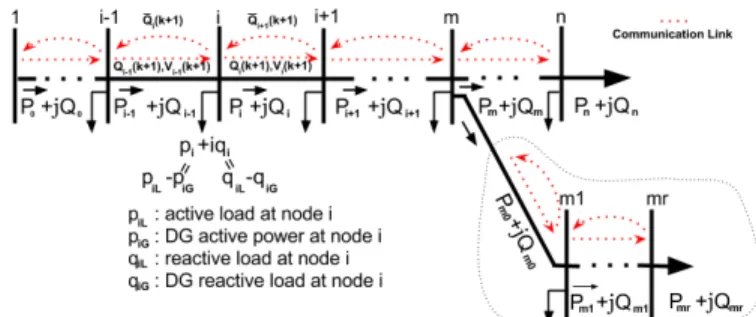
Fig. 1:
One-line main feeder with a lateral branching
network.
Fig. 1 shows one-line main feeder including a lateral branch distribution network with the description of the notations and also displays communication links for the information exchange. It is a bi-direction communication between neigh-bouring nodes. We define ν and β as the set of nodes and branches, respectively. (i,j)∈βmeans nodesi,jare neighbour nodes.
For a ladder network, the distribution flow equations can be written as [23] s.t. ∀ i∈ν Pi+1=Pi−ri Pi2+Q2i V2 i −pi+1 (1a) Qi+1=Qi−xi P2 i +Q2i V2 i −qi+1 (1b) Vi2+1=Vi2−2(riPi+xiQi) +Ri (1c) |Si−1|≤Simax−1 . (1d)
wherePi andQi are the active and reactive power flow from
nodeitoi+ 1, respectively.Vi is the voltage level at nodei.
riandxi are the branch resistance and reactance from nodei
toi+ 1, respectively.pi+1andqi+1are the active and reactive power at nodei+ 1, respectively.Ri= (ri2+x2i)
Pi2+Q2i V2
i
pi+1 andqi+1consist of local consumption minus generation, for example
pi+1=piL−piG (2a)
qi+1=qiL−qiG (2b)
To meet the requirements of real-time OPF, it is assumed that the active power output in this paper is constant during the optimization procedure. We assume that piL,piGandqiL are
fixed and only DG’s reactive power termqiGcan be regulated
within limits. For initial node 1, terminated nodes n andm, V1 is constant andPn=Pmr =Qn =Qmr = 0.
Our target is to minimize the global optimization problem which is system total active power loss in this paper. The global objective function within multiple nominal operational constraints can be written
min power loss z }| { X i∈ν (Fi(Qi)) =X i∈ν ri Pi2+Q2i V2 i (3a) s.t. ∀i∈ν |Qi−Qi−1−qiL+Qlosi−1|≤si (3b) Vimin≤Vi≤Vimax (3c) Vi2=Vi2−1−2(ri−1Pi−1+xi−1Qi−1) +Ri−1 (3d) |Si−1|≤Simax−1 . (3e)
where (3a) is the total power loss function. Qlosi−1 =
xi−1
P2 i−1+Q2i−1
V2 i−1
. (3b) is the power balance constraints, si is
the maximum apparent power capacity of inverters of DG. For nodes without DG, si = 0. The maximum value can
be determined by the maximum value of converter voltage and maximum current rating of converter [24]. (3c) is the voltage level constraints. Vmin
i ,Vimax are the minimum and
maximum voltage magnitude of node i, respectively. We set Vmin
i = 0.95, Vimax = 1.05 according to the American
National Standard ANSI C84.1-2011. (3d) is the voltage con-straints between two adjacent nodes. (3e) is the transmission line capacity constraints,Simax−1 denotes the maximum apparent power of branch transmission line from nodei−1toi.
Since consensus ADMM is assured to converge only in convex scenarios, and OPF is a non-convex problem, the distributed solution is in general not guaranteed to converge. It is necessary to derive the linear approximant of the power flow equations (3). Under normal circumstances, the amount of voltage variation from node to node is relatively small com-pared to the rated voltage level. Hence, we assumeVi−1≈V1 that is a constant value, and also approximate (3a) and (3d) to a linear constraint (4a) and (4d), respectively.The optimization function can be approximated as a linear quadratic function in this paper [25], [26]. minX i∈ν ri P2 i +Q2i V2 1 (4a) s.t. ∀i∈ν |Qi−Qi−1−qiL|≤si (4b) Vimin≤Vi≤Vimax (4c) Vi=Vi−1−2 (ri−1Pi−1+xi−1Qi−1) V1 (4d) |Si−1|≤Simax−1 . (4e)
In [25] and [26], the simulation results show that the linear power flow equations are well justified for a wide range of distribution networks. This observation is powerful because the linear power flow equations in (4) are convex. Convexity means that the optimization solution can be achieved effi-ciently and each node can communicate with a central au-thority.In this paper, we focus on the distributed optimization algorithm to solve the problem, which only communicate information between neighbouring nodes in the network.
III. DISTRIBUTED OPTIMIZATION PROBLEM WITH COMMUNICATION MODEL
To solve (4) in a distributed way, a distributed ADMM algorithm will be adopted to minimize the power loss function [27]. In addition, the communication delay problem will be considered in the algorithm.
A. Distributed ADMM Model
In the ADMM algorithm, the global objective function will be rewritten to a distributed consensus problem. Each node has its own local objective function and local constraints associated with neighbouring nodes’ parameters. As (4) is the global expression, the local variables for each local function are taken into account. Let Xi = {Qi, Q
+
i Vi, V
+
i } be the
local variables of function Fi, H(Xi) ≤ 0 and E(Xi) = 0
are inequality constraints and equality constraints which are equal to constraints (4b)-(4e). Partial local variables can be recalculated to obtain the global variables after each iteration. The augmented Lagrangian expression can be defined as follows
Lρ=
X
i∈ν
Li(Xi). (5)
where the detail of the individual augmented Lagrangian formula Li(Xi)for nodei∈ν can be given as
Li(Xi) =
power loss term
z }| {
Fi(Qi) +
reactive power term
z }| {
yi(Qi−Qi−1) +yi+(Q
+
i −Qi)
+
ADM M penalty term
z }| { ρ 2(kQi−Qi−1k 2 2+kQ + i −Qi k22). (6) where Qi and Q+i are the local variables of reactive power flow from node i−1 to node i and node i to node i+ 1, respectively.Qi−1andQi are the global variables of reactive
power flow from node i−1 to node i and node i to node i+ 1, respectively.yi,yi+ are the Lagrangian multipliers for
recursive algorithm of nodeiderived from (6) forkth iterative step can be written as follows:
Qi+1(k+ 1) := arg min Xi {Li(Xi) :H(Xi)≤0, E(Xi) = 0} (7a) Qi(k+ 1) = 1 2(Q + i (k+ 1) +Qi+1(k+ 1)) + 1 ζi yi+(k) (7b) yi(k+ 1) =yi(k) +ρ(Qi(k+ 1)−Qi−1(k)) (7c) yi+(k+ 1) =yi+(k) +ρ(Q+i (k+ 1)−Qi(k)). (7d) where ζ1
i is the iterative factor for node i. For initial node 1, terminal nodes n and mr in Fig. 1, we consider the Q0(k) = Q1(k) = 0, Qn(k) = Q + n(k) = Qn+1(k) = 0 and Qmr(k) = Q + mr(k) = Qmr+1(k) = 0. Equations (7) are completely independent and each node can update by local variables with limited information exchange between neighbouring nodes. The minimization step (7a) is a convex objective function with linear constraints and can be solved by evaluating the corresponding KKT conditions [28].However, the addition of a communication system will inevitably impact the algorithm, for example message delay or loss. To analyze the influence of the communication time-delay model on the performance of the iterative results, we will develop a stochastic end-to-end time-delay model primarily.
B. ADMM Algorithm With Time Delay Model
Communication Delay Model: From a measurement point of view, the end-to-end delay over a fixed path consists of three main components: 1) determined delay, 2) internet traffic caused stochastic delay, 3) route processing caused stochastic delay [29].The independent sum of the deterministic delay and the stochastic delay has probability density function (PDF) as [20] ϕ(t) =pϕ1(t) +qϕ1(t)∗ϕ2(t) = p σ√2πe −(t2−σµ2)2 + qλ σ√2πe −λt Z t 0 eλu−(u2−σµ2)2du. (8) where p+q= 1 andϕ1(t)∗ϕ2(t) = R t 0ϕ1(u)ϕ2(t−u)du. ϕ1(t) is the deterministic delay density that can be approx-imated by a Gaussian density ϕ1(t) = σ√12πe−
(t−µ)2 2σ2 with meanσand standard deviationµ.µis larger than the minimum deterministic delay. ϕ2(t) = λe−λt is the stochastic delay density that assumes to follow the exponential distribution by one alternating renewal process with mean length of the closure periods λ−1.
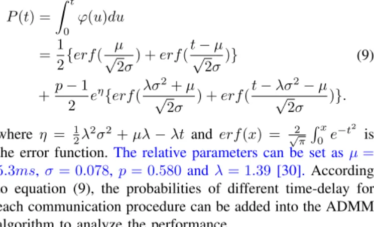
In order to calculate the time-delay probability of each communication for all nodes, the PDF (8) will be recalculated to derive the Cumulative Distribution Function (CDF) of time delay model as [20] P(t) = Z t 0 ϕ(u)du =1 2{erf( µ √ 2σ) +erf( t−µ √ 2σ)} +p−1 2 e η{erf(λσ√2+µ 2σ ) +erf( t−λσ2−µ √ 2σ )}. (9)
where η = 12λ2σ2+µλ−λt and erf(x) = √2
π
Rx
0 e −t2
is the error function.The relative parameters can be set asµ= 5.3ms,σ= 0.078,p= 0.580 andλ= 1.39[30].According to equation (9), the probabilities of different time-delay for each communication procedure can be added into the ADMM algorithm to analyze the performance.
Fig. 2: Illustration of timing diagram. (a) Synchronous algo-rithm; (b) Asynchronous algorithm.
Message transmission mechanism: The aim of this paper is to investigate the ADMM algorithm with stochastic time-delay. The detailed iterative process of ADMM algorithm with communication delay for kth iteration is summarized as follow: (Step 1) each individual augmented Lagrangian function Li(Xi) with linear constraints would be solved by
KKT conditions to achieve the new local variablesQi(k+ 1) andQ+i (k+ 1)independently;(Step 2) nodei transmits the new variable Qi(k+ 1) to node i−1. Meanwhile, node i would receive the newQi+1(k+ 1)from nodei+ 1; (Step 3) the new global variable Qi(k+ 1) and Lagrange multipliers
yi(k+ 1), y+i (k+ 1) can be obtained by (7b)-(7d); (Step 4)
nodeisends updated global variableQi(k+ 1)andVi(k+ 1)
to nodei+ 1. Nodeiwill simultaneously receive the updated variables from node i−1. Then the iterative process will be repeated until the result satisfies a certain error condition. The above communication mechanism shows that each node will exchange the information with backward and forward
neighbouring nodes independently in every iteration. It is easy to find that the mechanism has a synchronization issue. In this paper, both synchronous and asynchronous algorithms are proposed to analyze the performance of ADMM algorithm. The detail of both algorithms will be discussed below.
The synchronous distributed ADMM algorithm is outlined in Algorithm 1. We assume that the computation time tdm
(t1 tot2) and tdu (t3 tot4) are the constant time in Fig. 2. The red and pink lines are backward and forward links, which means each node only sends message to backward or forward neighbouring nodes. Fig. 2(a) is the synchronous algorithm timing diagram, where the maximum communication time is locked by the threshold time tds (assume t2 to t3 equals t4 to t5). According to equation (9), we set 6.3363 ms (10% probability of time-delay) as the tds. Each node will be
equipped with an external GPS to keep each step have the same clock. Specifically, after the step of calculation, only when communication time of backward or forward link reachestds,
each node will start the next step. It is a complete iteration period for the synchronous algorithm.
Algorithm 1: Synchronous ADMM Algorithm 1: process for local nodei,i∈1, ..., ν 2: initializelocal variablesXi(0), k=0.
3: repeat
4: update to obtainXi(k+ 1)
5: waittdm
6: transmitQi(k+ 1) to backward nodes 7: receive Qi+1(k+ 1)from forward nodes 8: waittds
9: update to obtainQi(k+ 1)
10: updateto obtainyi(k+ 1),yi+(k+ 1)
11: waittdu
12: transmitQi(k+ 1)to forward nodes
13: receiveQi−1(k+ 1) from backward nodes 14: waittds
15: k=k+1
16: untillsatisfied the defined minimum error 17: endprocess
An asynchronous algorithm is presented in Fig. 2(b). Each communication also has a bounded maximum transmission timetda, which is set to 9.6146 ms (0.1%delay probability). In
case of a delay, the message may lead the algorithm to remain in the status of receiving the message. This algorithm does not need to wait until all nodes have received the updated variables before beginning the next step. Every node can execute the update steps to obtain the new local variables independently and immediately when it receives the message. Hence, each node will not have idle status and more iterations can be obtained. However, the communication message comes from neighbouring nodes, it is possible that nodeihas not received any message from neighbouring nodes (perhaps the message is still in transit due to late transmission) when time reaches the tda. Then the previous data will be used to update the
variables in order to keep the algorithm running without extra waiting time. The outline of asynchronous algorithm is listed in Algorithm 2.
During the same time interval in Fig. 2, all nodes in
synchronous ADMM algorithm just finish one iterative period, but some nodes in asynchronous ADMM algorithm almost completes one and a half iterative period. It is obviously that asynchronous algorithm can shorten the iteration period and increase the number of iterations. Consequently, the asyn-chronous algorithm can speed up the convergence rate faster than the synchronous algorithm to obtain a high theoretical accuracy. We assume that all node can always receive the message within threshold time for no-delay case. If some nodes do not receive the message within threshold time, the message will be considered as lost. Then other measures will be taken to continue the next step.
Algorithm 2: Asynchronous ADMM Algorithm 1: processfor local nodei,i∈1, ..., ν
2: initializelocal variablesXi(0), k=0.
3: repeat
4: updateto obtainXi(k+ 1)
5: transmitQi(k+ 1)to backward nodes
6: receiveQi+1(k+ 1)from forward nodes 7: wait≤tda
8: updateto obtainQi(k+ 1)
9: updateto obtainyi(k+ 1),y+i (k+ 1)
10: transmitQi(k+ 1) to forward nodes
11: receiveQi−1(k+ 1)from backward nodes 12: wait≤tda
13: k=k+1
14: untillsatisfied the defined minimum error 15: end process
C. Convergence Analysis for Asynchronous ADMM Algorithm
The convergence analysis of synchronous ADMM algorithm has been investigated in [17], [19], [27]. In this section, the convergence behavior of asynchronous ADMM algorithm will be studied. Some assumptions regarding the problem are made. Let∇Fibe the gradient or subgradient ofFi in (3a). And we
also define kτ
i as a new sequence of node i, which implies
that the gradient calculation may use old parameters due to the delayed message or lost message.xiandxi are the global
and local variables for each node i, respectively. Then, the following assumptions are listed.
Assumption 1: For each node i, the individual function gra-dient∇Fi is Lipchitz continuous, and there exists a constant
Ki>0, such that
k ∇Fi(xi(k+ 1))− ∇Fi(xi(k+ 1))k
≤Kikxi(k+ 1)−xi(k+ 1)k
(10) In addition,X is a closed, convex and compact set. The power loss functionFi(xi)is bounded from below overX.
Assumption 2: The total delays are bounded. For each nodei, there exists finite constantTi such thatk−kτi ≤Ti for all k.
Assumption 3: For each nodei, the stepsizeρiis chosen large
αi=ρi− 2ρ+ 7Ki ρ2 i Ki(Ti+ 1)2−KiTi2>0 (11a) βi=ρi−7Ki>0 (11b)
Assumption 1 is the standard in the context of non-convex optimization [31] and is satisfied for most problems of interest. According to assumption 2, when xi is updated in
asyn-chronous algorithm, the parameter used to update the variables should be the latest received parameter. The convergence of the asynchronous algorithm can be verified by the following lemma.
Lemma 1: Suppose that assumptions 1, 2 and 3 hold true. Then we have the following true for asynchronous algorithm. (a) kyi(k+ 1)−yi(k)k22 ≤Ki2(Ti+ 1) Ti X κ=0 kx(k+ 1−κ)−x(k−κ)k2 2 (12)
(b) The augmented Lagrangian is lower bounded and satisfies
L({xi(k)};{xi(k)},{yi(k)}) ≥Plos− ν X i=1 Ki 2 diam 2(X)>−∞ (13)
The proof of Lemma 1 can be found in Appendix A. Lemma 1(a) presents that there exists certain finite k <∞ such that the augmented Lagrangian values are non-increasing after k iterations. Lemmas 1(b) presents that the Lagrangian is lower bounded. Then, we achieve that the augmented Lagrangian function is convergent.
The subsequent theorem proves the final convergence result and other properties.
Theorem 1: (a) The iterates generated by the asynchronous algorithm converges if the following is true
lim k→∞kxi(k+ 1)−xi(k)k= 0, i∈ν (14a) lim k→∞kxi(k+ 1)−xi(k)k= 0, i∈ν (14b) lim k→∞kyi(k+ 1)−yi(k)k= 0, i∈ν (14c)
(b) For each node i at k iterations, certain sequences
{{x∗i},{x∗i},{y∗i}}converges to the set of stationary solution
of (4.5) and satisfies
∇Fi(x∗i) +y
∗
i = 0, i∈ν (15a)
x∗i =x∗i, i∈ν (15b) The proof of Theorem 1 can be found in Appendix B. Note that it suffices to show that asynchronous algorithm converges to a stationary solution of (4) which is equivalent to (3). In other words, {x∗
i} can be the solution of (3). It is emphasized that
the asynchronous algorithm may not converge to a globally
optimal solution.
D. Delay-robust Strategies
The convergence performance for both algorithms will cer-tainly be affected when time-delay is considered, for example, unstable results, low quality results and slow convergence. Different measures will assess the effect of time-delay in both synchronous and asynchronous algorithms.
1) Strategy I-Skipping Strategy (SS): In this strategy, if the communication message is not delivered within the threshold time, the unreceived node will not carry out current step and skip it. Then this node will wait until the next successful com-munication. Other nodes will continue to update the variables by (7). The SS not only interrupts the normal update of the algorithm, but also affects the neighbouring nodes’ normal update of the algorithm due to the time-delay.
2) Strategy II-Previous Value Strategy (PVS): The PVS replaces the delayed message by using the saved data from the last successful communication. Each node can install a storage device to save the data generated from the previous normal iteration. When the delay occurs, the stored informa-tion can be invoked instead of the message that have not be received within the threshold time. The update of other nodes still follows equations (7). This strategy may decrease the convergence rate because the partial iterative processes using previous data can reduce the update of both self-node and neighbouring nodes. It is more suitable for certain scenarios that are prone to transmission delay while the requirement of optimization accuracy is not very stringent.
3) Strategy III-AR Strategy (ARS): The predicted value in advance is utilized instead of the previous saved message in the PVS. Forecast begins when the communication message is received in the last successful communication, which means no extra time is required. Suppose the relationship between past successfully received messages and current unreceived message can be estimated using previous saved data. TheAR model of orderω is defined as [32]
at=c+ ω X i=1 φiat−i+t =c+φ1at−1+φ2at−2+...+φωat−ω+t. (16)
whereω is the order of the AR model andφ1, ..., φω are the
AR coefficients which are constant, c is also the fixed value andtis the stochastic parameter that we define as white noise,
t ∼ T(0, σ2). In addition, a1, a2, ..., aT are the previous
values of time series data used to predict the current value. According to the AR coefficient, the likelihood function of the AR model can be written as
pl(φ, σ2) = T Y t=1 1 √ 2πσ2exp{− 1 2σ2(at− ω X i=1 φiat−i)2}. (17) where the parameters can be obtained by using the Yule-Walker method [33]. The performance of AR model is de-pended on the order. Decreasing the order against the time
se-ries data reduces the estimation performance of the AR model and increasing the order leads to more complex behavior which can even fail to obtain appropriate estimations. The Akaike-Information-Criterion(AIC) is adopted as the evaluation func-tion to balance the order and likelihood [34].
AIC=−2
T
X
t=1
ln{p(at|φ, σ2)}+ 2ω. (18)
whereωis the selected order of the AR model and the value of ωcan be chosen from the order index 1,2,3...,ω. The evaluation function of AIC will be applied to estimate the unreceived message. If the time-delay happens, the algorithm will adopt the predictive values to replace the unreceived variables. Other nodes will follow (6) to update the variables. For brevity, we have not included the detail of the AR derivation process.
4) Strategy VI-Weighted AR Strategy (WARS): The esti-mated value from AR strategy exists certain errors during the prediction process. Therefore, we propose to add a weighted term into the ADMM algorithm to reduce the error caused by the prediction to improve the convergence results. The ADMM recursive expression in (7) for kth iteration can be rewritten as Xiw(k+1) := arg min Xiw {Liw(Xiw) :H(Xiw)≤0, E(Xiw) = 0} (19a) Qiw(k+ 1) = 1 2(Q + iw(k+ 1) + (1 +γi)aiw+1(k)) + 1 ζi yiw+(k) (19b) yiw(k+ 1) =yiw(k) +ρ(Qiw(k+ 1)−(1 +γi)aiw−1(k)). (19c) where the iwis the set of nodes whose message do not arrive on time. γi and γi are the weighted factors. The weighted
terms γiaiw−1(k) and γiaiw+1(k) are added to execute the iterative steps if delay happens. Other nodes will continue to use the (6) to update the variables. The weighted factors can reduce the predictive error and optimize the predicted value to obtain a better convergence result.
E. Connection between WARS and Conventional ADMM
It is necessary to observe the difference to find the connec-tion between WARS and convenconnec-tional ADMM. Reference [27] presents the traditional ADMM iterative form for consensus minimization problem. Xi(k+ 1) := arg min Xi {Li(Xi) :H(Xi)≤0, E(Xi) = 0} (20a) Q(k+ 1) = 1 N N X i=1 (Qi(k+ 1) +1 ρyi(k)) (20b) yi(k+ 1) =yi(k) +ρ(Qi(k+ 1)−Q(k+ 1)). (20c)
Comparing (19) and (20), it is obviously that the traditional ADMM algorithm is a particular case of the WARS by setting Qi(k+ 1) =
Q+iw(k+1)+(1+γi)aiw+1(k)
2 , Qi(k+ 1) = (1 +γi)aiw−1(k) and 1ρ = ζ1i. All steps are set to use the
same coefficient 1ρ in the conventional ADMM. Contrarily, the WARS assigns the different coefficient ζ1
i instead of the constant coefficient 1ρ. In addition, the WARS adds different weighted terms γiaiw+1(k) and γiaiw−1(k) to each node because of the forecast error.
These changes can make the WARS to achieve a better efficiency than the traditional ADMM. To begin with, the traditional ADMM requires information exchange with all nodes to update the global variable Q(k+ 1). In contrast, the WARS is able to decrease the communication cost by communicating with limited neighbouring nodes. Furthermore, when delay happens, the unreceived message not only affects the variable update of self-node, but also affects the vari-able update of neighbouring nodes. Using modified predicted value in proposed WARS can decrease the error as much as possible against the traditional ADMM. In addition, the adopted weighted terms may produce a certain deviation from the original value which can improve the results from a local optimization to a global optimization. Finally, the conventional ADMM can only optimize its convergence speed by adjusting the penalty factor ρ, since other parameters are fixed. Whereas, the WARS has the flexibility by adjusting both weighted termsγiaiw+1(k), γiaiw−1(k) and coefficient term
1
ζi. Consequently, the WARS not only has the potential to reduce the volatility, but also accelerate the convergence speed to obtain a better optimization result.
IV. SIMULATION RESULTS
In order to verify the ADMM algorithm with communi-cation delay, a 33-bus medium-voltage DN has been used as a case study [35]. It contains 33 buses and 32 branches. In addition, four wind DGs (2,12,15,18) and four solar DGs (23,25,27,33) are installed in the network [36].
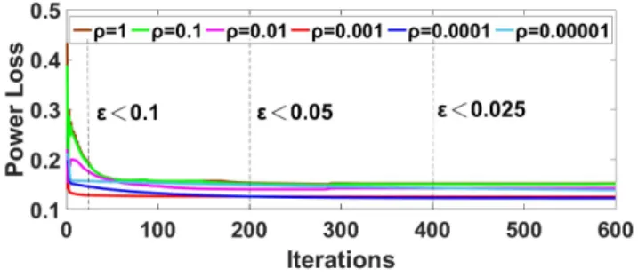
Fig. 3: Illustration of convergence speed of distribution ADMM algorithm with different values of penalty factor ρ.
A. Observation of General Convergence Speed
To maximize the convergence speed, the applied ADMM formula has two important parameters, the penalty factorρand the convergence toleranceε. Fig. 3 illustrates the convergence speed of synchronous ADMM with different ρ, which is decreased from 1 to 0.00001. The high values of ρtypically have a slow convergence speed and poor iterative results. The best choice ofρwhich provide the fastest convergence speed is
0.001 in the early stage of the iteration process. Subsequently, the convergence speed forρ= 0.001is slower than the speed for ρ= 0.0001 after 200 iterations. In other different cases, a little higher or smaller value of ρmay result in a slightly better convergence speed.
Fig. 3 also shows the different tolerance values for different iterations. The ADMM only needs 9 iterations to reach the tolerance goal of less than 10%compared to centralized result. However, the error is only less than 5% after 200 iterations and 2.5% after 400 iterations. It is typically that the ADMM algorithm has a faster convergence rate at the beginning of the iteration process. In some special cases, it also should be noted that setting a high tolerance value (e.g., ε= 0.1 ) may results in a large fluctuation. In this paper, we set the tolerance value asε <0.05which could also help to choose the penalty factorρ= 0.001with faster convergence rate.
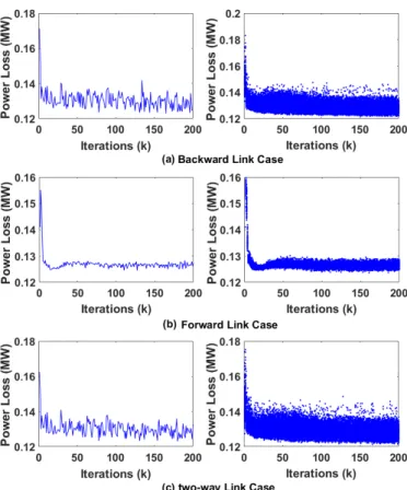
Fig. 4: Comparison of convergence speed and statistic results of three different cases for synchronous SS (1000 runs each).
Fig. 5: (a) Comparison of different synchronous strategies, (b) Comparison of synchronous ARS and WARS (100 runs each).
B. Performance of Synchronous algorithm
In this section, the communication delay is applied to synchronous algorithm to test the performance. We divide communication into three different cases, the backward link case, the forward link case and two-way link case. Fig. 4 shows the effect of convergence speed in synchronous SS. The left side of Fig. 4 presents the fluctuated convergence results in three cases under a fixed probability of time-delay. For these three cases, the optimization results always have a larger fluctuation during the iterations. The result in forward link has less fluctuation range than that in backward link. Meanwhile, two-way link case has the largest fluctuation. The right side of Fig. 4 demonstrates the statistical results for these three cases (1000 stochastic time-delay runs for each case). The maximum fluctuation range is 21.33% in backward link case, 11.17% in forward link and 22.58% in two-way link. Overall the results indicate that the fluctuation mainly depends on the communication of step 2 in Fig. 2(a), which means the global reactive power variableQi(k+ 1)would significantly
influence the minimization results for both self-node and other neighbour nodes in (5).
Fig. 5(a) shows the optimization results of different syn-chronous strategies under a fixed time-delay scenario. Only two-way link case is performed as the space limitation. It is clear that the results of PVS dramatically reduce the fluctuation range compared to the results of SS. However, the optimization result after 200 iterations does not converge to a desirable value (near 0.13 MW) and the maximum 8.98% error could be very inefficient. The warm-starting of ADMM algorithm (forecast in advance) can be utilized to improve both the fluctuation in SS and the convergence speed in PVS. In Table I, 1000 stochastic time-delay runs are simulated for each strat-egy. The smaller variance values indicate the less fluctuation. Table I shows that the synchronous ARS obtains a better result against the PVS. Although the proposed ARS speed up the convergence rate, the result still has a fluctuation because of the forecasting error. Hence, weighted terms are added to improve the estimation error to optimize the results. The peculiarity of WARS shows an increased convergence speed, decreased fluctuation range and even better optimization result than that in the synchronous no-delay case. Comparing with the results 0.1258 MW of synchronous no-delay case, the mean value of WARS can converge to 0.1243 MW which dramatically improve the result. The results in synchronous WARS demonstrate that it is an efficient strategy from a synchronous distributed optimization perspective.
Fig. 6: (a) Comparison of different asynchronous strategies, (b) Enlarged version from 400 ms to 1200 ms.
TABLE I: Statistical Results with 1000 Runs for Each Strategy
Synchronous Asynchronous
SS PVS ARS WARS SS PVS ARS WARS
M ean 0.1287 0.1298 0.1283 0.1243 0.1239 0.1238 0.1237 0.1227
V ariance 1.16E−5 7.12E−7 3.16E−7 6.20E−8 6.96E−7 2.16E−7 1.15E−7 1.73E−7
C. Performance of Asynchronous Algorithm
Fig. 6(a) demonstrates the results of the different asyn-chronous strategies. The result is based on the wall clock time because the asynchronous algorithm do not require a synchro-nization device to wait in the process. Although the asyn-chronous strategy has a larger threshold time tolerance, the result in asynchronous no-delay case has a better optimization result which can achieve 0.1238 MW compared to the 0.1258 MW in synchronous no-delay case at the same time interval. Furthermore, the synchronous strategy requires 1260 ms to achieve 0.1258 MW, but the asynchronous strategy reaches the same result only after 300 ms. The increased convergence speed by the asynchronous algorithm mainly comes from the reduction of the waiting time and the increasing number of the iterations.
Meanwhile, the result of asynchronous SS show that the time-delay still brings a slight influence on the stability of the convergence result with 0.1%delay probability. The mean value of asynchronous WARS in Table I presents that the result can be improved to 0.1227 MW. Furthermore, the fluctuation performance is also improved with such low probability of delay. Consequently, the proposed WARS can significantly improve the optimization results from an asynchronous op-timization perspective.
Fig. 7: The convergence results for loss communication case.
D. Performance of Loss communication
The above simulation is based on the practical commu-nication system which is low probability of commucommu-nication delay. However, in case some nodes’ communication devices are out of work, the normal convergence rate will have large fluctuation even if the probability of communication delay is low. The simulation results in Fig. 7 show the convergence results of different strategies both in synchronous and asyn-chronous algorithms. In this case, we assume that these nodes (node 15, 18, 23, 25) are out of work. Fig. 7(a) presents that the proposed WARS can effectively reduce the fluctuation of
TABLE II: Statistical results with 1000 runs for each strategies of loss communication case
Mean Variance Syn-Skipping Strategy 0.1289 7.11E-6
Syn-Previous Value Strategy 0.1308 2.30E-5
Syn-AR Strategy 0.1299 1.53E-5
Syn-Weighted AR Strategy 0.1260 8.85E-6
Asyn-Skipping Strategy 0.1237 5.52E-6
Asyn-Previous Value Strategy 0.1250 1.02E-7
Asyn-AR Strategy 0.1231 5.16E-7
Asyn-Weighted AR Strategy 0.1230 6.62E-7
experimental results. In addition, the statistical results in Table II show that the mean value can be reduce to 0.1260 MW and the variance value is the smallest among the synchronous strategies. Comparing with the synchronous algorithm, the asynchronous algorithms can not only improve the mean value from 0.1260 MW to 0.1230 MW, but also demonstrate the lowest fluctuation of experimental results in Fig. 7(b) and Table II.
V. CONCLUSION
The future smart grid system will become more and more granular because of the increased penetration of renewable generators, distributed storage and electric vehicles. The in-vestigation of a distributed ADMM algorithm considered communication delay model was discussed in this paper. Both synchronous and asynchronous algorithms combined with stochastic delay analyzed the convergence results compared to the no-delay algorithm. It shows that time-delay would signifi-cantly affect the performance of results in both algorithms. The simulations presented that the proposed WARS can effectively improve the volatility and achieve a better optimization result compared to other strategies.
It should be noted that this paper is a first step to developing the communication model into the distributed problem in power system. Developing a more accurate communication model, proposing a more effective strategy and investigating the cyber-attack would be very meaningful for future work.
APPENDIXA
Proof of Lemma 1(a): According to the update of global variables (20), we can obtain that the following is true
∇Fi(xi(kiτ+ 1)) +yi(k) +ρi(xi(k+ 1)−xi(k+ 1)) = 0,
(21) Further, from (21), we have
∇Fi(xi(kiτ+ 1)) =−yi(k+ 1), (22)
Similarly, it also have the following equality for iterationk
∇Fi(xi(kiτ)) =−yi(k), (23)
Therefore, when the new information is delayed or lost for each nodei, it follows that
∇Fi(xi(kiτ+ 1)) =∇Fi(xi(kiτ)), (24)
According to (24), we have
kyi(k+ 1)−yi(k)k22= 0, (25) It means that Lemma 1(a) is true when message delayed or loss occurred. If the information arrives, we also have the following results by using triangle inequality.
kyi(k+ 1)−yi(k)k22 =k ∇Fi(xi(kiτ+ 1))− ∇Fi(xi(kτi))k 2 2 ≤Ki2kxi(kiτ+ 1)−xi(kτi)k ≤Ki2( Ti X κ=0 kxi(k+ 1−κ)−xi(k−κ)k)2 ≤Ki2(Ti+ 1) Ti X κ=0 kxi(k+ 1−κ)−xi(k−κ)k22. (26)
Subsequently, the desired result in Lemma 1(a) is achieved.
Proof of Lemma 1(b): According to the Lipschitz continuity of ∇Fi and triangle inequality, which implies that
Fi(xi(k+ 1)) ≤Fi(xi(k+ 1)) +∇Fi(xi(k+ 1))kxi(k+ 1)−xi(k+ 1)k +Ki 2 kxi(k+ 1)−xi(k+ 1)k 2 2 =Fi(xi(k+ 1))− k ∇Fi(xi(k+ 1))− ∇Fi(xi(k+ 1))k kxi(k+ 1)−xi(k+ 1)k+∇Fi(xi(k+ 1)) kxi(k+ 1)−xi(k+ 1)k+ Ki 2 kxi(k+ 1)−xi(k+ 1)k 2 2 ≤Fi(xi(k+ 1)) +∇Fi(xi(k+ 1))kxi(k+ 1)−xi(k+ 1)k +3Ki 2 kxi(k+ 1)−xi(k+ 1)k 2 2. (27) Further, from (22), we have
L({xi(k)};{xi(k)},{yi(k)}) = ν X i=1 (Fi(xi(k+ 1)) +yi(k+ 1)kxi(k+ 1) −xi(k+ 1)k+ ρi 2 kxi(k+ 1)−xi(k+ 1)k 2 2) ≥ ν X i=1 (Fi(xi(k+ 1)) + ρi−3Ki 2 kxi(k+ 1) −xi(k+ 1)k22+k ∇Fi(xi(k+ 1)) − ∇Fi(xi(kτi + 1))kkxi(k+ 1)−xi(k+ 1)k). (28)
According to the Cauchy-Schwarz inequality on the last term in (27), it follows that
L({xi(k+ 1)};{xi(k+ 1)},{yi(k+ 1)}) ≥Plos+ ρi−3Ki 2 X kxi(k+ 1)−xi(k+ 1)k22 − k ∇Fi(xi(k+ 1))− ∇Fi(xi(kτi + 1))kkxi(k+ 1) −xi(k+ 1)k ≥Plos+ ρi−4Ki 2 X kxi(k+ 1)−xi(k+ 1)k22 −Ki 2 kxi(k+ 1)−xi(k τ i + 1)k22 ≥Plos− ν X i=1 Ki 2 diam 2(X)>−∞. (29)
where the last inequality follows the fact that X is compact in assumption 1 and ρi−7Ki>0in assumption 3
APPENDIXB
Proof of Theorem 1(a): According to Lemma 1, it is true that L({xi(k)};{xi(k)},{yi(k)}) converges ask→ ∞.
Therefore, it holds from Lemma 1(a) that
lim
k→∞kxi(k+ 1)−xi(k)k→0, i∈ν (30a)
lim
k→∞kxi(k+ 1)−xi(k)k→0, i∈ν (30b) Then, using (30) into (26), it follows that
lim
k→∞kyi(k+ 1)−yi(k)k→0, i∈ν (31a)
lim
k→∞kxi(k)−xi(k)k→0, i∈ν (31b) Proof of Theorem 1(b): According to (31), it is true that certain sequences{{x∗i},{x∗i},{y∗i}}exist which follows that
∇Fi(x∗i) +y
∗
i = 0, i∈ν (32a)
x∗i =x∗i, i∈ν (32b) Since xi(k+ 1)∈ X, it holds that x∗i ∈ X. Once we can
present that the primal feasibility gap goes to zero, the proof for stationary solution is straightforward, which proves (15). The related reference can be found in [37].
REFERENCES
[1] N. D. Hatziargyriou and A. P. S. Meliopoulos, “Distributed energy sources: technical challenges,”2002 IEEE Power Engineering Society Winter Meeting. Conference Proceedings (Cat. No.02CH37309), vol. 2, pp. 1017–1022, 2002.
[2] F. Katiraei and M. R. Iravani, “Power management strategies for a microgrid with multiple distributed generation units,”IEEE Transactions on Power Systems, vol. 21, no. 4, pp. 1821–1831, Nov 2006. [3] D. K. Molzahn, F. Drfler, H. Sandberg, S. H. Low, S. Chakrabarti,
R. Baldick, and J. Lavaei, “A survey of distributed optimization and control algorithms for electric power systems,”IEEE Transactions on Smart Grid, vol. 8, no. 6, pp. 2941–2962, Nov 2017.
[4] J. Peschon, D. S. Piercy, W. F. Tinney, O. J. Tveit, and M. Cuenod, “Optimum control of reactive power flow,”IEEE Transactions on Power Apparatus and Systems, vol. PAS-87, no. 1, pp. 40–48, Jan 1968. [5] J. F. Dopazo, O. A. Klitin, G. W. Stagg, and M. Watson, “An
optimiza-tion technique for real and reactive power allocaoptimiza-tion,”Proceedings of the IEEE, vol. 55, no. 11, pp. 1877–1885, Nov 1967.
[6] S. Granville, “Optimal reactive dispatch through interior point methods,” IEEE Transactions on Power Systems, vol. 9, no. 1, pp. 136–146, Feb 1994.
[7] B. Zhao, C. X. Guo, and Y. J. Cao, “A multiagent-based particle swarm optimization approach for optimal reactive power dispatch,”IEEE Transactions on Power Systems, vol. 20, no. 2, pp. 1070–1078, May 2005.
[8] N. Takahashi and Y. Hayashi, “Centralized voltage control method using plural D-STATCOM with controllable dead band in distribution system with renewable energy,”Proc. 2012 3rd IEEE PES International Conference and Exhibition on Innovative Smart Grid Technologies (ISGT Europe), pp. 1–5, Oct 2012.
[9] C. Dwork, N. Lynch, and L. Stockmeyer, “Consensus in the presence of partial synchrony,”J. ACM, vol. 35, no. 2, pp. 288–323, Feb 1988. [10] R. Baldick, B. H. Kim, C. Chase, and Y. Luo, “A fast distributed
implementation of optimal power flow,”IEEE Transactions on Power Systems, vol. 14, no. 3, pp. 858–864, Aug 1999.
[11] E. Dall’Anese, H. Zhu, and G. B. Giannakis, “Distributed optimal power flow for smart microgrids,”IEEE Transactions on Smart Grid, vol. 4, no. 3, pp. 1464–1475, Sep 2013.
[12] A. Y. S. Lam, B. Zhang, and D. N. Tse, “Distributed algorithms for optimal power flow problem,” 2012 IEEE 51st IEEE Conference on Decision and Control (CDC), pp. 430–437, Dec 2012.
[13] Y. Wang, L. Wu, and S. Wang, “A fully-decentralized consensus-based admm approach for dc-opf with demand response,”IEEE Transactions on Smart Grid, vol. 8, no. 6, pp. 2637–2647, Nov 2017.
[14] V. Calderaro, G. Conio, V. Galdi, G. Massa, and A. Piccolo, “Optimal decentralized voltage control for distribution systems with inverter-based distributed generators,”IEEE Transactions on Power Systems, vol. 29, no. 1, pp. 230–241, Jan 2014.
[15] L. Y. Tseng and S. B. Yang, “A genetic approach to the automatic clustering problem,”Pattern Recognition, vol. 34, no. 2, pp. 415 – 424, 2001.
[16] P. Łulc, S. Backhaus, and M. Chertkov, “Optimal distributed control of reactive power via the alternating direction method of multipliers,”IEEE Transactions on Energy Conversion, vol. 29, no. 4, pp. 968–977, Dec 2014.
[17] Q. Ling, Y. Liu, W. Shi, and Z. Tian, “Weighted admm for fast decen-tralized network optimization,”IEEE Transactions on Signal Processing, vol. 64, no. 22, pp. 5930–5942, Nov 2016.
[18] A. Abboud, R. Couillet, M. Debbah, and H. Siguerdidjane, “Asyn-chronous alternating direction method of multipliers applied to the direct-current optimal power flow problem,” in2014 IEEE International Conference on Acoustics, Speech and Signal Processing (ICASSP), May 2014, pp. 7764–7768.
[19] Y. Zhang, E. Dall’Anese, M. Hong, S. Dhople, and Z. Xu, “Regulation of renewable energy sources to optimal power flow solutions using admm,” 2017 American Control Conference (ACC), pp. 3394–3399, May 2017. [20] J. Zhang, S. Nabavi, A. Chakrabortty, and Y. Xin, “Admm optimization strategies for wide-area oscillation monitoring in power systems under asynchronous communication delays,” IEEE Transactions on Smart Grid, vol. 7, no. 4, pp. 2123–2133, Jul 2016.
[21] R. Zhang and J. T. Kwok, “Asynchronous distributed admm for consen-sus optimization,”Proceedings of the 31 st International Conference on Machine Learning, pp. 1701–1709, 2014.
[22] T. H. Chang, M. Hong, W. C. Liao, and X. Wang, “Asynchronous distributed admm for large-scale optimization part i: Algorithm and
convergence analysis,”IEEE Transactions on Signal Processing, vol. 64, no. 12, pp. 3118–3130, Jun 2016.
[23] M. Baran and F. F. Wu, “Optimal sizing of capacitors placed on a radial distribution system,”IEEE Transactions on Power Delivery, vol. 4, no. 1, pp. 735–743, Jan 1989.
[24] N. R. Ullah, K. Bhattacharya, and T. Thiringer, “Wind farms as reactive power ancillary service providers-technical and economic issues,”IEEE Transactions on Energy Conversion, vol. 24, no. 3, pp. 661–672, Sep 2009.
[25] S. Kundu and I. A. Hiskens, “Distributed control of reactive power from photovoltaic inverters,” in 2013 IEEE International Symposium on Circuits and Systems (ISCAS2013), May 2013, pp. 249–252. [26] K. Turitsyn, P. Sulc, S. Backhaus, and M. Chertkov, “Local control of
reactive power by distributed photovoltaic generators,” in 2010 First IEEE International Conference on Smart Grid Communications, Oct 2010, pp. 79–84.
[27] S. Boyd, N. Parikh, E. Chu, B. Peleato, and J. Eckstein, “Distributed optimization and statistical learning via the alternating direction method of multipliers,” Foundations Trends Mach. Learn., vol. 3, no. 1, pp. 1–122, 2011.
[28] S. Boyd and L. Vandenberghe, Convex Optimization. Cambridge University Press, Mar 2004.
[29] C. J. Bovy, H. T. Mertodimedjo, G. Hooghiemstra, H. Uijterwaal, and P. V. Mieghem, “Analysis of end-to-end delay measurements in internet,” submitted to PAM, 2002.
[30] G. Hooghiemstra and P. V. Mieghem, “Delay distributions on fixed inter-net paths,”Dept. Inf. Technol. Syst., Delft Univ., Delft, The Netherlands, Tech. Rep. 20-011-020, 2001.
[31] S. Magnsson, P. C. Weeraddana, M. G. Rabbat, and C. Fischione, “On the convergence of alternating direction lagrangian methods for nonconvex structured optimization problems,” IEEE Transactions on Control of Network Systems, vol. 3, no. 3, pp. 296–309, Sep 2016. [32] G. Hendrantoro, A. Mauludiyanto, and P. Handayani, “An autoregressive
model for simulation of time-varying rain rate,”2004 10th International Symposium on Antenna Technology and Applied Electromagnetics and URSI Conference, pp. 1–4, Jul 2004.
[33] M. G. Anderson, N. Zhou, J. W. Pierre, and R. W. Wies, “Bootstrap-based confidence interval estimates for electromechanical modes from multiple output analysis of measured ambient data,”IEEE Transactions on Power Systems, vol. 20, no. 2, pp. 943–950, May 2005.
[34] H. Akaike, “Information theory and an extension of the maximum likeli-hood principle,”Springer Series in Statistics, Perspectives in Statistics., vol. 1, pp. 610–624, 1992.
[35] M. Baran and F. Wu, “Network reconfiguration in distribution systems for loss reduction and load balancing,” IEEE Transactions on Power Delivery, vol. 4, no. 2, pp. 1401–1407, Apr 1989.
[36] J. Xu, H. Sun, and C. Dent, “The coordinated voltage control meets imperfect communication system,” 2016 IEEE PES Innovative Smart Grid Technologies Conference Europe (ISGT-Europe), pp. 1–5, Oct 2016.
[37] M. Hong, Z. Luo, and M. Razaviyayn, “Convergence analysis of alternating direction method of multipliers for a family of nonconvex problems,”SIAM Journal On Optimization, vol. 26, no. 1, pp. 337–364, 2016.