On the implementation of a log-barrier progressive hedging method for multistage stochastic programs

(1)

Contents lists available atScienceDirect

Journal of Computational and Applied

Mathematics

journal homepage:www.elsevier.com/locate/cam

On the implementation of a log-barrier progressive hedging method for

multistage stochastic programs

I

Xinwei Liu

a,∗

, Kim-Chuan Toh

b

, Gongyun Zhao

b

a_{Department of Applied Mathematics, Hebei University of Technology, Beichen Campus, Tianjin 300401, China} b_{Department of Mathematics, National University of Singapore, 2 Science Drive 2, Singapore 117543, Singapore}

a r t i c l e i n f o

Article history:

Received 15 April 2007

Received in revised form 30 December 2009

Keywords:

Progressive hedging method Multistage stochastic programs Lagrangian dual

Log-barrier method

a b s t r a c t

A progressive hedging method incorporated with self-concordant barrier for solving multistage stochastic programs is proposed recently by Zhao [G. Zhao, A Lagrangian dual method with self-concordant barrier for multistage stochastic convex nonlinear programming, Math. Program. 102 (2005) 1–24]. The method relaxes the nonanticipativity constraints by the Lagrangian dual approach and smoothes the Lagrangian dual function by self-concordant barrier functions. The convergence and polynomial-time complexity of the method have been established. Although the analysis is done on stochastic convex programming, the method can be applied to the nonconvex situation. We discuss some details on the implementation of this method in this paper, including when to terminate the solution of unconstrained subproblems with special structure and how to perform a line search procedure for a new dual estimate effectively. In particular, the method is used to solve some multistage stochastic nonlinear test problems. The collection of test problems also contains two practical examples from the literature. We report the results of our preliminary numerical experiments. As a comparison, we also solve all test problems by the well-known progressive hedging method.

1. Introduction

We consider the following stochastic program with recourse:

min q0

(

x

)

+

Eξ1Q1

(

x

, ξ

1

),

(1.1)

s.t. x

∈

X

,

where, fort

=

1

,

2

, . . . ,

T, the recourse functions are recursively defined by

Qt

(

x

,

y1

, . . . ,

yt−1

,

ξ

ˆ

1

, . . . ,

ξ

ˆ

t

)

=

min yt

qt

(

x

,

y1

, . . . ,

yt−1

,

yt

,

ξ

ˆ

1

, . . . ,

ξ

ˆ

t

)

+

E_ξ_t₊₁Qt+1

(

x

,

y1

, . . . ,

yt

,

ξ

ˆ

1

, . . . ,

ξ

ˆ

t

, ξ

t+1

)

|

(

x

,

y1

, . . . ,

yt

)

∈

Y_ξˆ₁_,...,_ξˆ_t

,

(1.2) QT+1

=

0

.

(1.3)

I _{Research is partially supported by NUS Academic Research Grant R-146-000-006-112, Grants 10571039 and 10971047 of National Natural Science} Foundation of China.

∗_{Corresponding author.}

(2)

Here

ξ

ˆ

iis a realization of the random vector

ξ

i;yi

∈ <

niis the decision vector in theith stage, which is generated recursively

by(1.2), and it depends onx

,

y1

, . . . ,

yi−1and

ξ

ˆ

1

, . . . ,

ξ

ˆ

i(hence is random);qt,t

=

0

,

1

, . . . ,

T, are real-valued functions on

<

nt_{. For}_t

_≥

_1,_q

tis random since it is related to

ξ

ˆ

1

, . . . ,

ξ

ˆ

t. The setsXandY_ξˆ₁_,...,_ξˆ_tare assumed to be convex. AgainY_ξˆ₁_,...,_ξˆ_t

depends on random variables. The details on the formulation of multistage stochastic programs can be found, for example, in [1,2].

There are many works devoted to stochastic linear programs, especially to two-stage stochastic linear programs,

see [3,4,1,5–10], and references therein. Extending these methods to solving multistage stochastic nonlinear programming is

not straightforward, since they used the special structures and properties of stochastic linear programs, and each additional stage can incur enormous complexity.

Scenario analysis technique was introduced to deal with multistage stochastic programs in [11], where the authors

considered stochastic programs with a finite number of scenarios and each scenario occurred with a fixed and known probability.

Berland and Haugen [12] presented a different way of defining scenarios and hence for the same problem the number of

scenarios and the size for each scenario may not be the same. They showed that the scenario analysis technique is flexible and can be used for different kinds of problems.

Based on a scenario aggregation technique, Rockafellar and Wets [11] proposed the progressive hedging method, which

is an iterative algorithm for multistage stochastic programming. This method associates with each scenariosa vector of

variableszs

=

(

xs

;

ys₁

;

. . .

;

ys_T

)

, so that the original problem can be decomposed into a collection of smaller subproblems,

each associated with a scenario. Then the method progressively hedgesxs_{(as well as}_ys

1

, . . . ,

ysT−1) so that eventuallyxs

=

x

holds for alls. The technique for realizing this idea mathematically is to impose a set of constraints, including e.g.xs

=

xs+1

(the so-called nonanticipativity constraints), and then to relax these constraints by using the Lagrangian dual. Suppose

that there are a finite number of realizations of the random vector

ξ

=

(ξ

₁

, ξ

₂

, . . . , ξ

_T

)

(sampling can be introduced if

ξ

has infinitely many realizations, and a realization is also called a scenario). LetSbe the total number of scenarios, and

ps

₍

_s

₌

₁

_{, . . . ,}

_S

₎

_{is the probability associated with the}_s_{th scenario. Suppose that the dimensions of}_x_,_y

1

, . . . ,

yT are

n0

,

n1

, . . . ,

nT, respectively. Let

n

=

n0

+

n1

+ · · · +

nT

.

(1.4)

The problem(1.1)–(1.3)can be reformulated as follows:

min F

(

z

)

:=

S

X

s=1 psfs

(

zs

)

(1.5) s.t. zs

∈

Xs

⊂ <

n

,

s

=

1

, . . . ,

S (1.6) z

=

(

z1

;

z2

;

. . .

;

zS

)

∈

Z

⊂ <

nS (1.7)

wherezs

:=

(

xs

;

ys₁

;

. . .

;

y_Ts

)

∈ <

nconsists of the decision vectors in all the stagest

=

0

,

1

, . . . ,

T,Xsis a feasible set

(assumed to be convex),fs

_{: <}

n

_{→ <}

_{is defined by}_fs

₍

_zs

₎

₌

_q

0

(

xs

)

+

q1

(

xs

,

ys1

;

ξ

1s

)

+ · · · +

qT

(

xs

,

ys1

, . . . ,

ysT

;

ξ

1s

, . . . , ξ

Ts

)

for thesth scenario

(ξ

₁s

, . . . , ξ

_Ts

)

,Zis a linear subspace of

<

nS _and_z

_∈

_Z_if_zs1,`

₌

_zs2,`_whenever

ξ

s1

`

=

ξ

`s2 for all

`

≤

t (wherezs,`is the

`

th subvector ofzs,zs,0

=

xsandzs,t

=

ys_tfort

=

1

, . . . ,

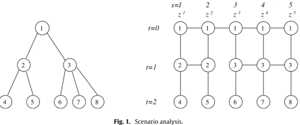
T). InFig. 1, we give an illustration on how the

subspaceZis constructed. The decision vectorsz1

_{, . . . ,}

_z5_{share the same history at stage}_t

₌

_{0, and thus we must ensure}

thatz1,0

=

z2,0

=

z3,0

=

z4,0

=

z5,0. Indeed,zs,0

=

xs

=

xfor alls

=

1

, . . . ,

5. Similarly,z1

,

z2share the same history at t

=

1, and thus we must havez1,1

₌

_z2,1_{. For}_z3

_,

_z4

_,

_z5_{at stage}_t

₌

_{1, we must have}_z3,1

₌

_z4,1

₌

_z5,1_{. In matrix form, we} have the following constraint forz

=

(

z1

_;

_{. . .}

_;

_z5

₎

_:







I

−I

I

−I

I

−I

I

−I

I

−I

I

−I

I

−I













z1,0 z2,0 z3,0 z4,0 z5,0 z1,1 z2,1 z3,1 z4,1 z5,1







=

0

,

(1.8)

whereIdenotes the identity matrix of appropriate dimension. Thus,z

∈

Zif and only ifzis a solution of(1.8).

The constraint in(1.7),z

∈

Z, is the nonanticipativity constraint. The representation of the subspaceZis not unique. In

general we writez

∈

ZasAz

=

0, whereAis a matrix. The Lagrangian dual relaxing the constraint(1.7)is expressed as

max

(3)

Fig. 1. Scenario analysis.

where thedual objective functionΘ

(

u

)

is given by

Θ

(

u

)

:=

min

F

(

z

)

−

uTAz

|

z

=

(

z1

;

. . .

;

zS

)

∈

X1

× · · · ×

XS

.

(1.10)

As u tends to the optimal dual solution, the corresponding optimal solution z of (1.10) will tend to satisfying the

nonanticipativity constraintAz

=

0, and hence will tend to the optimal solution of the original problem(1.5)–(1.7).

An apparent disadvantage of using program(1.9)is that the dimension of the dual vectoruis approximately the same

as that of the original problem(1.1)–(1.3). However, since the structure of the matrixAis simple (see the example in(1.8)),

algorithms based on problem(1.9)–(1.10)are much easier to program and more efficient to implement than algorithms

based on the original problem(1.1)–(1.3).

It is known that the augmented Lagrangian method is more efficient than the Lagrangian dual method generally.

Rockafellar and Wets [11] used the augmented Lagrangian method instead of(1.10). That is,

Θ

(

u

)

:=

min

F

(

z

)

−

uTAz

+

1 2

β

kAzk

2

_|

_z

₌

₍

_z1

_;

_{. . .}

_;

_zS

₎

_∈

_X1

_{× · · · ×}

_XS

.

(1.11)

They still call it the progressive hedging method (PHM in short).

Mulvey and Vladimirou [13] applied the progressive hedging method to stochastic generalized networks and achieved

satisfactory results. Based on their numerical experiences for the solution of stochastic fisheries management models by

PHM, Helgason and Wallace [14] suggested to solve the scenario subproblems in each iteration approximately. It has

been noted in [13–15] that the numerical behaviour of PHM can be affected significantly by the selection of the penalty

parameter

β

associated with the proximal term. The convergence of PHM can be very slow if this parameter is not selected

appropriately.

Based on scenario analysis and representation of multistage stochastic programs as a tree-like form, Ruszczyński [16]

proposed a new parallel decomposition method, with which all subproblems can be solved in parallel and information can be exchanged asynchronously. Computational experiments show that with a moderate number of processors, it can

obtain substantial gains in efficiency for large problems. Ruszczyński [17] considered solving a class of convex optimization

problems with the formulation(1.5)–(1.7). A decomposition method based on a separable approximation of the augmented

Lagrangian function was analyzed. It was shown that the convergence properties of the method were dependent on the

sparsity of the coefficient matrix for the constraint(1.7). Liu and Fukushima [18], Liu and Zhao [19] also considered the

scenario formulation of multistage stochastic programs, where [18] noticed that the coefficient matrix may not be of full

rank in the formulation and preprocessing is often necessary in developing rapid decomposition methods, [19] presented a

decomposition method based on SQP for solving a class of multistage stochastic nonlinear programs with nonlinear equality constraints.

A new iterative method based on progressive hedging was proposed recently in [20], who relaxes the nonanticipativity

constraints by the Lagrangian dual approach and smooths the Lagrangian dual function by self-concordant barrier functions

so that higher-order methods such as Newton’s method can be applied. In [20] this method was referred to as barrier

Lagrangian dual method. Because ‘‘progressive hedging’’ more aptly describes its nature, we will call the method proposed in [20] asbarrier progressive hedging method, in short BPHM, and the method proposed in [11] aspenalty progressive hedging method, in short PPHM. Zhao [20] focused on fundamental theoretical aspects of the method, such as global convergence and polynomial-time complexity.

In this paper, we will describe the implementation on the BPHM method in detail. An algorithm based on this method is applied to solve some multistage stochastic nonconvex nonlinear programming problems. The results are compared with those obtained by PPHM.

In spite of their importance, stochastic nonlinear programs have been relatively understudied. There still does not exist any standard collection of test problems for stochastic nonlinear programs in the literature. We construct the test problems here by adding some nonlinear terms to the objective and adding some nonlinear constraints in the set of constraints of the stochastic linear programs with coefficients generated by random number generators. Two practical examples from the

(4)

literature are also described and solved by the algorithms. We admit that the considered test problems are very small and not enough to demonstrate the efficiency of the BPHM method. Nevertheless, we hope that our attempts and discussions here could be helpful in providing some potential clues of the method in solving larger scale stochastic nonlinear programs. Certainly, systematic tests must be carried out when a collection of benchmark test problems is available.

This paper is organized as follows. In Section2, PPHM is described. We state BPHM and discuss some issues on its

implementation in Section3. Some multistage stochastic programming problems and the corresponding numerical results

are presented in Section4.

2. The penalty progressive hedging method

In this section we briefly describe the progressive hedging method proposed in [11]. Here we call it the penalty

progressive hedging method to distinguish it from the method in the next section.

Suppose thatKt _{is a set of scenarios with the same history up to stage}_t_,_pi_{is the probability associated with the}_i_th

scenario. Rockafellar and Wets [11] wrote the nonanticipativity constraints as

zi,t

=

_P

1 k∈Kt pk

X

j∈Kt pjzj,t

,

i

∈

Kt

,

t

=

0

,

1

, . . . ,

T

,

(2.1)

wherezi,t_{is the subvector associated with stage}_t_{. In particular, if all}_pj

₍

_j

₌

₁

_{, . . . ,}

_S

₎

_{are the same, i.e.}_pj

₌

1

S for allj, then (2.1)reduces to the simple situation:

zi,t

=

1

|

Kt

_|

X

j∈Kt

zj,t

,

i

∈

Kt

,

(2.2)

where

|

Kt

_|

_{is the cardinality of}_Kt_.

For simplicity, we consider only the simple case(2.2)in this paper. Then the nonanticipativity constraintz

∈

Zof the

form(2.2)can be written as Kz

=

0

,

whereKis a square matrix but not of full rank. LetJ

=

I

−

K. Since for everyz

∈

Z,

Jz

=

(

I

−

K

)

z

=

z

−

Kz

=

z

,

Jis the orthogonal projection on the subspaceZ. The projectionJplays an important role in the penalty progressive hedging

algorithm.

Let us use the scenarios inFig. 1to illustrate what is the form of matrixJ. For this example, we have following constraints:

zs,0

=

1 5

(

z 1,0

_{+ · · · +}

_z5,0

_),

_s

₌

₁

_{, . . . ,}

₅

_,

zs,1

=

1 2

(

z 1,1

₊

_z2,1

_),

_s

₌

₁

_,

₂

_,

zs,1

=

1 3

(

z 3,1

₊

_z4,1

₊

_z5,1

_),

_s

₌

₃

_,

₄

_,

₅

_.

Writing these constraints in the formKz

=

0, thenJ

=

I

−

Khas the form

J

=







1 5E 5 ₀ ₀ 0 1 2E 2 ₀ 0 0 1 3E 3







whereEkconsists ofk2identity matrices. For instance,

E2

=

I2 I2 I2 I2

,

whereI2is the 2

×

2 identity matrix.

To relax(1.5)–(1.7), Rockafellar and Wets [11] considered the augmented Lagrangian

L_β

(

z

,

u

)

=

F

(

z

)

−

w

Tz

+

1

2

β

kKzk

(5)

where

w

=

KTu,uis the approximate multiplier associated with the nonanticipativity constraintKz

=

0, and

β >

0 is a

penalty parameter. Since the augmented term

kKzk

2_{is not separable according to the scenarios, Rockafellar and Wets [}₁₁_]

suggested to solve the following problem instead of(2.3):

min z

F

(

z

)

−

w

T_kz

+

1 2

β

kz

− ˜

zk

k

2

_|

_z

₌

₍

_z1

_;

_{. . .}

_;

_zS

₎

_∈

_X1

_{× · · · ×}

_XS

,

(2.4)

where

˜

zk

=

Jzk,zkis the current iterate, and

w

kis the associated estimate of

w

. Obviously the problem(2.4)is decomposable.

It can be solved by solving for each scenariosthe following subproblem:

min zs

psfs

(

zs

)

−

(w

s_k

)

Tzs

+

1 2

β

kz

s

_{− ˜}

_zs k

k

2

_|

_zs

_∈

_Xs

.

(2.5)

The difference between(2.3)and(2.4)is that the augmented term in(2.3)is replaced by the decomposable proximal term

in(2.4). Notice thatKz

=

z

−

Jz. In(2.4),zremains as a variable whilezinJzis substituted by the proximal pointzk. This

justifies the approximation of(2.4)and(2.3).

Once a new pointzk+1has been computed, the multiplier

w

kis updated by the well-known updating formula for the

augmented Lagrangian method:

w

k+1

=

w

k

−

β

Kzk+1

.

Thepenalty progressive hedging algorithmis stated as follows.

Algorithm 2.1.

Step 0 Given the tolerance

>

0, penalty parameter

β >

0, set the initial multiplier

w

0

=

0. Given the initial approximate

solutionz0, compute its projectionz

˜

0

=

Jz0. Letk

=

0;

Step 1 Fors

=

1

, . . . ,

S, solve the scenario subproblem(2.5)to generatezk+1;

Step 2 If

(

kJ

(

zk+1

−

zk

)

k

2p

+ kKz

k+1

k

2p

)

1

2

<

_{, stop;}

Step 3 Computez

˜

k+1

=

Jzk+1and

w

k+1

=

w

k

−

β

Kzk+1. Letk

=

k

+

1 and go to Step 1.

In the algorithm,

kzk

2

p

=

P

S

s=1ps

kz

s

k

2, where

k · k

is the standard Euclidean norm. If the problem has a finite number

of scenarios with the same probability for each scenario, then

kzk

2_p

=

1

S

kzk

2_{. Instead of}

_kKz

k+1

k

p

<

, the reason for using

(

kJ

(

zk+1

−

zk

)

k

2p

+ kKz

k+1

k

2p

)

1

2

<

_{as the stopping condition in Step 3 of}_{Algorithm 2.1}_{is that}

_kKz

_k₊₁

k

_pcan be very small

even ifzk+1is far from the optimal solution of the original problem. On the other hand, it has been proven by Rockafellar

and Wets that for

γ

k

= kJ

(

zk+1

−

zk

)

k

2p

+ kKz

k+1

k

2p

1₂

,

(2.6)

{

γ

_k

}

is a nonincreasing sequence.

Problem(2.5)can be solved by standard nonlinear programming methods, such as the well-known successive quadratic

programming (SQP in short) methods. For stochastic linear programming,(2.5)is a convex quadratic program. Due to the

special structure of the decomposition, the optimal point of(2.5)at thekth iteration can be taken as the initial solution of

the subproblem at the

(

k

+

1

)

th iteration. This is similar to the ‘‘warm start’’ technique used in SQP methods for nonlinear

programs. In our implementation, problem(2.5)is solved approximately by theMatlabfunctions

quadprog.m

(iffs_{is a}

linear function) and

fmincon.m

(iffsis a nonlinear function), where the options

TolX,

TolCon

and

TolFun

are set to

γ

k

·

10−3.

3. The barrier progressive hedging method

3.1. Description of the algorithm

The method presented in this section is essentially the method proposed in [20], for which a different name is used

because progressive hedging more appropriately describes the nature of the method. The convergence and polynomial-time

complexity of the method have been established in [20]. The algorithm proposed in this paper is slightly different from that

in [20]. Here we add a penalty term to enforce the nonanticipativity constraint and, hopefully, speed up the convergence.

The nonanticipativity constraint is written as Az

=

0

,

where without loss of generality we assume that the matrixAhas full row rank (which can be derived by deleting redundant

equations in(2.2)and is required in the computation of the search direction in(3.8)). This is different from the formulation

(6)

Adoes not change the nature of the nonanticipativity constraint. However, the penalty terms in Section2and this section require different treatments.

Suppose thatXs

= {z

s

:

cs

(

zs

)

≤

0

}

, wherecs

: <

n

→ <

ms_{is a convex function. Using the Lagrangian dual approach and}

adding a log-barrier term and a penalty term,(1.5)–(1.7)is converted to the following problem:

max u Θ

(

u;r

)

(3.1) where Θ

(

u;r

)

:=

min z

(

_S

X

s=1 psfs

(

zs

)

−

r S

X

s=1 ln

(

−c

s

(

zs

))

−

uTAz

+

1 2

β

kAzk

2

)

,

(3.2)

wherez

=

(

z1

;

. . .

;

zS

)

is assumed to be an interior point ofX1

× · · · ×

XS,r

>

0 is the barrier parameter and it is driven

to zero gradually. Here ln

(

−c

s

₍

_zs

₎₎

₌

P

ms

i=1ln

(

−c

is

(

zs

))

, wherecis

(

zs

)

denotes theith component ofcs

(

zs

)

.

Suppose that

(

u∗

₍

_r

_),

_z∗

₍

_r

₎₎

_{is the solution of}_(3.1)_–_(3.2)_{associated with}_r_{, it has been proved in [}₂₀_{] that if}_r

_→

_0,

(

u∗

₍

_r

_),

_z∗

₍

_r

₎₎

_{will converge to the solution of}_{(1.5)–(1.7)}_.

The penalty term

kAzk

2_in_(3.2)_{is not decomposable. A decomposition technique must be introduced so that}_Θ

₍

_u;_r

₎

is separable. LetAz

=

P

S

s=1Aszs, whereAsis thesth block ofAwithncolumns. Letzkbe the current iteration point and

˜

zk

=

(

˜

zk1

; ˜

z 2 k

;

. . .

; ˜

z S k

)

=

(

I

−

AT

(

AAT

)

−1_A

₎

_z

kbe the projection ofzkonto the subspaceZ

= {z

|

Az

=

0

}

. SinceA˜zk

=

0, we

have

kAzk

2

= kA

(

z

− ˜

zk

)

k

2

=

S

X

s=1

[A

(

z

− ˜

zk

)

]

TAs

(

zs

− ˜

zks

).

(3.3)

Notice thatz

˜

kis the point inZthat is closest tozk. Since our goal is to find a point inZ, we want the new pointzto be close

to

˜

zk. Based on this observation, a reasonable approximation is, for eachs, to replacezin the termA

(

z

− ˜

zk

)

by a vectorz

ˆ

denoted by

ˆ

z

=

(

˜

z1

k

;

. . .

; ˜

z

(s−1)

k

;

zs

; ˜

z

(s+1)

k

;

. . .

; ˜

zkS

)

. Then thesth term on the right-hand side of(3.3)is approximated by

[A

(

z

ˆ

− ˜

zk

)

]

TAs

(

zs

− ˜

zks

)

= [A

s

(

zs

− ˜

zks

)

]

TAs

(

zs

− ˜

zsk

)

= kA

s

(

zs

− ˜

zsk

)

k

2

,

and

kAzk

2_{is approximated by}

S

X

s=1

kA

s

(

zs

− ˜

z_ks

)

k

2

.

Note that we cannot use

P

S

s=1

kA

s_zs

_k

2_{to approximate}

_kAzk

2_because

P

S

s=1

kA

s_zs

_k

2_{need not be zero for}_z

_∈

_Z_{. For any fixed}

r, now we introduce a separable approximate problem to(3.1):

max u Θ

(

u;r

,

zk

)

(3.4) where Θ

(

u;r

,

zk

)

=

min

(

_S

X

s=1 Gs

(

zs

,

u

,

r; ˜zs_k

)

|

zs

∈

int

(

Xs

)

∀s

=

1

, . . . ,

S

)

,

(3.5) and Gs

(

zs

,

u

,

r; ˜z_ks

)

=

psfs

(

zs

)

−

rln

(

−c

s

(

zs

))

−

uTAszs

+

1 2

β

kA

s

₍

_zs

_{− ˜}

_zs k

)

k

2

.

(3.6)

For any fixedukand barrier parameterr, the problem(3.5)can be decomposed intoSunconstrained subproblems given by

min

Gs

(

zs

,

uk

,

r; ˜zks

)

|

z

s

_∈

_int

₍

_Xs

₎

_,

_s

₌

₁

_{, . . . ,}

_S

_.

_(3.7)

Iffsandcs

(

s

=

1

, . . . ,

S

)

are twice continuously differentiable convex functions, then(3.7)is a collection of smooth

strictly convex subproblems. Thus, for any given initial interior point,(3.7)can be solved by many efficient methods, such as

Newton method, for unconstrained optimization. Problem(3.4)is called the main problem. Suppose thatzs

+is the solution

of(3.7)fors

=

1

, . . . ,

S. By approximatingΘ

(

u;r

,

zk

)

with a quadratic interpolation atuk, a Newton step onucan be

generated by applying the Newton method to(3.4):

1uk

= −

(

_S

X

s=1 As

∇

2Gs

(

z₊s

,

uk

,

r; ˜zks

)

−1

(

As

)

T

)

−1 Az+

,

(3.8)

(7)

where

∇

2Gs

(

z+s

,

uk

,

r; ˜zks

)

is the Hessian of the function in(3.7)with respect toz

s_{evaluated at the point}_zs

+, andz+

=

(

z1+

;

. . .

;

z+S

)

. Readers please refer to (15) and (16) in [20] for the derivation of gradient and Hessian which are used in the

Newton direction(3.8)above. Therefore,ucan be updated by

uk+1

=

uk

+

α

k1uk

,

(3.9)

where

α

kis a step-size decided by some line search procedure which will be discussed later.

One of the difficulties of the above procedure lies in the computation of(3.8). Zhao [20] has shown that, by exploiting

the special structure ofA, the Newton direction1ukcan be computed inO

(

n3S

)

arithmetic operations, a number much less

thanO

(

n3_S3

₎

_{that are required by general Newton methods without exploiting the decomposition structure of the problem,}

wherenis the dimension denoted by(1.4),Sis the number of scenarios (which is often very large).

Now we describe thebarrier progressive hedging algorithmin detail.

Algorithm 3.1.

Step 0 (Initialization) Given 1

> ν >

0,r0

>

0,

β

≥

0, and tolerances

0

>

0 and

>

0. Suppose an initial interior point

z0

∈

X1

× · · · ×

XSis given. Setu0

=

0,j

=

0 andk

=

0. Step 1 Calculate

˜

zk

=

(

I

−

AT

(

AAT

)

−1A

)

zk.

Step 2 Solve the unconstrained minimization problems (usingzkas the initial point)

min

Gs

(

zs

,

uk

,

rj

; ˜

zks

)

|

z

s

_∈

_int

₍

_Xs

₎

_,

_s

₌

₁

_{, . . . ,}

_S

_.

_(3.10)

Supposez+

=

(

z+1

;

. . .

;

z+S

)

is the solution of(3.10).

Step 3 Compute the Newton direction

1uk

= −

(

_S

X

s=1 As

∇

2Gs

(

z+s

,

uk

,

rj

; ˜

zks

)

−1

(

As

)

T

)

−1 Az+

.

(3.11)

Step 4 (Check the stopping criterion onu, called ‘‘criterion 1’’). If

−

1 rj

(

Az+

)

T1uk

≤

02 (3.12)

is satisfied, go to Step 6; Otherwise, go to Step 5.

Step 5 Find the new pointuk+1

=

uk

+

α

k1uk, where

α

kis the step-size along1ukwhose computation is described in detail

in Section3.3. Solve the unconstrained minimization problems

min

Gs

(

zs

,

uk+1

,

rj

; ˜

zks

)

|

zs

∈

int

(

Xs

)

,

s

=

1

, . . . ,

S

.

(3.13)

Supposezk+1

=

(

zk1+1

; · · · ;

z

S

k+1

)

is the solution of the minimization problems(3.13). Setk

=

k

+

1. Go to Step 1.

Step 6 (Check the stopping criterion onr, called ‘‘criterion 2’’). Ifrj

≤

holds, stop; Otherwise, letrj+1

=

ν

rjand setj

=

j+1,

then go to Step 1.

3.2. The solution of the unconstrained subproblem

This subsection describes the solution of the unconstrained subproblem(3.7)which appears in(3.10)and(3.13)in

Algorithm 3.1. Under the assumption thatfs_and_cs_{are convex, the functions defined by}_(3.6)_{are strictly convex. Thus,} (3.7)is a set of strictly convex unconstrained optimization problems. We do not solve these problems exactly. In our implementation, we use the stopping condition

k

1zs

k ≤

10−3r

,

(3.14)

where1zs_{is the Newton direction,}

_{k · k}

_{is the Euclidean norm,}_r_{is the logarithmic barrier parameter. Thus, the accuracy of}

the solution to(3.7)changes withr.

For the line search, we tried the golden section search method and the Armijo search method, and found that the former

is more efficient for this subproblem. Because the functionGs_{defined in}_(3.6)_{involves the logarithmic barrier function, it is}

infinite outside the feasible region and steep near the boundary. As the minimum ofGsis usually located near the boundary,

the golden section search method with high accuracy is more suitable to locate such minima than the Armijo search method,

especially whenris close to zero.

3.3. The line search on u

Theoretically, the convergence ofAlgorithm 3.1can be guaranteed by using the step-length

α

=

1

/(

1

+

δ)

in Step 5 of the

algorithm, where

δ

2is the left-hand side quantity in(3.12). In practice, however, this step-length is usually too conservative.

Hence, a more practically efficient line search is needed. Note that computing the gradient of the dual objective function(3.2)

requires almost no extra computational effort than computing the objective function because both need to solve an entire set of subproblems. Therefore, the line search should use both the function and its gradient and check as few points as possible.

(8)

–350 –300 –250 –200 –150 –100 –50 0 50 100 0 5 10 15 20 25 30

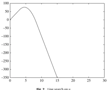
Fig. 2. Line search onu.

Letg

(α)

=

Θ

(

uk

+

α

1uk

;

rj

,

zk

)

, whereΘ

(

·;

rj

,

zk

)

is defined as in(3.5). Theng0

(α)

= ∇

uΘ

(

uk

+

α

1uk

;

rj

,

zk

)

T1uk. We

perform the line search in the interval

[

0

, α

1

]

. Here

α

1can be 1 or a number chosen according to the previous iteration. We

will use the four valuesg

(

0

)

,g0

₍

₀

₎

_,_g

_(α

1

)

andg0

(α

1

)

to construct a curve and use its maximum to approximate the maximum

ofg

(α)

. Normally, an interpolation polynomial can be used as an approximate curve. But this approach does not work very

well here. In our implementation for all test problems, we observed that all functionsg

(α)

had a very similar behaviour

as that plotted inFig. 2, that is, its upward side and downward side were both very steep, and when

α

was away from the

maximum ofg

(α)

,g

(α)

was nearly a linear function. Based on this observation, we construct a piecewise linear–quadratic

approximate functionh

(α)

which is assumed to be linear in the intervals

[

0

,

t0

]

and

[t

1

, α

1

]

, and quadratic in

[t

0

,

t1

]

, i.e.

h

(α)

=







g

(

0

)

+

g0

(

0

)α,

α

∈ [

0

,

t0

),

b0

+

b1

α

+

b2

α

2

,

α

∈ [t

0

,

t1

),

g

(α

1

)

+

g0

(α

1

)(α

−

α

1

), α

∈ [t

1

, α

1

]

.

(3.15)

Although the piecewise linear–quadratic approximation(3.15)performs well in our experiments, we have not been able

to give any analytical justification. Let

ζ

be the intersection point of the two lines defined by the first and third equations in

(3.15). It is noticed thatt0

=

ζ/

3 is an appropriate choice generally. So we are left to determineb0,b1,b2andt1, and this

can be done by imposing the following continuity conditions att0andt1:

g

(

0

)

+

g0

(

0

)

t0

=

b0

+

b1t0

+

b2t02

,

g0

(

0

)

=

b1

+

2b2t0

,

g

(α

1

)

+

g0

(α

1

)(

t1

−

α

1

)

=

b0

+

b1t1

+

b2t12

,

g0

(α

1

)

=

b1

+

2b2t1

.

(3.16)

The system(3.16)has a closed form solution which can be derived by a few steps of algebraic manipulations. With the

coefficients ofh

(α)

determined above, we can find the maximum ofh

(α)

, which is

α

¯

= −

b1

2b2.

In the following two cases, we do not perform the line search process described above, but simply choose

α

₁ as the

step-length:

(i) g

(α

1

)

≥

g

(

0

)

+

0

.

5g0

(

0

)α

1

;

(ii) g0

(α

1

)

≥ −

0

.

1g0

(

0

).

Intuitively, case (i) shows thatg

(α

1

)

is large enough, while case (ii) implies that

α

1is either on the upward side or is not too

far down from the maximum.

Our line search subroutine goes as follows.

Algorithm 3.2.

Step 0. Set

α

1

=

γ σ

(

γ

depends on the size of the problem, e.g.

γ

=

√

nS). Computeg

(

0

)

,g0

(

0

)

,g

(α

1

)

andg0

(α

1

)

. Set count

=

1.

Step 1. If at least one of the conditions (i) and (ii) is satisfied, orcount

≥

3, stop; Otherwise, go to Step 2.

Step 2. Solve(3.16). Set

α

1

= −

₂b_b1₂, andcount

=

count

+

1; go to Step 1.

Here

σ

=

1

/(

1

+

δ)

, where

δ

2_{is the left-hand side quantity in}_(3.12)_{. In our experiment, ‘‘}_count_{’’ seldom reaches the}

(9)

Table 1

Randomly generated stochastic linear programming test problems.

Problem name Number of stages (T) Number of scenarios (S) Nonanticipativity constraints Size of the problemm×n

LP1 2 6 20 146×48 LP2 3 6 24 168×54 LP3 3 16 105 681×208 LP4 3 16 192 1248×320 LP5 5 32 483 2595×672 LP6 4 54 808 4102×1080 LP7 5 256 5124 24 836×7168

4. Test problems and numerical results

Algorithms 2.1and3.1are programmed inMatlabversion 5.3 on a personal computer with Intel Xeon 3.20 GHz processor running the Linux operating system. In this section, we report some preliminary numerical results on the algorithms applied

to some multistage stochastic programming test problems. For all test problems, we use 10−3as the accuracy tolerance

forAlgorithm 2.1, and 10−6_{for the barrier parameter in}_{Algorithm 3.1}_.

Since the two algorithms use different stopping criteria and the exact optimal solutions are not known, comparison of the objective values and constraints violation are made.

In the following tables, NIT and NSS stand for the number of iterations and the number of scenario subproblems solved,

respectively. RNC and VIC represent thel2norms of the residue of the nonanticipativity constraints and the violation of the

inequality constraints respectively. CT is the computational time spent, which is measured in seconds. OBF is the optimal

value of the objective function(1.5). ForAlgorithm 2.1, NIT is always the same as NSS. SinceAlgorithm 3.1is an interior

point method, VIC is always zero forAlgorithm 3.1. Thus, NSS and VIC are not listed forAlgorithms 2.1and3.1respectively.

4.1. The stochastic linear programs with coefficients generated by random number generators

We formulate the programs as in [21], and they have the following form:

min c₀Tx

+

c₁Ty1

+ · · · +

cTTyT (4.1) s.t. x

∈ <

n0

,

_y t

∈ <

nt

,

t

=

1

, . . . ,

T l0

≤

x

≤

u0

,

lt

≤

yt

≤

ut

,

t

=

1

, . . . ,

T A00x

≤

b0

∈ <

m0 (4.2) A10x

+

A11y1

≤

b1

∈ <

m1

· · ·

AT0x

+

AT1y1

+ · · · +

ATTyT

≤

bT

∈ <

mT

.

(4.3) Letn

=

P

T t=0nt andm

=

P

T

t=0mt. For simplicity, we suppose that all scenarios occur with the same probability. The

coefficients in(4.1)are

c

=

(

c0

,

c1

, . . . ,

cT

)

T

=

(

−e

0

,

−e

1

, . . . ,

−e

T

)

T

,

(4.4)

whereet

(

t

=

0

,

1

, . . . ,

T

)

is the vector of ones with dimensionnt. Fort

=

0

,

1

, . . . ,

T, we assume that all components of

ltandutare 0 and 100 respectively. We assume that all the coefficients from stage 1 onward are random variables. For each

staget

=

1

, . . . ,

T, we assume

(

At0

, . . . ,

Att

,

bt

)

hasStrealizations. Realizations of each entry ofAtiare sampled from the

uniform distribution on the interval

[−

0

.

5

,

0

.

5

]

. In order to keep(4.2)–(4.3)consistent, realizations ofbtare generated by

bt

=

At0e0

+

At1e1

+ · · · +

Attet

+ ˆ

bt, whereb

ˆ

t

∈ <

mtis a vector with all its entries chosen from a uniform distribution on

the interval

[

0

,

1

]

. Thus,z

=

(

e0

,

e1

, . . . ,

eT

)

is feasible for the program.

With different values ofn,m,T and S, we generate a set of multistage stochastic linear test problems, which are

summarized inTable 1. Our numerical results forAlgorithms 2.1and3.1are listed inTables 2and3respectively, where

Algorithm 2.1is terminated if the computational time is greater than 80,000 s, whereasAlgorithm 3.1is terminated if the

computational time is greater than 30,000 s. For LP7, we are not able to solve the problems byAlgorithm 2.1within the

given time limit after trying several

β

’s.

From their experiments forAlgorithm 2.1, Helgason and Wallace [14] observed that the penalty parameter

β

should be

as small as possible, provided it is large enough to guarantee convergence. In order to observe how the penalty parameter

β

affects the algorithms, we select three different values of

β

to testAlgorithms 2.1and3.1. The numerical results are listed

inTable 4, where the computational time ofAlgorithm 2.1exceeds the limit for LP6 when

β

=

1, and for LP7 for all the

selected

β

’s. The computational time ofAlgorithm 3.1exceeds the limit for LP7 when

β

=

10−3_.

We observe that from our implementation ofAlgorithm 2.1, small penalty parameters need not always produce better

results. Indeed, for most of the problems,

β

=

0

.

1 performs better than

β

=

0

.

01 in terms of CT time. But varying

β

does

not have a substantial influence on the performance ofAlgorithm 3.1. This is presumably due to the powerful effect of the

(10)

Table 2

Numerical results reported byAlgorithm 2.1for problems inTable 1.

Problem β NIT (NSS) RNC VIC CT OBF

LP1 0.1 364 3.10e−03 3.30e−15 148.39 −175.8469 LP2 0.1 278 3.22e−03 5.04e−15 119.92 −178.8426 LP3 1 4176 8.30e−04 1.80e−14 6140.11 −198.7202 LP4 0.1 1027 2.49e−03 1.30e−13 2599.65 −209.0337 LP5 0.1 5189 2.34e−03 1.45e−13 29 820.43 −408.3469 LP6 0.1 5611 4.10e−03 2.62e−14 37 204.17 −126.3110 LP7 Table 3

Problem β NIT NSS RNC CT OBF

LP1 5×10−3 ₁₇ ₃₇ _1.56e₋₀₉ _5.92 ₋_175.8471 LP2 5×10−3 ₃₅ ₅₈ _1.13e₋₁₀ _8.80 ₋_178.8348 LP3 5×10−3 ₄₉ ₇₀ _1.55e₋₀₉ _35.17 ₋_198.7540 LP4 10−5 ₅₇ ₈₈ _9.87e₋₀₈ _74.61 ₋_209.0342 LP5 10−5 ₇₉ ₁₁₂ _2.39e₋₀₅ _186.68 ₋_408.3594 LP6 5×10−3 ₁₃₅ ₁₈₂ _1.56e₋₀₉ _454.43 ₋_126.3128 LP7 10−5 ₂₉₃ ₅₆₀ _2.20e₋₀₈ _{11 616.03} ₋_619.6291 Table 4

Computational time taken to solve the problems inTable 1for differentβ.

Problem Algorithm 2.1(in s) Algorithm 3.1(in s)

β=0.01 β=0.1 β=1 β=10−3 _β₌₁₀−4 _β₌₁₀−5 LP1 180.59 148.39 357.92 6.31 7.31 8.61 LP2 122.23 119.92 681.92 8.75 9.99 11.31 LP3 8 200.42 11 530.47 6 140.11 35.31 36.19 41.82 LP4 8 212.74 2 599.65 18 613.95 76.63 79.16 74.61 LP5 32 746.13 29 820.43 58 825.20 262.21 209.55 186.68 LP6 38 699.68 37 204.17 480.99 497.25 526.64 LP7 12 565.36 11 616.03

4.2. A multistage production planning problem

In order to meet random demands for its products over several time periods, a factory must decide on a production schedule to increase or decrease its production activity in different periods. The details on modeling this problem as an

optimization problem can be found in [22]. As a test problem for multistage stochastic program with general recourse, it is

described with complete data in [23]. At each stage, the decision is made as a function of the decisions and realizations of the

random variables of the previous stages, and the expected future outcomes of the random variables. It can be thought of as a dynamic programming problem. But due to the high dimensionality of the state space of the problem, it is computationally difficult to solve it by a dynamic programming based method.

A solution for this problem has been presented in [22]. In this paper, by using scenario analysis technique, we reformulate

it as a 5-stage stochastic program with recourse. Our model is as follows. min 4

X

t=1 2

X

j=1

(

cj

+

q0j,t

+

(

−

1

)

t a3je +

₎

xj,t

+

4

X

t=1 3

X

i=1 diui,t

+

3

X

t=1

(

e+

+

e−

)w

−_t

+

4

X

t=1 2

X

j=1

(

q+_j_,_t

+

q_j0_,_t

)

Ey+_j_,_t

−

4

X

t=1 2

X

j=1 q0_j_,_tE

ξ

j,t (4.5) stage-0











2

X

j=1 a3j

(

xj,t

−

xj,t+1

)

−

w

− t

≤

0

,

t

=

1

, . . . ,

3 2

X

j=1 aijxj,t

−

ui,t

≤

bi,t

,

i

=

1

, . . . ,

3

;

t

=

1

, . . . ,

4 ui,t

≤

fi,t

,

i

=

1

, . . . ,

3

;

t

=

1

, . . . ,

4 xj,t

≥

0

,

j

=

1

,

2

;

t

=

1

, . . . ,

4 ui,t

≥

0

,

i

=

1

, . . . ,

3

;

t

=

1

, . . . ,

4

w

− t

≥

0

,

t

=

1

, . . . ,

3 (4.6)

(11)

Table 5

The solution for the multistage production planning problem.

t=1 t=2 t=3 t=4 x: j=1 335.90 284.10 444.34 403.85 j=2 563.18 585.39 398.85 376.92 u: i=1 159.54 63.32 0.00 0.00 i=2 0.00 0.00 0.00 0.00 i=3 450.00 450.00 375.00 350.00 w− : 0.00 825.00 275.00 Table 6

Two sets of production and manpower planning problems.

Problem name Number of stages Number of scenarios Nonanticipativity constraints Size of the problem row×column

PP1 3 16 189 701×240 PP2 3 256 3285 11 477×3840 PP3 5 256 7233 24 129×7936 MP1 3 16 117 549×240 MP2 3 64 525 2253×960 MP3 5 16 249 1065×432 MP4 5 256 4869 17 925×6912 Table 7

Problem β NIT (NSS) RNC VIC CT OBF

PP1 0.5 131 4.36e−03 3.27e−13 194.50 243 958.6404 PP2 0.1 142 1.76e−03 5.29e−12 3 542.23 247 373.7902 PP3 5×10−3 ₁₉₇ _1.62e₋₀₂ _1.73e₋₁₀ _{15 622.59} _{594 574.8905} MP1 10−3 ₃₃₀ _1.60e₋₀₃ _5.12e₋₁₂ _503.26 _{80 628.8417} MP2 10−4 ₇₉₈ _4.70e₋₀₃ _1.55e₋₁₁ _{5 348.49} _{80 664.8142} MP3 10−4 ₈₃ _4.45e₋₀₄ _8.76e₋₁₂ _311.39 _{85 830.4461} MP4 10−4 ₄₀₆ _1.93e₋₀₂ _3.71e₋₁₁ _{19 940.98} _{86 149.2761} other stages







xj,1

+

y + j,1

≥

ξ

j,1

,

j

=

1

,

2 xj,t−1

+

xj,t

+

y + j,t−1

+

y + j,t

≥

ξ

j,t−1

+

ξ

j,t

,

j

=

1

,

2

;

t

=

2

,

3

,

4 y+_j_,_t

≥

0

,

j

=

1

,

2

;

t

=

1

, . . . ,

4 (4.7) whereq0_j_,_t

=

P

4 i=tq −

i,t, and the coefficients are given in [23]. In the model,xj,t,ui,t

(

j

=

1

,

2

;

t

=

1

, . . . ,

4

)

,

w

−

t

(

t

=

1

,

2

,

3

)

are variables in the first stage,y+_j_,_t

(

j

=

1

,

2

;

t

=

1

, . . . ,

4

)

are variables in subsequent stages, wherexj,t is the amount of

productjupon time periodt,ui,t is the extra capacity of production activityiupon time periodt,

w

−t is the change in

utilization of production activity 3 fromt tot

+

1,y+_j_,_t is the amount of purchased deficit productjupon time periodt

(see [23]). The original random variables

ξ

j,t(j

=

1

,

2

;

t

=

1

, . . . ,

4) are continuously distributed, which represent the

demands for productsj

(

j

=

1

,

2

)

upon time periodst

(

t

=

1

, . . . ,

4

)

. We divide the support of each random variable

ξ

j,tinto several intervals (say,Ijl,t

(

l

=

1

, . . . ,

L

)

) with the same probabilities, and calculate

ξ

l

j,t

=

E{

ξ

j,t

|

Ijl,t

}

. Then the

random variable

ξ

j,tis approximated by the discrete random variable with realizations

ξ

jl,t

(

l

=

1

, . . . ,

L

)

and corresponding

probability 1

/

L. By eliminating the equality constraints, we derive a deterministic equivalent of the 5-stage stochastic

program with recourse, which has only inequality constraints.

The problem(4.5)–(4.7)is a 5-stage problem with 31 variables (23 variables for the first stage and 2 for each subsequent

stage) and 66 constraints (50 constraints for the first stage and 4 for each subsequent stage). By using the discrete random

variable with two realizations (L

=

2) to approximate each continuous random variable, the problem is a stochastic program

with 256 scenarios.

As a stochastic program, this problem has been solved in [22], the solution was reported and compared with that of the

deterministic program obtained by setting the stochastic variables equal to their expected values (see [22] for details). For a

comparison, we report our results inTable 5from solving the formulation(1.5)–(1.7). The solutions given byAlgorithms 2.1

and3.1are totally the same up to two digits after the decimal point. Some small-size reformulations are also used to test

Algorithms 2.1and3.1. The size of the problems are listed inTable 6. The numerical results are listed inTables 7and8. 4.3. The manpower planning problem

An employer must decide upon the level of regular staff at various skill levels. In order to meet the random demand for services at minimum cost, the employer should make a schedule for temporary external manpower or regular staff

(12)

Table 8

Problem β NIT NSS RNC CT OBF

PP1 10−4 ₂₆ ₄₂ _2.68e₋₀₇ _22.03 _{243 958.6110} PP2 10−4 ₂₀ ₄₁ _4.33e₋₀₈ _540.49 _{247 373.7894} PP3 10−4 ₂₅ ₄₂ _1.66e₋₀₇ _1656.56 _{594 575.0862} MP1 5×10−5 ₃₄ ₅₈ _2.95e₋₀₈ _24.72 _{80 628.8422} MP2 10−6 ₃₉ ₆₄ _4.20e₋₀₄ _123.11 _{80 664.8127} MP3 10−5 ₁₇ ₂₉ _2.30e₋₀₉ _23.80 _{85 830.4465} MP4 10−6 ₅₂ ₉₅ _2.08e₋₀₇ _2043.56 _{86 149.2823} Table 9

Numerical results for a stochastic nonlinear program with constraint(4.11).

Algorithm NIT NSS RNC VIC CT OBF

Algorithm 2.1 330 330 2.06e−03 4.98e−15 280.83 −149.2547

Algorithm 3.1 11 24 7.57e−10 0 7.33 −149.2470

overtime. This problem can be modeled as a multistage stochastic program with general recourse, which is described in [23].

Comparing to the production planning problem above, the formulation of this problem is simpler and more straightforward. This problem can be formulated as following:

min 3

X

j=1 cjxj

+

3

X

j=1 T

X

t=1 E

(

qjyj,t

+

rjzj,t

)

(4.8) stage-0

xj

≥

0

,

j

=

1

,

2

,

3 (4.9) stage-t











3

X

j=1

(α

txj

+

yj,t

+

zj,t

)

≥

ξ

t yj,t

≥

0

,

j

=

1

,

2

,

3 0

.

2

α

txj

−

yj,t

≥

0

,

j

=

1

,

2

,

3 zj,t

≥

0

,

j

=

1

,

2

,

3

γ

j−1

(

xj−1

+

yj−1,t

+

zj−1,t

)

−

(

xj

+

yj,t

+

zj,t

)

≥

0

,

j

=

1

,

2

,

3 (4.10) t

=

1

, . . . ,

T

wherexj

(

j

=

1

,

2

,

3

)

are variables in the first stage (that is, stage-0),yj,t andzj,t

(

j

=

1

,

2

,

3

)

are variables in thet

+

1

stage (stage-t). In the formulation,xjis the amount of regular staff at skill levelj,yj,tandzj,t are the amounts of regular

staff overtime and temporary staff at skill leveljin stage-t, respectively. The stage-trandom variable

ξ

tis the demand for

service in the stage, which is assumed to be independent on random variables in other stages and has a normal distribution N

(

µ

¯

_t

,

σ

¯

2

t

)

with

σ

¯

t2

=

10

µ

¯

t. The random variables are alike approximated by discrete random variables with equiprobability

realizations.

We have tested four problems with different sizes (seeTable 6), the numerical results are listed inTables 7and8.

4.4. Multistage stochastic nonlinear test problems

Algorithms 2.1and3.1are also used to solve some multistage stochastic nonlinear test problems. The first test problem

is derived by adding a nonlinear term1₂x2₁

+

exp

(

x2

)

to the objective function and a nonlinear inequality constraint

sin

(

x1

)

+

x22

+

exp

(

1

+

x3

)

≤

25 (4.11)

in stage-0 of LP2. Herex

=

(

x1

,

x2

,

x3

)

is the stage-0 variable. Note that LP2 is a 3-stage 6-scenario stochastic linear program,

and there are 3 variables and 2 constraints for each stage, 3 realizations for stage 1 and 2 realizations for stage 2, the generated

problem is a 3-stage 6-scenario stochastic nonlinear program. The numerical results for this problem are listed inTable 9.

The other test problems are derived by adding 4 nonlinear constraints to LP1, LP2, LP3 and LP4. The first two constraints are x2₁

+

x2₂

−

2x3

≤

15

,

(4.12) 3x1

+

x32

+

1 2x 2 3

≤

160

,

(4.13)

which are related to stage-0 of the problems. The other two constraints are added to stage-1 and stage-2. For LP2, LP3 and LP4, the first of the following constraints is added to stage-1 and the second is added to stage-2:

(13)

Table 10

Numerical results for stochastic nonlinear programs with constraints(4.12)–(4.15).

Algorithm Problem NIT NSS RNC VIC CT OBF

NLP1 249 249 3.83e−03 1.13e−12 126.39 −33.7382

Algorithm 2.1 NLP2 116 116 2.83e−03 8.37e−13 79.36 −40.7556

β=0.1 NLP3 267 267 4.57e−03 6.03e−12 502.46 −41.4489 NLP4 340 340 3.65e−03 3.01e−12 1186.70 −52.4869 NLP1 24 60 1.63e−09 0 36.86 −33.7373 Algorithm 3.1 NLP2 19 36 1.62e−09 0 18.67 −40.7544 β=0.005 NLP3 45 75 4.35e−11 0 107.27 −41.4499 NLP4 70 116 2.29e−11 0 235.74 −52.4852 ¯ n1

X

i=0 d1iy21i

≤

300

,

(4.14) ¯ n2

X

i=0 d2iy32i

≤

750

.

(4.15)

For LP1, both the constraints above are added to stage-1. Heren

¯

j

(

j

=

1

,

2

)

is the number of variables up to thejth stage, i.e.,

¯

nj

=

P

j

t=0nt;dji

(

j

=

1

,

2

)

are random coefficients; andyti(t

=

1

,

2) is thei-component of thet-stage variableyt. For each

(

j

,

i

)

, we generatedjiaccording to the uniform distribution on

[

0

,

1

]

. The numerical results are presented inTable 10. The

problem with nonlinear constraints added to the linear problem LPiis named NLPi. In our experiments, we used different

values of

β

for each algorithm. Here for each algorithm we only report the best value of

β

and the corresponding numerical

results.

4.5. Observations and remarks

The main difference betweenAlgorithms 2.1and3.1is thatAlgorithm 3.1smoothes the Lagrangian dual function by

barrier functions and the resulting problem is solved by a second-order method, namely, the Newton method. From the results of our preliminary numerical experiments, one can see obvious improvements in terms of the solution quality such as the residue of the nonanticipativity constraints (RNC) and the computational time. These numerical results, together

with the strong convergence properties established in [20], demonstrate the promising potential of the barrier progressive

hedging method.

Acknowledgements

We are grateful to two anonymous referees for their serious reading and insightful comments and suggestions on the initial version of the paper. We also thank the editor for his suggestions and kind help in editing the paper.

References

[1] J.R. Birge, F. Louveaux, Introduction to Stochastic Programming, Springer-Verlag, 1997. [2] P. Kall, S.W. Wallace, Stochastic Programming, John Wiley & Sons, NY, 1994.

[3] A. Berkelaar, C. Dert, B. Oldenkamp, S. Zhang, A primal-dual decomposition-based interior point approach to two-stage stochastic linear programming, Oper. Res. 50 (2002) 904–915.

[4] J.R. Birge, Current trends in stochastic programming computation and applications, Technical Report 95-15, Department of Industrial and Operations Engineering, University of Michigan, 1995.

[5] H.I. Gassmann, MSLiP: A computer code for the multistage stochastic linear programming problem, Math. Program. 47 (1990) 407–423.

[6] J. Mayer, Stochastic Linear Programming Algorithms: A Comparison based on a Model Management System, Gordon and Breach Science Publishers, 1998.

[7] A. Ruszczyński, Some advances in decomposition methods for stochastic linear programming, in: Stochastic Programming, State of the Art, 1998 (Vancouver, BC), Ann. Oper. Res. 85 (1999) 153–172.

[8] J. Sun, X. Liu, Scenario formulation of stochastic linear programs and the homogeneous self-dual interior point method, INFORMS J. Comput. 18 (2006) 444–454.

[9] G. Zhao, Interior-point methods with decomposition for solving large-scale linear programs, J. Optim. Theory Appl. 102 (1999) 169–192. [10] G. Zhao, A log-barrier method with Benders decomposition for solving two-stage stochastic programs, Math. Program. 90 (2001) 507–536. [11] R.T. Rockafellar, R.J.-B. Wets, Scenarios and policy aggregation in optimization under uncertainty, Math. Oper. Res. 16 (1991) 119–147.

[12] N.J. Berland, K.K. Haugen, Mixing stochastic dynamic programming and scenario aggregation, in: Stochastic Programming, Algorithms and Models (Lillehammer, 1994), Ann. Oper. Res. 64 (1996) 1–19.

[13] J.M. Mulvey, H. Vladimirou, Applying the progressive hedging algorithm to stochastic generalized networks, Ann. Oper. Res. 31 (1991) 399–424. [14] T. Helgason, S.W. Wallace, Approximate scenario solutions in the progressive hedging algorithm, Ann. Oper. Res. 31 (1991) 425–444.

[15] B.J. Chun, S.M. Robinson, Scenario analysis via bundle decomposition, Ann. Oper. Res. 56 (1995) 39–63.

[16] A. Ruszczyński, Parallel decomposition of multistage stochastic programming problems, Math. Program. 58 (1993) 201–228.

[17] A. Ruszczyński, On convergence of an augmented Lagrangian decomposition method for sparse convex optimization, Math. Oper. Res. 20 (1995) 634–656.

[18] X. Liu, M. Fukushima, Parallelizable preprocessing method for multistage stochastic programming problems, J. Optim. Theory Appl. 131 (2006) 327–346.