Inference for Parameters Defined by Moment Inequalities: A Recommended Moment Selection Procedure

Inference for Parameters Defined by Moment Inequalities:

A Recommended Moment Selection Procedure

By

Donald W.K. Andrews and Panle Jia

September 2008

Revised August 2011

COWLES FOUNDATION DISCUSSION PAPER NO. 1676R

COWLES FOUNDATION FOR RESEARCH IN ECONOMICS

YALE UNIVERSITY

Box 208281

Inference for Parameters De…ned by

Moment Inequalities: A Recommended

Moment Selection Procedure

Donald W. K. Andrews

Cowles Foundation for Research in Economics

Yale University

Panle Jia

Department of Economics

MIT

June 2008

Revised: May 2011

Andrews gratefully acknowledges the research support of the National

Science Foundation via grant SES-0751517. The authors thank Steve

Berry for numerous discussions and comments. The authors also thank

the co-editor, three referees, and Michael Wolf for very helpful

comments.

Abstract

This paper is concerned with tests and con…dence intervals for parameters that are not necessarily identi…ed and are de…ned by moment inequalities. In the literature, di¤erent test statistics, critical value methods, and implementation methods (i.e., the asymptotic distribution versus the bootstrap) have been proposed. In this paper, we compare these methods. We provide a recommended test statistic, moment selection critical value method, and implementation method. We provide data-dependent proce-dures for choosing the key moment selection tuning parameter and a size-correction factor :

Keywords: Asymptotic size, asymptotic power, bootstrap, con…dence set, generalized moment selection, moment inequalities, partial identi…cation, re…ned moment selection, test, unidenti…ed parameter.

1

Introduction

This paper considers inference in moment inequality models with parameters that need not be identi…ed. We focus on con…dence sets for the true parameter, as opposed to the identi…ed set. We construct con…dence sets (CS’s) by inverting Anderson-Rubin-type test statistics. We consider a class of such statistics and a class of generalized moment selection (GMS) critical values. This approach follows Imbens and Manski (2004), Chernozhukov, Hong, and Tamer (2007) (CHT), Andrews and Guggenberger (2009) (AG), Andrews and Soares (2010) (AS), and other papers.

GMS and subsampling tests and CS’s are the only methods in the literature that apply to arbitrary moment functions and have been shown to have correct asymptotic size in a uniform sense, see AG, AS, and Romano and Shaikh (2008). AS and Bugni (2010) show that GMS tests dominate subsampling tests in terms of asymptotic size and power properties. In addition, in our experience based on simulation results, sub-sampling tests often are substantially under-sized in …nite samples in moment inequality testing problems. Hence, we focus on GMS critical values.

GMS tests and CS’s depend on a test statistic functionS;a critical value function';

and a tuning parameter :In this paper we determine a combination that performs well in terms of size and power and can be recommended for general use. To do so, we consider asymptotics in which equals a …nite constant plus op(1); rather than asymptotics in which _{! 1} as n_{! 1}; as has been considered elsewhere in the literature.1

We …nd that anadjusted Gaussian quasi-likelihood ratio (AQLR) test statistic com-bined with a “t-test moment selection” critical value performs very well in terms of asymptotic average power compared to other choices considered in the literature.2 _We develop data-dependent methods of selecting and a size-correction factor and show that they yield very good asymptotic and …nite-sample size and power. We provide a table that makes them easy to implement in practice for up to ten moment inequalities. We show that with i.i.d. observations bootstrap critical values out-perform those based on the asymptotic-distribution in terms of …nite-sample size. We also show that the bootstrap version of the AQLR test performs similarly in terms of null rejection probabilities and power to an analogous test based on the empirical likelihood ratio (ELR) statistic. The AQLR-based test is noticeably faster to compute than the

ELR-1_{The theoretical arguments mentioned in the preceding paragraph rely on}

! 1asymptotics. 2_{The “adjustment”in the AQLR test statistic is designed to handle singular asymptotic correlation} matrices of the sample moment functions.

based test and avoids computational convergence problems that can arise with the ELR statistic when the correlation matrix of the moment conditions is singular.

The asymptotic results of the paper apply to i.i.d. and time series data and to mo-ment functions that are based on preliminary estimators of point-identi…ed parameters. In short, the contribution of this paper relative to the literature is to compare moment inequality tests, determine a recommended test, and provide data-dependent tuning parameters.

The remainder of the paper is organized as follows. Section 2 introduces the model and describes the recommended con…dence set and test. Section 3 de…nes the di¤erent test statistics and critical values that are compared in the paper. Section 4 provides the numerical comparisons of the tests based on asymptotic average power. Section 5 describes how the recommended data-dependent tuning parameterband size-correction factor _b are determined and provides numerical results assessing their performance. Section 6 gives …nite-sample results.

Andrews and Jia (2008) (AJ2) provides Supplemental Material that includes: (i) the asymptotic results that are utilized in this paper, (ii) details concerning the numerical results given here, and (iii) additional numerical results.

Let R+ = fx 2 R : x 0g; R++ = fx 2 R : x > 0g; R+;1 = R+ [ f+1g;

Kp _{=K ::: K (with pcopies) for any set K; and 0}

p = (0; :::;0)0 2Rp:

2

Model and Recommended Con…dence Set

The moment inequality model is speci…ed as follows. The true value 0 (2 Rd) is assumed to satisfy the moment conditions:

EF0mj(Wi; 0) 0for j = 1; :::; p; (2.1)

where _fmj(; ) :j = 1; :::; pg are known real-valued moment functions andfWi :i 1g are i.i.d. or stationary random vectors with joint distribution F0:The observed sample is _fWi : i ng: The true value 0 is not necessarily identi…ed. The results also apply when the moment functions in (2.1) depend on a parameter ; i.e., when they are of the form _fmj(Wi; ; ) : j pg; and a preliminary consistent and asymptotically normal estimator _bn( 0) of exists, see AJ2. In addition, the asymptotic results in AJ2 allow for moment equalities as well as moment inequalities.

We are interested in tests and con…dence sets (CS’s) for the true value 0:We consider a con…dence set obtained by inverting a test. The test is based on a test statistic Tn( 0) for testing H0 : = 0: The nominal level1 CS for is

CSn =f 2 :Tn( ) cn( )g; (2.2)

where cn( ) is a data-dependent critical value.3

We now describe the recommended test statistic and critical value. The justi…ca-tions for these recommendajusti…ca-tions are described below and are given in detail in AJ2. The recommended test statistic is an adjusted quasi-likelihood ratio (AQLR) statistic,

TAQLR;n( ); that is a function of the sample moment conditions, n1=2mn( ); and an estimator of their asymptotic variance, bn( ):

TAQLR;n( ) = S2A(n1=2mn( );bn( )) = inf t2R₊p_;1 (n1=2mn( ) t)0en1( )(n1=2mn( ) t); where mn( ) = (mn;1( ); :::; mn;p( ))0; mn;j( ) =n 1 n X i=1 mj(Wi; ) for j p; e_n( ) = bn( ) + maxf" det(bn( ));0gDbn( ); "=:012; b Dn( ) = Diag(bn( )); bn( ) =Dbn1=2( )bn( )Dbn1=2( ); (2.3) and Diag( )denotes the diagonal matrix based on the matrix :4 Note that the weight matrix en( )depends only onbn( )and henceTAQLR;n( )can be written as a function of

(mn( );bn( )):The functionS2A( )is an adjusted version of the QLR functionS2( )that appears in Section 3. The adjustment is designed to handle singular variance matrices. Speci…cally, the matrix en( ) equals the asymptotic variance matrix estimator bn( ) with an adjustment that ensures that en( ) is always nonsingular and is invariant to scale changes in the moment functions. The matrix bn( ) is the correlation matrix that corresponds to bn( ):

3_{When is in the interior of the identi…ed set, it may be the case thatT}

n( ) = 0andcn( ) = 0:In

consequence, it is important that the inequality in the de…nition ofCSn is ;not< :

4_{The constant"=:012was determined numerically based on an average asymptotic power criterion.} See Section 6.2 of AJ2 for details.

When the observations are i.i.d. and no parameter appears, we take bn( ) = n 1 n X i=1 (m(Wi; ) mn( ))(m(Wi; ) mn( ))0; where m(Wi; ) = (m1(Wi; ); :::; mp(Wi; ))0: (2.4)

With temporally dependent observations or when a preliminary estimator of a parameter appears, a di¤erent de…nition of bn( ) often is required, see AJ2. For example, with dependent observations, a heteroskedasticity and autocorrelation consistent (HAC) estimator may be required.

The test statisticTAQLR;n( )is computed using a quadratic programming algorithm. Such algorithms are built into GAUSS and Matlab. They are very fast even when p is large. For example, to compute the AQLR test statistic 100,000 times takes 2:6; 2:9;

and 4:7 seconds when p = 2; 4; and 10; respectively, using GAUSS on a PC with a 3.4 GHz processor.5

A moment selection critical value that utilizes a data-dependent tuning parameter _b and size-correction factor _b is referred to as a re…ned moment selection (RMS) critical value. Our recommended RMS critical value is

cn( ) =cn( ;b) +b; (2.5) wherecn( ;b)is the1 quantile of a bootstrap (or “asymptotic normal”) distribution of a moment selection version of TAQLR;n( ) and b is a data-dependent size-correction factor. For i.i.d. data, we recommend using a nonparametric bootstrap version of

cn( ;b): For dependent data, either a block bootstrap or an asymptotic normal version can be applied.

We now describe the bootstrap version of cn( ;b):LetfWi;r :i ng forr= 1; :::; R denote R bootstrap samples of size n (i.i.d. across samples), such as nonparametric i.i.d. bootstrap samples in an i.i.d. scenario or block bootstrap samples in a time series scenario, where R is large. De…ne the bootstrap variance matrix estimator b_n;r( ) as b_n( ) is de…ned (e.g., as in (2.4) in the i.i.d. case) with _fW_i;r : i n_g in place of fWi :i ng throughout.6 The p-vectors of re-centered bootstrap sample moments and

5_{In our experience, the GAUSS 9.0 quadratic programming procedure “qprog” is much faster than} the Matlab 7 procedure “quadprog.”

6_{Note that when a preliminary consistent estimator of a parameter appears, the bootstrap moment} conditions need to be based on a bootstrap estimator of this preliminary estimator. In such cases, the

p pbootstrap weight matrices for r = 1; :::; R are de…ned by

m_n;r( ) = n1=2 m_n;r( ) mn( ) and

e_n;r( ) = b_n;r( ) + max_f" det(b_n;r( ));0_gDb_n;r( ); where "=:012;

b D_n;r( ) = Diag(b_n;r( )); and bn;r( ) =Dbn;r( ) 1=2_b n;r( )Dbn;r( ) 1=2 : (2.6)

The idea behind the RMS critical value is to compute the critical value using only those moment inequalities that have a noticeable e¤ect on the asymptotic null distri-bution of the test statistic. Note that moment inequalities that have large positive population means have little or no e¤ect on the asymptotic null distribution. Our pre-ferred RMS procedure employs element-by-element t-tests of the null hypothesis that the mean of mn;j( ) is zero versus the alternative that it is positive for j = 1; :::; p: The

j-th moment inequality is selected if

n1=2_m n;j( )

bn;j( ) b

; (2.7)

whereb2

n;j( )is the(j; j)element of bn( )forj = 1; :::; pandbis a data-dependent tun-ing parameter (de…ned in (2.10) below) that plays the role of a critical value in selecttun-ing the moment inequalities. Let p_bdenote the number of selected moment inequalities.

For r= 1; :::; R;letm_n;r( ;p_b) denote thep_b-sub-vector of m_n;r( ) that includes the p_b

selected moment inequalities.7;8 _{Analogously, let}b

n;r( ;pb)denote the(pb pb)-sub-matrix of b_n;r( ) that consists of the p_bselected moment inequalities. The bootstrap quantity

cn( ;b)is the 1 sample quantile of

fS2A(mn;r( ;pb);bn;r( ;pb)) :r= 1; :::; Rg; (2.8) where S2A(; ) is de…ned as in (2.3) but withpreplaced by p:b

An “asymptotic normal” version of cn( ;b) is obtained by replacing the bootstrap quantities m_n;r( ;p_b) and b_n;r( ;p_b) in (2.8) by b1=2n ( ;bp)Z_r and bn( ;pb); respectively, where bn( ;pb) denotes the (pb pb)-sub-matrix of bn( ) that consists of the bp selected

asymptotic normal version of the critical value may be much quicker to compute. 7_{Note thatm}

n;r( ;pb)depends not only on the number of moments selected,p;b but which moments

are selected. For simplicity, this is suppressed in the notation.

8_{By de…nition,pb 1;i.e., at least one moment must be selected. For speci…city, m}

n;r( ;bp)equals

the last element ofm_n;r( )if no moments are selected via (2.7).

moment inequalities, Z_r i:i:d: N(0_bp; Ipb) for r = 1; :::; R; and fZr : r = 1; :::; Rg are independent of _fWi :i ng conditional on p:b

The tuning parameterbin (2.7) and the size-correction factorbin (2.5) depend on the estimator bn( ) of the asymptotic correlation matrix ( ) of n1=2mn( ): In particular, they depend on bn( ) through a [ 1;1]-valued function (bn( )) that is a measure of the amount of negative dependence in the correlation matrix bn( ):We de…ne

( ) =smallest o¤-diagonal element of ; (2.9)

where is a p p correlation matrix. The moment selection tuning parameter b and the size-correction factor_b are de…ned by

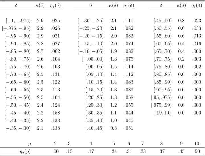
b = (bn( )) and b= 1(bn( )) + 2(p); wherebn( ) = (bn( )): (2.10) Table I provides values of ( ); ₁( ); and 2(p) for 2[ 1;1]and p2 f2;3; :::;10g for tests with level = :05 and CS’s with level 1 = :95: AJ2 provides simulated values of the mean and standard deviation of the asymptotic distribution of cn( ;b): These results, combined with the values of ₁( ) and ₂(p) in Table I, show that the size-correction factor_b typically is small compared tocn( ;b);but not negligible.9

Computation of the ₂(p)values given in Table I by simulation is not easy because it requires computing the (asymptotic) maximum null rejection probability (MNRP) over a large number of null mean vectors and correlation matrices : For this reason, we only provide 2(p) values for p 10: For the correlation matrices, we consider both a …xed grid and randomly generated matrices. For the null mean vectors ₂ Rp_+;1;

computation of the 2(p) values is carried out initially for mean vectors that consist only of 00s and ₁0_{s: Then, the di¤erences are computed between the values obtained}

by maximization over such vectors and the values obtained by maximization over vectors that lie in (i) a …xed full grid, (ii) two partial grids, and (iii) 1,000 or 100,000 randomly generated vectors (depending on the variance matrix). The di¤erences are found to be :0000 in most cases and small ( :0018) in all cases, see AJ2 for details. These results indicate, although do not establish unequivocally, that the maxima over

2Rp_+;1 are obtained at vectors that consist only of 00_{s and 1}0_s:

9_{For example, for p= 10; =I}

10; …ve moment inequalities binding, and …ve moment inequalities

completely slack, the mean and standard deviation of the asymptotic distribution of cn( ;b) are 7:2

In sum, the preferred RMS critical value, cn( );and CS are computed using the fol-lowing steps. One computes (i) bn( ) de…ned in (2.4), (ii)bn( ) =smallest o¤-diagonal element of bn( );(iii) b= (bn( )) using Table I, (iv)b= 1(bn( )) + 2(p)using Table I, (v) the vector of selected moments using (2.7), (vi) the selected bootstrap sample moments, correlation matrices, and weight matrices _f(m_n;r( ;p_b);b_n;r( ;_bp);e_n;r( ;p_b)) :

r = 1; :::; R_g; de…ned in (2.6) with the non-selected moment inequalities omitted, (vii)

cn( ;b); which is the :95 sample quantile of fS2A(mn;r( ;pb); bn;r( ;pb)) : r = 1; :::; Rg (for a test of level:05and a CS of level:95)and (viii)cn( ) =cn( ;b) +b:The preferred RMS con…dence set is computed by determining all the values for which the null hy-pothesis that is the true value is not rejected. For the asymptotic normal version of the recommended RMS critical value, in step (vi) one computes the selected sub-vector and sub-matrix of b1=2n ( ;pb)Zr and bn( ;bp); de…ned in the paragraph following (2.8), and in step (vii) one computes the :95sample quantile with these quantities in place of

m_n;r( ;p_b)and b_n;r( ;p_b); respectively.

To compute the recommended bootstrap RMS test using R =10,000 simulation rep-etitions takes 1:3; 1:5; and2:7seconds when p= 2; 4;and 10; respectively, andn = 250

using GAUSS on a PC with a 3.4 GHz processor. For the “asymptotic normal”version, the times are :20; :25; and :45seconds.

When constructing a CS, if the computation time is burdensome (because one needs to carry out many tests with di¤erent values of as the null value), then a useful approach is to map out the general features of the CS using the “asymptotic normal” version of the MMM/t-Test/ =2.35 test, which is extremely fast to compute, and then switch to the bootstrap version of the recommended RMS test to …nd the boundaries of the CS more precisely.10

10_{The “asymptotic normal” version of the MMM/t-Test/ =2.35 test is de…ned just as the} recom-mended RMS test is de…ned but with(S1; = 2:35; = 0)in place of(S2A;b;b);respectively, whereS1

is de…ned in (3.2), and with the bootstrap replaced by the normal asymptotic distribution. The boot-strap version of this test is much slower to compute than the asymptotic normal version and, hence, we do not recommend that it is used for this purpose. The computation times for the “asymptotic normal”version of the MMM/t-Test/ =2.35 test are:007; :014;and:03seconds whenp= 2;4;and10;

respectively.

3

Test Statistics and Critical Values

We now describe the justi…cation for the recommended RMS test. Details are given in AJ2. The test statistics Tn( ) that we consider are of the form

Tn( ) =S(n1=2mn( );bn( )); (3.1) where S is a real function on (R_{[ f}+_1g)p _V and _V is the space of p p variance matrices. The leading examples ofS are the AQLR functionS2Ade…ned above, the QLR functionS2;which is the same asS2Ain (2.3) but with"= 0(and hence en( ) = bn( )), the modi…ed method of moments (MMM) function S1; and the SumMax functionS3:

S1(m; ) = p X j=1 [mj= j]2 and S3(m; ) = p1 X j=1 [m(j)= (j)]2; (3.2)

where [x] = min_fx;0_g; m = (m1; :::; mp)0; 2j is the jth diagonal element of ;

[m(j)= (j)]2 denotes the jth largest value among f[m`= `]2 : ` = 1; :::; pg; and p1 < p is some speci…ed integer.11;12;13 _{The MMM statisticS}

1 has been used by Pakes, Porter, Ho, and Ishii (2004), CHT, Fan and Park (2007), Romano and Shaikh (2008), AG, AS, and Bugni (2010); the (unadjusted) QLR statistic has been used by AG, AS, and Rosen (2008); and the Max and SumMax statisticsS3 have been used by AG, AS, and Azeem Shaikh.14

We consider the class of GMS critical values discussed in AS. They rely on a tuning parameter and moment selection functions '_j : (R_{[ f}+_1g)p _! R+ for j p; where is the set of all p pcorrelation matrices. The leading examples of '_j are

'(1)_j ( ; ) = ( 0 if j 1 1 if _j >1; ' (2) j ( ; ) = [ ( j 1)]+; ' (3) j ( ; ) = [ j]+; '(4)_j ( ; ) = _j1( _j >1); and '(0)_j ( ; ) = 0 (3.3)

for j p; where [x]+ = maxfx;0g; = ( 1; :::; p)0; is a p p correlation matrix,

11_{When constructing a CS, a natural choice forp}

1 is the dimension dof ;see below.

12_{With the functionsS}

1; S2A;andS3;there is no restriction on the parameter space for the variance

matrix of the moment conditions— can be singular. 13_{Several papers in the literature use a variant ofS}

1that is not invariant to rescaling of the moment

functions (i.e., with j= 1for allj):This is not desirable in terms of the power of the resulting test.

and in '(2)_j and '(4)_j is the tuning parameter : Let'( ; ) = ('₁( ; ); :::; '_p( ; ))0

(for any '_j( ; ) as in (3.3)). CHT, AS, and Bugni (2010) consider the function '(1)_; Canay (2010) considers '(2); AS considers '(3); and Fan and Park (2007) use a non-scale-invariant version of '(4): The function '(1) generates the recommended “moment selection t-test” procedure of (2.7), see AJ2 for details. The function '(0) generates a critical value based on the least-favorable distribution evaluated at an estimator of the true variance matrix : It only depends on the data through the estimation of : It is referred to as the “plug-in” asymptotic (PA) critical value. (No value is needed for this critical value.) Another ' function is the modi…ed moment selection criterion (MMSC) '(5) _{function introduced in AS. It is computationally more expensive than the} functions '(1)_-'(4) _{considered above, but uses all of the information in the p-vector of} moment conditions to decide which moments to select. It is a one-sided version of the information-criterion-based moment selection criterion considered in Andrews (1999). For brevity, we do not de…ne '(5) here, but we consider it below.

For a GMS critical value as in AS, _f = n :n 1g is a sequence of constants that diverges to in…nity as n _{! 1}; such as n = (lnn)1=2: In contrast, for an RMS critical value, _bdoes not go to in…nity asn_{! 1}and is data-dependent. Data-dependence of _b is obtained by taking_b to depend on bn( ): b= (bn( ));where ( ) is an R++-valued function. We justify RMS critical values using asymptotics in which equals a …nite constant plus op(1); rather than asymptotics in which ! 1 as n ! 1: This di¤ers from the asymptotics in other papers in the moment inequality literature.

There are four reasons for using …nite- asymptotics. First, they provide better approximations because is …nite, not in…nite, in any given application. Second, for any given(S; ');they allow one to compute a best value in terms of asymptotic average power, which in turn allows one to compare di¤erent (S; ')functions (each evaluated at its own best value) in terms of asymptotic average power. One cannot determine a best value in terms of asymptotic average power when _{! 1} because asymptotic power is always higher if is smaller, asymptotic size does not depend on ;and …nite-sample size is worse if smaller.15 _{Third, for the recommended (S; ') functions, the} …nite-asymptotic formula for the best value lets one determine a data-dependent value that is approximately optimal in terms of asymptotic average power. Fourth,

…nite-15_{This does not imply that one cannot size-correct a test and then consider the ! 1asymptotic} properties of such a test. Rather, the point is that _{! 1} asymptotics do not allow one to determine a suitable formula for size correction for the reason given.

asymptotics permit one to compute size-correction factors that depend on ; which is a primary determinant of a test’s …nite-sample size. In contrast, if _{! 1}the asymptotic properties of tests under the null hypothesis do not depend on : Even the higher-order errors in null rejection probabilities do not depend on ; see Bugni (2010). Thus, with

! 1 asymptotics, the determination of a desirable size-correction factor based on is not possible.

For brevity, the …nite- asymptotic results are given in AJ2. These results include uniform asymptotic size andn 1=2_{-local power results. We use these results to compare} di¤erent(S; ') functions below and to develop recommended _b and_b values.

For Z N(0p; Ip) and 2(R[ f+1g)p; letqS( ; ) denote the 1 quantile of

S( 1=2Z + ; ):For constants >0 and 0; de…ne

AsyP ow( ; ; S; '; ; )

= P S( 1=2Z + ; )> qS '( 1[ 1=2Z + ]; ); + ; (3.4)

where ₂Rp _and

2 : The asymptotic power of an RMS test of the null hypothesis that the true value is ; based on (S; ') with data-dependent _b = (bn( )); and b =

(bn( )); is shown in AJ2 to be AsyP ow( ; ( ); S; '; ( ( )); ( ( ))); where is a

p-vector whose elements depend on the limits (as n_{! 1}) of the normalized population means of thepmoment inequalities and ( ) is the population correlation matrix of the moment functions evaluated at the null value :

We compare the power of di¤erent RMS tests by comparing their asymptotic average power for a chosen set _Mp( ) of alternative parameter vectors 2 Rp for a given correlation matrix :The asymptotic average power of the RMS test based on(S; '; ; )

for constants >0 and 0 is

jMp( )j 1

X

2Mp( )

AsyP ow( ; ; S; '; ; ); (3.5)

where _jMp( )j denotes the number of elements inMp( ):

We are interested in constructing tests that yield CS’s that are as small as possible. The boundary of a CS, like the boundary of the identi…ed set, is determined at any given point by the moment inequalities that are binding at that point. The number of binding moment inequalities at a point depends on the dimension, d; of the parameter

inequalities. That is, at most d moment inequalities are binding and at least p d are slack. In consequence, we specify the sets_Mp( ) considered below to be ones for which most vectors have half or more elements positive (since positive elements correspond to non-binding inequalities), which is suitable for the typical case in which p 2d:

To compare (S; ') functions based on asymptotic _Mp( )-average power requires choices of functions ( ( ); ( )): We use the functions ( ) and ( ) that are optimal in terms of maximizing asymptotic_Mp( )-average power. These are determined numer-ically, see AJ2 for details. Given ; ( ); and ( ); we compare (S; ') functions by comparing their values of the quantity in (3.5) evaluated at = ( ); and = ( ):

Once we have determined a recommended (S; '); we determine data-dependent val-ues _band _b that are suitable for use with this (S; ') combination.

Note that generalized empirical likelihood (GEL) test statistics, including the empir-ical likelihood ratio (ELR) statistic, behave the same asymptotempir-ically (to the …rst order) as the (unadjusted) QLR statisticTn( )based onS2 under the null and local alternative hypotheses fornonsingular correlation matrices of the moment conditions. See Sections 8.1 and 10.3 of AG, Section 10.1 of AS, and Canay (2010). In consequence, although GEL statistics are not of the form given in (3.1), the asymptotic results of the present paper, given in AJ2, hold for such statistics under the assumptions given in AG for classes of moment condition correlation matrices whose determinants are bounded away from zero. Hence, in the latter case, the recommended _b and _b values given in Table I can be used with GEL statistics. However, an advantage of the AQLR statistic in com-parison to GEL statistics is that its asymptotic properties are known and well-behaved whether or not the moment condition correlation matrix is singular. There are also substantial computational reasons to prefer the AQLR statistic to GEL statistics such as ELR, see Section 6 below.

4

Asymptotic Average Power Comparisons

In the numerical work reported here, we focus on results forp= 2;4;and10:For each value of p;we consider three correlation matrices : N eg; Zero; and P os:The matrix Zero equals Ip for p= 2;4; and 10: The matrices N eg and P os are Toeplitz matrices with correlations on the diagonals (as they go away from the main diagonal) given by the following: Forp= 2: = :9for N eg and =:5for P os:Forp= 4: = ( :9; :7; :5) for N egand = (:9; :7; :5)for P os:Forp= 10: = ( :9; :8; :7; :6; :5; :4; :3; :2; :1)

for N eg and = (:9; :8; :7; :6; :5; :::; :5)for P os:

For p = 2; the set of vectors _M2( ) for which asymptotic average power is computed includes seven elements: _M2( ) = f( 1;0); ( 2;1); ( 3;2); ( 4;3);

( ₅;4); ( ₆;7); ( ₇; ₇)_g; where _j depends on and is such that the power envelope is :75at each element of _M2( ): Consistent with the discussion in Section 3, most elements of _M2( ) have less than two negative elements. The positive elements of the vectors are chosen to cover a reasonable range of the parameter space. For brevity, the values of j in M2( ) and the sets Mp( ) for p= 4;10 are given in AJ2. The elements of _Mp( ) for p = 4;10 are selected such that the power envelope is :80 and :85;respectively, at each element of the set.

In AJ2 we also provide results for two singular matrices and 19 nonsingular matrices (for each p)that cover a grid of ( ) values from 1:0to 1:0: The qualitative results reported here are found to apply as well to the broader range of matrices. Some special features of the results based on the singular variance matrices are commented on below.

We compare tests based on the following functions: (S; ') = (MMM, PA), (MMM, t-Test), (Max, PA), (Max, t-Test), (SumMax, PA), (SumMax, t-Test), (AQLR, PA), (AQLR, t-Test), (AQLR,'(3)_{), (AQLR,'}(4)_{), and (AQLR, MMSC).}16 _{We also consider} the “pure ELR” test, for which Canay (2010) establishes a large deviation asymptotic optimality result. This test rejects the null when the ELR statistic exceeds a …xed constant (that is the same for all ):17 The reason for reporting results for this test is to show that these asymptotic optimality results do not provide theoretical grounds for favoring the ELR test or ELR test statistic over other tests or test statistics.

For each test, Table II reports the asymptotic average power given the value that maximizes asymptotic average power for the test, denoted =Best. The best values are determined numerically using grid search, see AJ2 for details. For all tests and

p= 2;4;10; the best values are decreasing from N eg to Zero to P os: For example,

16_{The statistics MMM, AQLR, Max, and SumMax use the functionsS}

1; S2; S3 withp1= 1;andS3

withp1= 2;respectively. The PA, t-Test, and MMSC critical values use the functions'(0); '(1); and

'(5);respectively.

17_{The level :05 pure ELR asymptotic critical value is determined numerically by calculating the} constant for which the maximum asymptotic null rejection probability of the ELR statistic over all mean vectors in the null hypothesis and over all positive de…nite correlation matrices is:05:See AJ2 for details. The critical values are found to be5:07; 7:99; and 16:2 forp= 2; 4; and 10;respectively. These critical values yield asymptotic null rejection probabilities of:05when contains elements that are close to 1:0:

for the AQLR/t-Test test, the best values for ( N eg; Zero; P os) are(2:5;1:4; :6) for

p= 10; (2:5;1:4; :8) forp= 4;and (2:6;1:7; :6)for p= 2:

The asymptotic power results are size-corrected.18;19 The critical values, size-correction factors, and power results are each calculated using 40;000 simulation repetitions, ex-cept where stated otherwise, which yields a simulation standard error of :0011 for the power results.

Table II shows that the MMM/PA test has very low asymptotic power compared to the AQLR/t-Test/ Best test (which is shown in boldface) especially for p = 4;10:

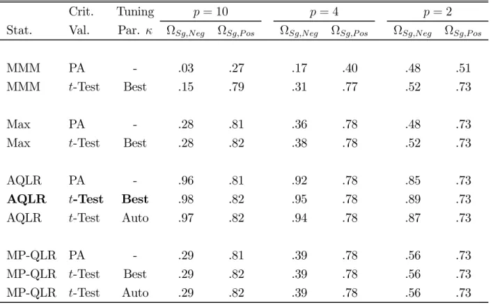
Similarly, the Max/PA and SumMax/PA tests have low power. The AQLR/PA test has better power than the other PA tests, but it is still very low compared to the AQLR/t -Test/ Best test.

Table II also shows that the MMM/t-Test/ Best test has equal asymptotic average power to the AQLR/t-Test/ Best test for Zero and only slightly lower power for P os: But, it has substantially lower power for N eg: For example, for p = 10; the compar-ison is :18 versus :55: The Max/t-Test/ Best test has noticeably lower average power than the AQLR/t-Test/ Best test for N eg; slightly lower power for Zero; and essen-tially equal power for P os: It is strongly dominated in terms of average power. The SumMax/t-Test/ Best test also is strongly dominated by the AQLR/t-Test/ Best test in terms of asymptotic average power. The power di¤erences between these two tests are especially large for N eg: For example, for p = 10 and N eg; their powers are :20 and :55;respectively.

Next we compare tests that use the AQLR test statistic but di¤erent critical values— due to the use of di¤erent functions ': The AQLR/'(2)_{/ Best test is essentially} dom-inated by the AQLR/t-Test/ Best, although the di¤erences are not large. The AQLR /'(3)_{/ Best test has noticeably lower asymptotic average power than the AQLR/t} -Test/ Best test for N eg; somewhat lower power for Zero; and equal power for P os: The di¤erences increase with p:

The AQLR/'(4)_{/ Best test has almost the same asymptotic average power as the} AQLR/t-Test/ Best test for Zero and P os and slightly lower power for N eg: This

18_{Size-correction here is done for the …xed known value of :It is not based on the least-favorable} matrix because the results are asymptotic and can be estimated consistently.

19_{The maximum null rejection probability calculations used in the size correction were calculated} using vectors that consist of00_sand10_{s:Then, additional calculations were carried out to determine}

whether the maximum over ₂Rp_+;1 is attained at such a vector in each case. No evidence was found to suggest otherwise. See Section 7 of the Supplemental Material for details.

is because the '(4) _{and '}(1) _{functions are similar. The AQLR/MMSC/ Best test and} AQLR/t-Test/ Best tests have quite similar power. Nevertheless, the AQLR/MMSC/ Best test is not the recommended test for reasons given below. We experimented with several smooth versions of the '(1) _{critical value function in conjunction with the} AQLR statistic. We were not able to …nd any that improved upon the asymptotic average power of the AQLR/t-Test/ Best test. Some were inferior. All such tests have substantial disadvantages relative to the AQLR/t-test in terms of the computational ease of determining suitable data-dependent and values.

In conclusion, we …nd that the best (S; ') choices in terms of asymptotic average power (based on =Best) are: AQLR/t-Test and AQLR/MMSC, followed closely by AQLR/'(2) and AQLR/'(4): Each of these tests out-performs the PA tests by a wide margin in terms of asymptotic power.

The AQLR/MMSC test has the following drawbacks: (i) its computation time is very high when p is large, such as p = 10; because the test statistic must be computed for all 2p _{possible combinations of selected moment vectors and (ii) the best value varies} widely with and p; which makes it quite di¢ cult to specify a data-dependent value that performs well. Similarly, the AQLR/'(2) _{and AQLR/'}(4) _{tests have substantial} computational drawbacks for determining a data-dependent values, see AJ2 for details. Based on the power results discussed above and on the computational factors, we take the AQLR/t-Test to be the recommended test and we develop data-dependent _b and bfor this test.

The last row of Table II gives the asymptotic power envelope, which is a “uni-directional”envelope, see AJ2 for details. One does not expect a test that is designed to perform well for multi-directional alternatives to be on, or close to, the uni-directional envelope. In fact, it is surprising how close the AQLR/t-Test/ Best test is to the power envelope when = P os:As expected, the larger ispthe greater is the di¤erence between the power of a test designed for p-directional alternatives and the uni-directional power envelope.

When the sample correlation matrix is singular, the QLR test statistic can be de…ned using the Moore-Penrose generalized inverse in the de…nition of the weighting matrix. Let MP-QLR denote this statistic. For the case of singular correlation matrices, AJ2 provides asymptotic power comparisons of the AQLR/t-Test/ Best test, the MP-QLR/t -Test/ Best test, and several other tests.

average power to that of the MP-QLR/t-Test/ Best test (e.g., .98 versus .29 when

p= 10) when the correlation matrix exhibits perfect negative correlation and the same power when only perfect positive correlation is present. Hence, it is clear that the adjustment made to the QLR statistic is bene…cial. The results also show that the AQLR/t-Test/ Best test strongly dominates tests based on the MMM and Max statistics in terms of asymptotic average power with singular correlation matrices.

Finally, results for the “pure ELR”test show that it has very poor asymptotic power properties.20 _{For example, forp= 10; its power ranges 1/3 to 1/7 that of the AQLR/t} -Test/ Best test (and of the feasible AQLR/t-Test/ Auto test, which is the recommended test of Section 2). The poor power properties of this “asymptotically optimal”test imply that the (generalized Neyman-Pearson) large deviations asymptotic optimality criterion is not a suitable criterion in this context.21

Note that the poor power of the “pure ELR” test does not imply that the ELR test statistic is a poor choice of test statistic. When combined with a good critical value, such as the data-dependent critical value recommended in this paper or a similar critical value, it yields a test with very good power. The point is that the large deviations asymptotic optimality result does not provide convincing evidence in favor of the ELR statistic.

5

Approximately Optimal

( )

and

( )

Functions

First, for p= 2 and given ₂( 1;1); where denotes the correlation that appears in ; we compute numerically the values of that maximize the asymptotic average (size-corrected) power of the nominal :05 AQLR/t-Test test over a …ne grid of 31 values. We do this for each in a …ne grid of 43 values. Because the power results

20_{The power of the pure ELR test and AQLR/t-Test/ Auto test, which is the recommended test of} Section 2, in the nine cases considered in Table II are: forp= 10;(.19, .55), (.17, .67), and (.12, .82); forp= 4; (.44, .59), (.42, .69), (.39, .78); and forp= 2; (.57, .65), (.55, .69), and (.54, .73). See Table S-XIII of AJ2.

21_{In our view, the large-deviation asymptotic optimality criterion is not appropriate when comparing} tests with substantially di¤erent asymptotic properties under non-large deviations. In particular, this criterion is questionable when the alternative hypothesis is multi-dimensional because it implies that a test can be “optimal”against alternatives in all directions, which is incompatible with the …nite sample and local asymptotic behavior of tests in most contexts.

are size-corrected, a by-product of determining the best value for each value is the size-correction value that yields asymptotically correct size for each :

Second, by a combination of intuition and the analysis of numerical results, we postulate that for p 3the optimal function ( ) is well approximated by a function that depends on only through the [ 1;1]-valued function ( ) de…ned in (2.9).

The explanation for this is as follows: (i) Given ; the value ( ) that yields maximum asymptotic average power is such that the size-correction value ( ) is not very large. (This is established numerically for a variety ofpand :) The reason is that the larger is ( );the larger is the fraction, ( )=(cn( ; ( )) + ( )) of the critical value that does not depend on the data (for known), the closer is the critical value to the PA critical value that does not depend on the data at all (for known ); and the lower is the power of the test for vectors that have less thanp elements negative and some elements strictly positive. (ii) The size-correction value ( ) is small if the rejection probability at the least-favorable null vector is close to when using the size-correction factor ( ) = 0: (This is self-evident.) (iii) We postulate that null vectors that have two elements equal to zero and the rest equal to in…nity are nearly least-favorable null vectors.22 _{If true, then the size of the AQLR/t-Test test depends on the} two-dimensional sub-matrices of that are the correlation matrices for the cases where only two moment conditions appear. (iv) The size of a test for given and p = 2 is decreasing in the correlation :In consequence, the least-favorable two-dimensional sub-matrix of is the one with the smallest correlation. Hence, the value of that makes the size of the test equal to for a small value of is (approximately) a function of through ( ) de…ned in (2.9). (Note that this is just a heuristic explanation. It is not intended to be a proof.)

Next, because ( )corresponds to a particular2 2submatrix of with correlation

(= ( ));we take ( )to be the value that maximizes asymptotic average power when

p = 2 and = ; as speci…ed in Table I and described in the second paragraph of this section. We take ( ) to be the value determined by p= 2 and ; i.e., 1( ) in (2.10) and Table I, but allow for an adjustment that depends onp;viz., 2(p);that is de…ned to guarantee that the test has correct asymptotic signi…cance level (up to numerical error).

22_{The reason for this postulation is that a test with given has larger null rejection probability the} more negative are the correlations between the moments. A variance matrix of dimension three by three or greater has restrictions on its correlations imposed by the positive semi-de…niteness property. If all of the correlations are equal, they cannot be arbitarily close to 1:In constrast, with a two-dimensional variance matrix, the correlation can be arbitarily close to 1:

See AJ2 for details.

We refer to the proposed method of selecting ( ) and ( ); described in Section 2, as the Auto method. We examine numerically how well the Auto method does in approximating the best ; viz., ( ):23 _{We provide four groups of results and consider}

p= 2;4;10 for each group. The …rst group consists of the three matrices considered in Table II. The rows of Table II for the AQLR/t-Test/ Best and AQLR/t-Test/ Auto tests show that the Auto method works very well. It has the same asymptotic average power as the AQLR/t-Test/ Best test for allp and values except one case where the di¤erence is just :01:

The second group consists of a set of 19 matrices for which ( ) takes values on a grid in [ :99; :99]: In 53 of the 57 (=3 19) cases, the di¤erence in asymptotic average power of the AQLR/t-Test/ Best and AQLR/t-Test/ Auto tests is less than :01:

The third group consists of two singular matrices. One with perfect negative and positive correlations and the other with perfect positive correlations. The AQLR/t -Test/ Auto test has the same asymptotic average power as the AQLR/t-Test/ Best test for 3 (p; )combinations, power that is lower by :01for 2 combinations, and power that is lower by :02for one combination.

The fourth group consists 500 randomly generated matrices for p= 2;4 and 250 randomly generated matrices for p = 10: For p = 2; across the 500 matrices, the asymptotic average power di¤erences have average equal to :0010; standard deviation equal to :0032; and range equal to [:000; :022]: For p = 4; across the 500 matrices, the average power di¤erence is :0012; the standard deviation is :0016; and the range is

[:000; :010]: For p = 10; across the 250 matrices, the average power di¤erences have average equal to:0183;standard deviation equal to:0069;and range equal to[:000; :037]:

In conclusion, the Auto method performs very well in terms of selecting values that maximize the asymptotic average power.

6

Finite-Sample Results

The recommended RMS test, AQLR/t-Test/ Auto, can be implemented in …nite samples via the “asymptotic normal” and the bootstrap versions of the t-Test/ Auto critical value. Here we determine which of these two methods performs better in …nite samples. We also compare these tests to the bootstrap version of the ELR/t-Test/ Auto

23_{For brevity, details of the numerical results are given in AJ2.}

test, which has the same …rst-order asymptotic properties as the AQLR-based tests (for correlation matrices whose determinants are bounded away from zero by " = :012 or more). See Sec. 6.3.3 of AJ2 for the de…nition of the ELR statistic and details of its computation.

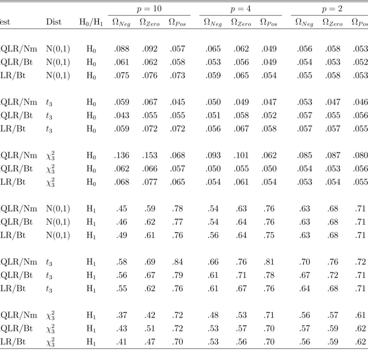
In short, we …nd that the bootstrap version (denoted Bt in Table III) of the AQLR/t -Test/ Auto test performs better than the asymptotic normal version (denoted Nm) in terms of the closeness of its null rejection probabilities to its nominal level and similarly on average in terms of its power. The AQLR bootstrap test also performs slightly better than the ELR bootstrap test in terms of power, is noticeably superior in terms of computation time, and is essentially the same (up to simulation error) in terms of null rejection probabilities. In addition, the AQLR bootstrap test is found to perform quite well in an absolute sense. Its null rejection probabilities are close to its nominal level and the di¤erence between its …nite-sample and asymptotic power is relatively small.

We provide results for sample size n = 100: We consider the same correlation matrices N eg; Zero; and P os as above and the same numbers of moment inequal-ities p = 2; 4; and 10: We take the mean zero variance Ip random vector Zy =

V ar 1=2_(m(W

i; ))(m(Wi; ) Em(Wi; )) to be i.i.d. across elements and consider three distributions for the elements: standard normal (i.e., N(0, 1)),t3;and chi-squared with three degrees of freedom 2

3: All of these distributions are centered and scaled to have mean zero and variance one. The power results are “size-corrected” based on the true matrix. For p = 2; 4; and 10; we use 5000, 3000, and 1000 critical value and rejection probability repetitions, respectively, for the results under the null and under the alternative.24

We note that the …nite-sample testing problem forany moment inequality model …ts into the framework above for some correlation matrix and some distribution of Zy_:

Hence, the …nite-sample results given here provide a level of generality that usually is lacking with …nite-sample simulation results.

The upper part of Table III provides the …nite-sample maximum null rejection prob-abilities (MNRP’s) of the nominal .05 normal and bootstrap versions of the AQLR/t -Test/ Auto test as well the bootstrap version of the ELR/t-Test/ Auto test. The MNRP is the maximum rejection probability over mean vectors in the null hypothesis for a given correlation matrix and a given distribution of Zy_{: The lower part of Table}

24_{The binding constraint on the number of simulation repetitions is the ELR test, see below for} details.

III provides MNRP-corrected …nite-sample average power for the same three tests. The average power results are for the same mean vectors in the alternative hypothesis as considered above for asymptotic power.

Table III shows that the AQLR/t-Test/ Auto bootstrap test performs well with MNRP’s in the range of[:043; :066]:In contrast, the AQLR normal test over-rejects some-what for some matrices with the normal and t3 distributions for which its MNRP’s are in the range of [:045; :092]: With the skewed distribution, 2

3; the AQLR normal test over-rejects the null hypothesis substantially with its MNRP’s being in the range

[:068; :153]:The fact that over-rejection is largest for a skewed distribution is not surpris-ing because the …rst term in the Edgeworth expansion of a sample average is a skewness term and the statistics considered here are simple functions of sample averages.

The ELR bootstrap test performs similarly to the AQLR bootstrap test in terms of null rejection probabilities. Its average amount of over-rejection over the 27 cases is

:012; whereas it is :005 for the AQLR bootstrap test. For the N(0, 1), t; and 2

3 distributions, Table III shows that the AQLR bootstrap test has …nite-sample average power compared to the AQLR normal test that is similar, inferior, and superior, respectively.

The ELR bootstrap test performs similarly to the AQLR bootstrap test in terms of power. Computation of the ELR/t-Test/ Auto bootstrap test usingR =10,000 simula-tion repetisimula-tions takes9:5;11:8;16:2;31:9;59:0;and182:7seconds whenp= 2;4;10;20;

30;and 50; respectively, andn= 250 using GAUSS on a PC with a 3.4 GHz processor. This is slower than the AQLR/t-Test/ Auto bootstrap test (see Section 2) by a factor of 4:4to 7:7:

AJ2 reports additional …nite-sample results for the case of singular correlation ma-trices. The results for the AQLR/t-Test/ Auto test show that the bootstrap version performs better than the normal version in terms of MNRP’s but similarly in terms of average power. Both tests perform well in an absolute sense. The bootstrap version of the MP-QLR/t-Test/ Auto test also is found to have good MNRP’s. However, its …nite-sample average power is much inferior to that of the AQLR/t-Test/ Auto boot-strap test— quite similar to the asymptotic power di¤erences.

For the ELR/t-Test/ Auto bootstrap test, results for singular correlation matrices are reported in AJ2 only for the case of p = 2: The reason is that with a singular correlation matrix, the Hessian of the empirical likelihood objective function is singu-lar a.s., which causes di¢ culties for standard derivative-based optimization algorithms

when computing the ELR test statistic. With p = 4 and p = 10; the constrained op-timization algorithm in GAUSS exhibits convergence problems and computation times are prohibitively large. For p= 2; the ELR bootstrap test’s performance is essentially the same as that of the AQLR bootstrap test in terms of MNRP’s and power.

In conclusion, we …nd that the AQLR/t-test/ Auto bootstrap test, which is the recommended test, performs well in an absolute sense with both nonsingular and singular variance matrices and out-performs the other tests considered in terms of asymptotic and …nite-sample MNRP’s or power, computational time, and/or computational stability.

References

Andrews, D. W. K. (1999): “Consistent Moment Selection Procedures for Generalized Method of Moments Estimation,”Econometrica, 67, 543–564.

Andrews, D. W. K. and P. Guggenberger (2009): “Validity of Subsampling and “Plug-in Asymptotic” Inference for Parameters De…ned by Moment Inequalities,” Econo-metric Theory, 25, 669-709.

Andrews, D. W. K. and P. Jia (2008): “Supplemental Material to ‘Inference for Pa-rameters De…ned by Moment Inequalities: A Recommended Moment Selection Procedure’,” unpublished manuscript, Cowles Foundation, Yale University.

Andrews, D. W. K. and G. Soares (2010): “Inference for Parameters De…ned by Mo-ment Inequalities Using Generalized MoMo-ment Selection,”Econometrica, 78, 119-157.

Bugni, F. A. (2010): “Bootstrap Inference in Partially Identi…ed Models De…ned by Moment Inequalities: Coverage of the Identi…ed Set,”Econometrica, 78, 735-753.

Canay, I. A. (2010): “EL Inference for Partially Identi…ed Models: Large Deviations Optimality and Bootstrap Validity,”Journal of Econometrics, 156, 408-425. Chernozhukov, V., H. Hong, and E. Tamer (2007): “Estimation and Con…dence Regions

for Parameter Sets in Econometric Models,”Econometrica, 75, 1243-1284.

Fan, Y. and S. Park (2007): “Con…dence Sets for Some Partially Identi…ed Parameters,” unpublished manuscript, Department of Economics, Vanderbilt University.

Imbens, G. and C. F. Manski (2004): “Con…dence Intervals for Partially Identi…ed Parameters,”Econometrica, 72, 1845-1857.

Pakes, A., J. Porter, K. Ho, and J. Ishii (2004): “Applications of Moment Inequalities,” unpublished working paper, Department of Economics, Harvard University.

Romano, J. P. and A. M. Shaikh (2008): “Inference for Identi…able Parameters in Par-tially Identi…ed Econometric Models,”Journal of Statistical Inference and Plan-ning (Special Issue in Honor of T. W. Anderson), 2786-2807.

Rosen, A. M. (2008): “Con…dence Sets for Partially Identi…ed Parameters That Satisfy a Finite Number of Moment Inequalities,”Journal of Econometrics,146, 107-117.

Table I. Moment Selection Tuning Parameters ( )and Size-Correction Factors 1( ) and 2(p) for =:051 ( ) ₁( ) ( ) ₁( ) ( ) ₁( ) [ 1; :975) 2:9 :025 [ :30; :25) 2:1 :111 [:45; :50) 0:8 :023 [ :975; :95) 2:9 :026 [ :25; :20) 2:1 :082 [:50; :55) 0:6 :033 [ :95; :90) 2:9 :021 [ :20; :15) 2:0 :083 [:55; :60) 0:6 :013 [ :90; :85) 2:8 :027 [ :15; :10) 2:0 :074 [:60; :65) 0:4 :016 [ :85; :80) 2:7 :062 [ :10; :05) 1:9 :082 [:65; :70) 0:4 :000 [ :80; :75) 2:6 :104 [ :05; :00) 1:8 :075 [:70; :75) 0:2 :003 [ :75; :70) 2:6 :103 [:00; :05) 1:5 :114 [:75; :80) 0:0 :002 [ :70; :65) 2:5 :131 [:05; :10) 1:4 :112 [:80; :85) 0:0 :000 [ :65; :60) 2:5 :122 [:10; :15) 1:4 :083 [:85; :90) 0:0 :000 [ :60; :55) 2:5 :113 [:15; :20) 1:3 :089 [:90; :95) 0:0 :000 [ :55; :50) 2:5 :104 [:20; :25) 1:3 :058 [:95; :975) 0:0 :000 [ :50; :45) 2:4 :124 [:25; :30) 1:2 :055 [:975; :99) 0:0 :000 [ :45; :40) 2:2 :158 [:30; :35) 1:1 :044 [:99;1:0] 0:0 :000 [ :40; :35) 2:2 :133 [:35; :40) 1:0 :040 [ :35; :30) 2:1 :138 [:40; :45) 0:8 :051 p 2 3 4 5 6 7 8 9 10 2(p) :00 :15 :17 :24 :31 :33 :37 :45 :50 1_{The values in Table I are obtained by simulating asymptotic formulae using 40,000} critical-value and 40,000 rejection-probability simulation repetitions, see AJ2 for details.

Table II. Asymptotic Average Power Comparisons (Size-Corrected): MMM, Max, SumMax, & AQLR Statistics, & PA, t-Test, '(2); '(3); '(4); & MMSC Critical Values with =Best1

Crit. Tuning p= 10 p= 4 p= 2

Stat. Val. Par. N eg Zero P os N eg Zero P os N eg Zero P os

MMM PA - .04 .36 .34 .20 .53 .45 .48 .62 .59

MMM t-Test Best .18 .67 .79 .31 .69 .76 .51 .69 .72

Max PA - .19 .44 .70 .30 .57 .71 .48 .64 .66

Max t-Test Best .25 .58 .82 .35 .66 .78 .51 .69 .72

SumMax PA - .10 .43 .62 .20 .55 .60 .48 .62 .59

SumMax t-Test Best .20 .65 .81 .31 .69 .77 .51 .69 .72

AQLR PA - .35 .36 .69 .46 .53 .70 .58 .69 .65

AQLR t-Test Best .55 .67 .82 .60 .69 .78 .65 .69 .73

AQLR t-Test Auto .55 .67 .82 .59 .69 .78 .65 .69 .73

AQLR '(2) _{Best .51}y _.65y _.81y _.60} _{.69 .78 .66 .69 .72}

AQLR '(3) _{Best .43}y _.63y _.81y _.55} _{.68 .78 .61 .69 .72}

AQLR '(4) _{Best .51}y _.65y _.81y _.60} _{.70 .78 .66 .69 .72}

AQLR MMSC Best .56y _.66y _.81y _{.63 .69 .78 .65 .69 .73}

Power Envelope - .85 .85 .85 .80 .80 .80 .75 .75 .75

1 _{=Best denotes the value that maximizes asymptotic average power. All cases} not marked with a ; }; or y are based on (40,000, 40,000, 40,000) critical-value, size-correction, and power repetitions, respectively.

Results are based on (5000, 5000, 5000) repetitions.

}_{Results are based on (2000, 2000, 2000) repetitions.} y_{Results are based on (1000, 1000, 1000) repetitions.}

Table III. Finite-Sample Maximum Null Rejection Probabilities (MNRP’s) and (“Size-Corrected”) Average Power of the Nominal .05 AQLR/t-Test/ Auto Test with Normal (AQLR/Nm) and Bootstrap-Based (AQLR/Bt) Critical Values and ELR/t-Test/ Auto Test with Bootstrap-Based (ELR/Bt) Critical Values

p= 10 p= 4 p= 2

Test Dist H0/H1 N eg Zero P os N eg Zero P os N eg Zero P os

AQLR/Nm N(0,1) H0 .088 .092 .057 .065 .062 .049 .056 .058 .053 AQLR/Bt N(0,1) H0 .061 .062 .058 .053 .056 .049 .054 .053 .052 ELR/Bt N(0,1) H0 .075 .076 .073 .059 .065 .054 .055 .058 .053 AQLR/Nm t3 H0 .059 .067 .045 .050 .049 .047 .053 .047 .046 AQLR/Bt t3 H0 .043 .055 .055 .051 .058 .052 .057 .055 .056 ELR/Bt t3 H0 .059 .072 .072 .056 .067 .058 .057 .057 .055 AQLR/Nm 2 3 H0 .136 .153 .068 .093 .101 .062 .085 .087 .080 AQLR/Bt 2 3 H0 .062 .066 .057 .050 .055 .050 .054 .053 .056 ELR/Bt 2 3 H0 .068 .077 .065 .054 .061 .054 .053 .054 .055 AQLR/Nm N(0,1) H1 .45 .59 .78 .54 .63 .76 .63 .68 .71 AQLR/Bt N(0,1) H1 .46 .62 .77 .54 .64 .76 .63 .68 .71 ELR/Bt N(0,1) H1 .49 .61 .76 .56 .64 .75 .63 .68 .71 AQLR/Nm t3 H1 .58 .69 .84 .66 .76 .81 .70 .76 .72 AQLR/Bt t3 H1 .56 .67 .79 .61 .71 .78 .67 .72 .71 ELR/Bt t3 H1 .55 .62 .76 .61 .67 .76 .64 .68 .71 AQLR/Nm 2 3 H1 .37 .42 .72 .48 .53 .71 .56 .57 .61 AQLR/Bt 23 H1 .43 .51 .72 .53 .57 .70 .57 .59 .62 ELR/Bt 23 H1 .41 .47 .70 .53 .56 .70 .56 .59 .62

Supplemental Material to

“Inference for Parameters De

fi

ned by

Moment Inequalities: A Recommended

Moment Selection Procedure”

Donald W. K. Andrews

Cowles Foundation for Research in Economics

Yale University

Panle Jia

Department of Economics

MIT

June 2008

Revised: May 2011

∗

_{Andrews gratefully acknowledges the research support of the National}

Science Foundation via grant SES-0751517. The authors thank Steve

Berry for numerous discussions and comments and the co-editor and

Contents

1 Introduction . . . 2 2 Moment Inequality/Equality Model . . . 4 3 Test Statistics . . . 5 4 Refined Moment Selection . . . 8 4.1 Basic Idea and Tuning Parameter κb . . . 9 4.2 Moment Selection Function ϕ . . . 10 4.3 RMS Critical Value cn(θ) . . . 12

4.4 Size-Correction Factor _bη . . . 13 4.5 Plug-in Asymptotic Critical Values . . . 15 5 Asymptotic Results . . . 16 5.1 Asymptotic Size . . . 16 5.2 Asymptotic Power . . . 17 5.3 Average Power . . . 20 5.4 Asymptotic Power Envelope . . . 22 6 Numerical Results . . . 22 6.1 Approximately Optimal κ(Ω) andη(Ω) Functions . . . 23 6.1.1 Definitions of κ(Ω) and η(Ω) . . . 23 6.1.2 Automaticκ Power Assessment . . . 25 6.2 AQLR Statistic and Choice of ε . . . 27 6.3 Singular Variance Matrices . . . 29 6.3.1 Asymptotic Power Comparisons . . . 29 6.3.2 Finite-Sample MNRP and Power Comparisons . . . 32 6.3.3 ELR Test with Singular Correlation Matrix . . . 35 6.4 κ Values That Maximize Asymptotic Average Power . . . 36 6.5 Comparison of(Sϕ)Functions: 19 ΩMatrices . . . 40 6.6 Comparison of RMS and GMS Procedures . . . 42 6.7 Additional Asymptotic MNRP & Power Results . . . 44 6.8 Comparative Computation Times . . . 49 6.9 Magnitude of RMS Critical Values . . . 49 7 Details Concerning the Numerical Results . . . 52 7.1 μVectors . . . 52 7.2 Automaticκ Power Assessment Details . . . 54

7.3 Asymptotic Power Envelope . . . 55 7.4 Computation ofκ Values That Maximize Asymptotic

Average Power . . . 55 7.5 Numerical Computation ofη₂(p) . . . 56 7.6 Maximization Over μVectors in the Null Hypothesis . . . 57 7.6.1 Computation ofη₂(p) . . . 57 7.6.2 Computation of MNRP’s for Tests Based on Best Kappa Values . 60 8 Computer Programs . . . 66 9 Alternative Parametrization and Proofs . . . 67 9.1 Alternative Parametrization . . . 68 9.2 Proofs . . . 70

1

Introduction

This paper contains Supplemental Material to the paper Andrews and Jia (2008), which we refer to hereafter as AJ1.

The contents of this paper are summarized as follows.

Sections 2-5 provide the asymptotic results upon which AJ1 is based.

Section 2 specifies the model considered, which allows for both moment inequalities and equalities (whereas AJ1 only considers moment inequalities).

Section 3 defines the class of test statistics that are considered.

Section 4 defines in detail the class of refined moment selection (RMS) critical values that are introduced in AJ1, gives the basic idea behind RMS critical values, defines data-dependent tuning parameters _b and data-dependent size-correction factors _b and discusses plug-in asymptotic (PA) critical values.

Section 5 establishes that RMS CS’s have correct asymptotic size (defined in a uni-form sense), derives the asymptotic power of RMS tests against local alternatives, dis-cusses an asymptotic average power criterion for comparing RMS tests, and disdis-cusses the uni-dimensional asymptotic power envelope.

Section 6 provides supplemental numerical results to those reported in AJ1. Sec-tion 6.1 contains addiSec-tional results that assess the performance of the data-dependent method for choosing_band_b for the AQLR/-Test/Auto test. Section 6.2 discusses the determination of the recommended adjustment constant =012 for the recommended AQLR test statistic. Section 6.3 considers the case where the sample moments have a

singular asymptotic correlation matrix. It provides comparisons of several tests based on their asymptotic average power, finite-sample maximum null rejection probabilities (MNRP’s), andfinite-sample average power. Section 6.4 provides tables of the values that maximize asymptotic average power (i.e., the best values), which are used in the construction of Table II of AJ1 and of the asymptotic MNRP’s (which are used for “size-correction”) of the RMS tests that appear in Table II of AJ1 (which reports asymptotic power) when no size-correction factor is employed, i.e.,  = 0 Section 6.5 is similar to Section 4 of AJ1, which compares the asymptotic power of various RMS tests, except that it considers 19 correlation matrices Ω (rather than three) but fewer tests. Section 6.6 compares several generalized moment selection (GMS) and RMS tests, where the GMS tests are based on non-data-dependent tuning parametersand no size-correction factors  Section 6.7 gives asymptotic MNRP and power results for some tests that are not considered in AJ1. Section 6.8 discusses the relative computation times of the asymptotic normal and bootstrap versions of the AQLR/-Test/Auto and MMM/ -Test/= 235tests. Section 6.9 provides information on the magnitude of the (random) RMS critical values for the recommended AQLR/-Test/Auto test.

Section 7 provides details concerning the numerical results reported in AJ1 and in Section 6 of this paper. Section 7.1 provides the  vectors used in AJ1 (which define the alternatives over which asymptotic and finite-sample average power is computed). Section 7.2 describes some details concerning the assessment of the properties of the automatic method of choosing Section 7.3 discusses the determination and computa-tion of the asymptotic power envelope. Seccomputa-tion 7.4 discusses the computacomputa-tion of the 

values that maximize asymptotic average power that are reported in Table II of AJ1. Sections 7.5 and 7.6 describe the numerical computation of ₂() which is part of the recommended size-correction function(_·)

Section 8 describes the GAUSS computer programs that were used to compute the numerical results.

Section 9 gives an alternative parametrization of the moment inequality/equality model to that given in AJ1 (that is conducive to the calculation of the uniform asymp-totic properties of CS’s and tests) and provides proofs of the results given in Section 5.

Throughout, we use the following notation. Let + = _{ _∈  :  _≥ 0_} ++ = { _∈  :   0_} +∞ = + ∪{+∞} [+∞] =  ∪{+∞} [±∞] =  ∪{±∞}  _=

×_× (with  copies) for any set  _∞ _{= (+}

All limits are as  _{→ ∞} unless specified otherwise. Let “df” abbreviate “distribution function,” “pd” abbreviate “positive definite,” (Ψ) denote the closure of a setΨand

0 denote a-vector of zeros.

2

Moment Inequality/Equality Model

For brevity, the model considered in AJ1 only allows for moment inequalities. Here we consider a more general model that allows for both inequalities and equalities. The moment inequality/equality model is as follows. The true value 0 (_∈ Θ _⊂ ) is assumed to satisfy the moment conditions:

0( 0) ≥ 0 for  = 1   and

0( 0) = 0 for  =+ 1  + (2.1)

where _{(· ) :  = 1  } are known real-valued moment functions,  =+ and

{ :  ≥ 1} are i.i.d. or stationary random vectors with joint distribution 0 Either

 or  may be zero. The observed sample is _{ :  ≤ } The true value 0 is not necessarily identified.

We are interested in tests and confidence sets (CS’s) for the true value 0

Generic values of the parameters are denoted ( ) For the case of i.i.d. observa-tions, the parameter space _F for( )is the set of all ( ) that satisfy:

(i) _∈Θ (ii)( )≥0 for  = 1   (iii) ( ) = 0 for =+ 1   (iv) _{:≥1} are i.i.d. under 

(v)2_() = (( ))0 (vi)(( ))∈Ψ and

(vii)|( )()|2+ ≤ for  = 1   (2.2) where (·)and(·)denote variance and correlation matrices, respectively, when

 is the true distribution,Ψis the parameter space for_×correlation matrices specified at the end of Section 3, and  _∞ and 0 are constants.

The asymptotic results apply to the case of dependent observations. We specify

F for dependent observations in Section 9 below. The asymptotic results also apply when the moment functions in (2.1) depend on a parameter i.e., when they are of the form _{(  ) :  ≤ } and a preliminary consistent and asymptotically normal

estimator b(0) of  exists (where 0 is the true value of ) The existence of such an estimator requires that  is identified given 0 In this case, the sample moment functions take the form () = (b()) (= −1P_=1( b())) The asymptotic variance of 12_

() typically is affected by the estimation of  and is defined accordingly. Nevertheless, all of the asymptotic results given below hold in this case using the definition of_F given in Section 9 below with the definitions of( ) and() changed suitably, as described there.

We consider a confidence set obtained by inverting a test. The test is based on a test statistic (0) for testing0 :=0 The nominal level1− CS for  is

 ={ ∈Θ:()≤()} (2.3) where () is a data-dependent critical value.1 In other words, the confidence set includes all parameter values  for which one does not reject the null hypothesis that 

is the true value.

3

Test Statistics

In this section, we define the test statistics () that we consider. The statistic

() is of the form () = (12()Σb()) where () = (1()  ())0 () =−1  X =1 ( ) for  ≤ (3.1) b

Σ()is a×variance matrix estimator defined below,is a real function on(_[+∞]×

₎

×V×andV×is the space of× variance matrices. (The set_[+∞]× contains

-vectors whose first  elements are either real or +_∞ and whose last  elements are real.)

The estimatorΣb()is an estimator of the asymptotic variance matrix of the sample

1_{Whenis in the interior of the identified set, it may be the case that}

() = 0 and() = 0In

moments 12() When the observations are i.i.d. and no parameter appears, b Σ() = −1  X =1 (( )−())(( )−())0 where ( ) = (1( )  ( ))0 (3.2) The correlation matrix Ωb()that corresponds to Σb()is defined by

b

Ω() =b−12()Σb()b−12() whereb() =(Σb()) (3.3) and(Σ) denotes the diagonal matrix based on the matrixΣ

With temporally dependent observations or when a preliminary estimator of a pa-rameter  appears, a different definition of Σb() often is required, see Section 9. For example, with dependent observations, a heteroskedasticity and autocorrelation consis-tent (HAC) estimator may be required.

We now define the leading examples of the test statistic function  Thefirst is the modified method of moments (MMM) test function 1 defined by

1(Σ) =  X =1 []2₋+ + X =+1 ()2 where []₋ = (  if  0 0 if _≥0  = (1  ) 0_{ (3.4)}

and2 is the th diagonal element of Σ AJ1 lists papers in the literature that consider this test statistic and the other test statistics below.2

The second function  is the quasi-likelihood ratio (QLR) test function 2 defined by

2(Σ) = inf

=(10):1∈+∞

(₋)0Σ−1(₋) (3.5) The origin of the QLR  function is as follows. Suppose one replaces  in (3.5) by a data vector _∈ _{that has a known}

× variance matrixΣThen, the resulting QLR statistic is the likelihood ratio statistic for the model with _∼(Σ) = (0

1 02)0 ∈ 

×  _{= }_{ the null hypothesis }∗

0 : 1 ≥ 0 & 2 = 0 and the alternative

2_{Several papers in the literature use a variant of}

1that is not invariant to rescaling of the moment

functions (i.e., with = 1for all)which is not desirable in terms of the power of the resulting test.