Classification in Networked Data: A Toolkit and a Univariate Case Study

Classification in Networked Data

:

A toolkit and a univariate case study

Sofus A. Macskassy [email protected]

Foster Provost [email protected]

New York University 44 W. 4th Street New York, NY 10012

Editor:

Abstract

This paper presents NetKit, a modular toolkit for classification in networked data, and a case-study of its application to a collection of networked data sets used in prior machine learning research. Networked data are relational data where entities are interconnected, and this paper considers the common case where entities whose labels are to be estimated are linked to entities for which the label is known. NetKit is based on a three-component framework, comprising a local classifier, a relational classifier, and a collective inference procedure. Various existing relational learning algo-rithms can be instantiated with appropriate choices for these three components and new relational learning algorithms can be composed by new combinations of components. The case study demon-strates how the toolkit facilitates comparison of different learning methods (which so far has been lacking in machine learning research). It also shows how the modular framework allows analysis of subcomponents, to assess which, whether, and when particular components contribute to supe-rior performance. The case study focuses on the simple but important special case of univariate network classification, for which the only information available is the structure of class linkage in the network (i.e., only links and some class labels are available). To our knowledge, no work pre-viously has evaluated systematically the power of class-linkage alone for classification in machine learning benchmark data sets. The results demonstrate clearly that simple network-classification models perform remarkably well—well enough that they should be used regularly as baseline clas-sifiers for studies of relational learning for networked data. The results also show that there are a small number of component combinations that excel, and that different components are preferable in different situations, for example when few versus many labels are known.

Keywords: relational learning, network learning, collective inference, collective classification, networked data

1. Introduction

This paper is about classification of entities in networked data, one type of relational data. Rela-tional classifier induction algorithms, and associated inference procedures, have been developed in a variety of different research fields and problem settings (Emde and Wettschereck, 1996; Flach and Lachiche, 1999; Dzeroski and Lavrac, 2001). Generally, these algorithms consider not only the features of the entities to be classified, but the relations to and the features of linked entities.

0. S.A. Macskassy and Provost, F.J., “Classification in Networked Data: A toolkit and a univariate case study” CeDER Working Paper CeDER-04-08, Stern School of Business, New York University, NY, NY 10012. December 2004.

Observed improvements in generalization performance demonstrate that taking advantage of rela-tional information in addition to attribute-value information can improve performance—sometimes substantially (e.g. (Taskar et al., 2001; Jensen et al., 2004)).

Networked data are the special case of relational data where entities are interconnected, such

as web-pages or research papers (connected through citations). This is in contrast with domains such as molecules or arches, where each entity is a self-contained graph and connections between the entities are absent or ignored. With a few exceptions (e.g., (Chakrabarti et al., 1998), (Taskar et al., 2001)), recent machine learning research on classification with networked data has focused on

across-network inference: learning from one network and applying the learned models to a separate,

presumably similar network (Craven et al., 1998; Lu and Getoor, 2003).

This paper focuses on within-network inference. In this case, networked data have the unique characteristic that training entities and entities whose labels are to be estimated are interconnected. Although the network may have disconnected components, generally there is not a clean separation between the entities for which class membership is known and the entities for which estimations of class membership are to be made. This introduces complications (Jensen and Neville, 2002b). For example, the usual careful separation of data into training and test sets is difficult. More important, thinking in terms of separating training and test sets obscures an important facet of the data: entities with known classifications can serve two roles. They act first as training data and subsequently as background knowledge during inference (Provost et al., 2003).

Many real-world problems, especially those involving social networks, exhibit opportunities for within-network classification. For example, in fraud detection entities to be classified as being fraudulent or legitimate are intertwined with those for which classifications are known. In coun-terterrorism and law enforcement, suspicious people may interact with known ‘bad’ people. Some networked data are by-products of social networks, rather than directly representing the networks themselves. For example, networks of web pages are built by people and organizations that are in-terconnected; when classifying web pages, some classifications (henceforth, labels) may be known and some may need to be estimated.

To our knowledge there has been no systematic study of machine learning methods for within-network classification that compares various algorithms on various data sets. A serious obstacle to undertaking such a study is the scarcity of available tools and source code, making it hard to compare various methodologies and algorithms. Such an in-depth study is further hindered by the fact that many relational learning algorithms can be separated into various sub-components. Ideally, a study should account for the contributions of the sub-components, and assess the relative advantage of alternatives. To enable such a study, we need a framework that facilitates isolating the performance of and interchanging sub-components.

As a main contribution of this paper, we introduce a network learning toolkit (NetKit-SRL) that enables in-depth, component-wise studies of techniques for statistical relational learning and inference with networked data. Starting with prior published work, we have abstracted the described algorithms and methodologies into a modular framework. The toolkit is based on this framework.1

NetKit is interesting for several reasons. First, it encompasses several currently available sys-tems, which are realized by choosing particular instantiations for the different components. This allows us to compare and contrast the different systems on equal footing. Perhaps more impor-tantly, the modularity of the toolkit broadens the design space of possible systems beyond those

that have appeared in prior published work, either by mixing and matching the components of the prior systems, or by introducing new alternatives for components. Finally, NetKit’s modularity not only allows allows for direct comparison of various models, but also for comparison of isolated components as we will show.

To illustrate, we use NetKit to conduct in an in-depth case study of within-network classifi-cation. The case study considers univariate learning and classification in homogeneous networks. We compare various techniques on twelve benchmark data sets from four domains used in prior machine learning research. Beyond illustrating the value of the toolkit, the case study makes sev-eral contributions. It provides systematic support for the claim that with networked data even uni-variate classification can be quite effective, and therefore it should be considered as a baseline against which to compare new relational learning algorithms (Macskassy and Provost, 2003). The case study illustrates a bias/variance tradeoff in networked classification, based on the principle of homophily (Blau, 1977; McPherson et al., 2001) (cf., assortativity (Newman, 2003) and auto-correlation (Jensen and Neville, 2002b). Indeed, the simplest method works so well it suggests that we should consider finding more diverse benchmark data sets. The case study also suggests network-classification analogues to feature selection and active learning.

The remainder of the paper is organized as follows. Section 2 describes the problem of net-work learning more formally, introduces the modular framenet-work, reviews prior net-work, and describes NetKit. Section 3 covers the case study, including the experimental methodology, data used, toolkit components used, and the results and analysis of the comparative study. The paper ends with dis-cussions of limitations and conclusions.

2. Network Learning

Traditionally, machine learning methods have treated entities as independent, which makes it possi-ble to infer class membership on an entity-by-entity basis. With networked data, the class member-ship of one entity may have an influence on the class membermember-ship of a related entity. Furthermore, entities not directly linked may be related by chains of links, which suggests that it may be beneficial to infer the class memberships of all entities simultaneously. Collective inferencing in relational data (Taskar et al., 2002; Neville and Jensen, 2004) makes simultaneous statistical judgments regarding the values of an attribute or attributes for multiple entities in a graphGfor which some attribute values are not known.

For the univariate case study presented below, the (single) attribute of vertexvi, representing the class, can take on some categorical valueX∈ X.

Given graph G = (V, E), a single attribute xi for each vertex vi ∈ V, and given known values forxi for some subset of verticesVK_{, univariate collective inferencing}

is the process of simultaneously inferring the values ofxi for the remaining vertices,

VU _=V−VK_{, or a probability distribution over those values.}

As a shorthand, we will usexK _{to denote the set (vector) of class values forV}K_{, and similarly} for xU_{. Then, G}K _{= (V, E,}xK_{) denotes everything that is known about the graph (we do not} consider the possibility of unknown edges). Edge eij ∈ E represents the edge between vertices vi andvj, andwij represents the edge weight. For this paper we consider only undirected edges, simply ignoring directionality if necessary for a particular application.

Rather than estimating the full joint probability distributionP(xU_|GK_{), relational learning} of-ten enhances tractability by making a Markov assumption:

P(xi|G) =P(xi|Ni), (1)

whereNi is the set of “neighbors” of vertexvi such thatP(xi|Ni)is independent ofG− Ni(i.e., P(xi|Ni) = P(xi|G)). For this paper, we make the (“first-order”) assumption thatNi comprises

only the immediate neighbors ofvi in the graph. As one would expect, and as we will see, this assumption can be violated to a greater or lesser degree based on how edges are defined.

GivenNi, a relational model can be used to estimatexi. Note thatNiU (=Ni∩VU)—the set

of neighbors ofviwhose values of attributexare not known—could be non-empty. Therefore, even if the Markov assumption holds, a simple application of the relational model may be insufficient. However, the relational model may be used to estimate the labels of NK

i = Ni −NiU. Further,

just as estimates for the labels ofNU

i influence the estimate forxi,xi also influences the estimate

of the labels ofNU

i . In order to simultaneously estimatexU, various collective methods have been

introduced for relational inference, including Gibbs sampling (Geman and Geman, 1984), loopy belief propagation (Pearl, 1988), relaxation labeling (Chakrabarti et al., 1998), and other iterative classification methods (Neville and Jensen, 2000; Lu and Getoor, 2003). All such methods require initial (“prior”) estimates of the values for P(xU_|GK_{). The priors could be Bayesian subjective} priors (Savage, 1954), or they could be estimated from data. A common estimation method is to employ a non-relational learner, using available “local” attributes ofvi to estimatexi(e.g., as done by Chakrabarti et al. (1998)). In the univariate case, such local attributes are not available; for our case study, we use the marginal class distribution overVKas the prior for allxi ∈xU_.

2.1 Network Learning Framework

As suggested by the discussion above, one prominent class of systems for learning and inference in networked data can be characterized by three main components. For each component, there are many possible instantiations.

1. Non-relational (“local”) model. This component consists of a (learned) model, which uses only local information—namely information about (attributes of) the entities whose target variable is to be estimated. The local models can be used to generate priors that comprise the initial state for the relational learning and collective inference components. They also can be used as one source of evidence during collective inference. These models typically are produced by traditional machine learning methods.

2. Relational model. In contrast to the non-relational component, the relational model makes use of the relations in the network as well as the values of attributes of related entities, pos-sibly through long chains of relations. Relational models also may use local attributes of the entities.

3. Collective inferencing. The collective inferencing component determines how the unknown values are estimated together, possibly influencing each other, as described above.

Certain techniques from prior work, described below, can be instantiated with particular choices of these components. For example, using a naive Bayes classifier as the local model, a naive Bayes

Markov Random Field classifier for the relational model, and relaxation labeling for the inferencing method forms the system used by Chakrabarti et al. (1998). Using logistic regression for the local and relational models, and iterative classification for the inferencing method produces Lu & Getoor’s (2003) link-based classifier. Using class priors for the local model, a (weighted) majority vote of neighboring classes for the relational model, and relaxation labeling for the inference method forms Macskassy & Provost’s (2003) relational neighbor classifier.

2.2 Prior Work

For machine learning research on networked data, the watershed paper of Chakrabarti et al. (1998) studied classifying web-pages based on the text and (possibly inferred) class labels of neighboring pages, using relaxation labeling paired with naive Bayes local and relational classifiers. In their experiments, using the link structure substantially improved classification over using the local (text) information alone. Further, considering the text of the neighbors generally hurt performance (based on the methods they used), whereas using only the (inferred) class labels improved performance.

More recently, Lu and Getoor (2003) investigated network classification applied to linked doc-uments (web pages and published manuscripts with an accompanying citation graph). Similarly to the work of Chakrabarti et al. (1998), Lu and Getoor (2003) use the text of the document as well as a relational classifier. Their “link-based” classifier was a logistic regression model based on a vector of aggregations of properties of neighboring nodes linked with different types of links (in-, out-, co-links). Various aggregates were considered, such as the mode (the value of the most often occurring neighbor class), a binary vector with a value of 1 at celliif there was a neighbor whose class label wasci, and a count vector where cellicontained the number of neighbors belonging to classci. In their experiments, the count model performed best.

Univariate within-network classification has been considered previously (Bernstein et al., 2002, 2003; Macskassy and Provost, 2003). Using business news, Bernstein et al. (2003) linked companies if they co-occurred in a news story. They demonstrated the effectiveness of various vector-space techniques for network classification of companies into industry sectors, based on vectors of class labels of the neighbors. This work did not use collective inferencing, performing only a one-shot prediction based on the known neighborhood (knowing90%of the class labels and predicting the remaining 10%). Other domains such as web-pages, movies and citation graphs have also been considered for univariate within-network classification; Macskassy and Provost (2003) investigated how well the univariate classification performed as varying amounts of data initially were labeled. They used a relaxation labeling method similar to that used by Chakrabarti et al. (1998). In both studies, a very simple model predicting class membership based on the most prevalent class in the neighborhood was shown to perform remarkably well. The present paper can be seen in part as a systematic followup to these workshop papers.

Markov Random Fields (MRFs) have been used extensively for univariate network classification for vision and image restoration. Nodes in the network are pixels in an image and the labels are image-related such as whether a pixel is part of a vertical or horizontal border (Dobrushin, 1968; Geman and Geman, 1984; Winkler, 2003). MRFs are used to estimate the joint probability of a set of nodes based on their immediate neighborhoods under the first-order Markov assumption that

P(xi|X/xi) = P(x|Ni), whereX/xi means all nodes inXexceptxi andNi is a neighborhood

function returning the neighbors ofvi. Chakrabarti et al. (1998) use an MRF formulation for their network classifier (described above), which we reconstruct in NetKit.

One popular method to compute the MRF joint probability is Gibbs sampling (described below). The most common use of Gibbs sampling in vision is not to compute the final posteriors as we do in this paper, but rather to get final classifications. One way to enforce that the Gibbs sampler settles to a final state is by using a simulated annealing approach where the temperature is dropped slowly until nodes no longer change state (Geman and Geman, 1984). Neville and Jensen (2000) used a simulated annealing approach in their iterative classification collective inference procedure, where a label for a given node was kept only if the relational classifier was confident about the label at a given threshold, otherwise the label would be set tonull. By slowly lowering this threshold, the system was eventually able to label all nodes. NetKit incorporates iterative classification based on the subsequent work of Lu and Getoor (2003) (described above).

Graph-cut techniques recently have been used in vision research as an alternative to using Gibbs sampling (Boykov et al., 2001), iteratively changing the labelings of many nodes at once by solving a min-cut/max-flow problem based on the current labelings. In addition to the explicit links in the data, each node is also connected to one special node per class label. A min-cut algorithm is then used to partition the graph such that only one class-node remains linked to each node in the data. Based on this cut, the method then changes the labelings, and repeats until no pixels change labels. These methods are very fast. NetKit does not yet incorporate graph-cut techniques.

Several recent methods apply to learning in networked data, beyond the homogeneous, univari-ate case treunivari-ated in this paper. Conditional Random Fields (CRFs) (Lafferty et al., 2001) are an extension of MRFs where labels are conditioned not only on the labels of neighbors, but also on the attributes of the node itself and the attributes of the neighborhood nodes. CRFs were applied to part-of-speech (POS) tagging in text, where the nodes in the graphs represented the words in the sentence, connected by their word order. The labels to be predicted were POS-tags and the attribute of a node was the word it represents. The neighborhood of a word comprised the words on either side of it.

Relational Bayesian Networks (RBNs)2(Koller and Pfeffer, 1998; Friedman et al., 1999; Taskar et al., 2001) extend Bayesian networks (BNs (Pearl, 1988)) by taking advantage of the fact that a variable used in one instantiation of a BN may refer to the exact same variable in another BN. For example, if the grade of a student depends upon his professor, this professor is the same for all students in the class. Therefore, rather than building one BN and using it in isolation for each entity, RBNs directly link shared variables in “unrolled” BNs, thereby generating one big network of connected entities for which collective inferencing can be performed. Most relevant to this paper, for within-network classification RBNs were applied by Taskar et al. (2001) to various domains, including a data set of published manuscripts linked by authors and citations. Loopy Belief Prop-agation (Pearl, 1988) was used to perform the collective inferencing. The study showed that the PRM performed better than a non-relational naive Bayes classifier and that using both author and citation information in conjunction with the text of the paper worked better than using only author or citation information in conjunction with the text.

Relational Dependency Networks (RDNs) (Neville and Jensen, 2003, 2004), extend dependency networks (Heckerman et al., 2000) in much the same way that RBNs extend Bayes Networks. RDNs have been used successfully on a bibliometrics data set, a movie data set and a linked web-page data set, where they were shown to perform much better than a relational probability tree (RPT)

2. These originally were called Probabilistic Relational Models (PRMs). PRM now typically is used as a more gen-eral term which includes other models such as Relational Dependency Networks and Relational Markov Networks, described next.

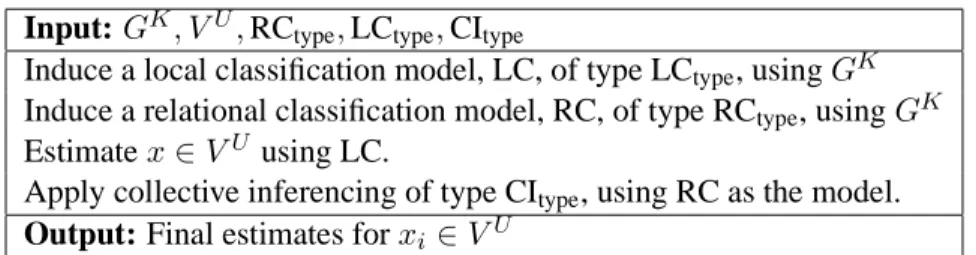
Input:GK_{, V}U_,RC

type,LCtype,CItype

Induce a local classification model, LC, of type LCtype, usingGK

Induce a relational classification model, RC, of type RCtype, usingGK

Estimatex∈VU_{using LC.}

Apply collective inferencing of type CItype, using RC as the model. Output: Final estimates forxi ∈VU

Table 1: High-level pseudo code for the main core of the Network Learning Toolkit.

(Neville et al., 2003) using no collective inferencing. Gibbs sampling was used to perform collective inferencing.

Relational Markov Networks (RMNs) (Taskar et al., 2002) extend Markov Networks (Pearl, 1988). The clique potential functions used are based on functional templates, each of which is a (learned, class-conditional) probability function based on a user-specified set of relations. Taskar et al. (2002) applied RMNs to a set of web-pages and showed that they performed better than other non-relational learners as well as naive Bayes and logistic regression when used with the same relations as the RMN. Loopy Belief Propagation was used to perform collective inferencing.

The above systems use only a few of the many relational learning techniques proposed in the lit-erature. There are many more, for example from the rich literature of inductive logic programming (ILP) (e.g. Flach and Lachiche (1999); Raedt et al. (2001); Dzeroski and Lavrac (2001); Kramer et al. (2001); Domingos and Richardson (2004)), or based on using relational database joins to gen-erate relational features (e.g. Perlich and Provost (2003); Popescul and Ungar (2003); Perlich and Provost (2004)). These techniques could be the basis for additional relational model components in NetKit.

2.3 Network Learning Toolkit (NetKit-SRL)

NetKit is designed to accommodate the interchange of components and the introduction of new components. Any local model can be paired with any relational model, which can then be combined with any collective inference method. NetKit’s core routine is simple and is outlined in Table 1.

NetKit consists of these primary modules:

1. Input: This module reads data into a memory-resident graphG.

2. Local classifier inducer (LC): Given as training dataVK_{, this module returns a model which}

using only attributes of a nodevi ∈ VU will estimatexi. Ideally, LC will estimate a

proba-bility distribution over the possible values forxi.

3. Relational classifier inducer (RC): GivenGK_{, this module returns a model which usingv} i

andNiwill estimatexi. Ideally, RC will estimate a probability distribution over the possible

values forxi.

4. Collective Inferencing: Given a graphGpossibly with somexiknown, a set of priors over xU_{, and a relational modelMR, this applies collective inferencing to estimate}xU_.

5. Weka Wrapper: This module is a wrapper for Weka3 (Witten and Frank, 2000) and will convert the graph representation ofviinto an entity that can either be learned from or be used to estimatexi.

Implementation details on these modules can be found in Appendix B. The current version of NetKit-SRL, while able to read in heterogeneous graphs, only supports classification in graphs consisting of a single type of node.

2.4 NetKit Components

This section describes the particular relational classifiers and collective inference methods imple-mented in NetKit for the univariate case study. First, we describe the four (univariate4) relational classifiers (RC components). Then, we describe the three collective inference methods.

2.4.1 RELATIONALCLASSIFIERS(RC)

All four relational classifiers take advantage of a first-order Markov assumption on the network: only a node’s local neighborhood is necessary for classification. The univariate case renders this assumption particularly restrictive: only the class labels of the local neighbors are necessary. The local network is defined by the user, analogous to the user’s definition of the feature set for proposi-tional learning. Entities whose class labels are not known are either ignored or are assigned a prior, depending upon the choice of local classifier.

2.4.1.1 WEIGHTED-VOTERELATIONALNEIGHBORCLASSIFIER(WVRN)

Our first and simplest classifier (cf., Macskassy and Provost (2003)5) estimates class-membership probabilities based on one assumption in addition to the Markov assumption: the entities exhibit homophily—i.e., linked entities have a propensity to belong to the same class (Blau, 1977; McPher-son et al., 2001). This homophily-based model is motivated by observations and theories of social networks (Blau, 1977; McPherson et al., 2001), where homophily is ubiquitous. Homophily was one of the first characteristics noted by early social network researchers (Almack, 1922; Bott, 1928; Richardson, 1940; Loomis, 1946; Lazarsfeld and Merton, 1954), and holds for a wide variety of different relationships (McPherson et al., 2001). It seems reasonable to conjecture that homophily may also be present in other sorts of networks, especially networks of artifacts created by people. (Recently assortativity, a link-centric notion of homophily, has become the focus of mathematical studies of network structure (Newman, 2003).)

Definition. Givenvi ∈VU, the weighted-vote relational-neighbor classifier (wvRN) estimates

P(xi|Ni)as the (weighted) mean of the class-membership probabilities of the entities inNi: P(xi=X|Ni) = 1 Z X vj∈Ni wi,j·P(xj =X|Nj), (2)

where Z is the usual normalizer. As the above is a recursive definition (for undirected graphs,

vj ∈ Ni ⇔ vi ∈ Nj) the classifier uses the “current” estimate for P(xj = X|Nj), where the

“current” estimate is defined by the collective inference technique being used.

3. We use version 3.4.2. Weka is available athttp://www.cs.waikato.ac.nz/˜ml/weka/ 4. The open-source NetKit release contains multivariate versions of these classifiers.

2.4.1.2 CLASS-DISTRIBUTIONRELATIONALNEIGHBORCLASSIFIER(CDRN)

Learning a model of the distribution of neighbor class labels may lead to better discrimination than simply using the (weighted) mode. Following Perlich and Provost (2003), and in the spirit of Rocchio’s method (Rocchio, 1971), we define nodevi’s class vectorCV(vi)to be the vector of

summed linkage weights to the various (known) classes, and classX’s reference vectorRV(X)to be the average of the class vectors for nodes known to be of classX. Specifically:

CV(vi)k=

X

vj∈Ni,xj=Xk

wi,j, (3)

whereCV(vi)k represents thekth position in the class vector andXk is thekth class. Based on

these class vectors, the reference vectors can then be defined as the vector sum:

RV(X) = 1 |VK X | X vi∈VXK CV(vi), (4) whereV_XK ={vi|vi ∈VK, xi =X}.

During training, neighbors in VU _{are ignored. For prediction, estimated class membership}

probabilities are used for neighbors inVU_{, and equation (3) becomes:} CV(vi)k=

X

vj∈Ni

P(xj =Xk|Nj)·wi,j (5)

Definition. Given vi ∈ VU, the class-distribution relational-neighbor classifier (cdRN)

es-timates the probability of class membership, P(xi = X|Ni), by the normalized vector distance

betweenvi’s class vector and classX’s reference vector:

P(xi =X|Ni) = 1

Zdist(CV(vi),RV(X)), (6)

whereZis the usual normalizer anddist(a, b)is any vector distance function (L1,L2, cosine, etc.). For the results presented below, we use cosine distance.

As with wvRN, Equation 5 is a recursive definition, and therefore the value ofP(xj =X|Nj)

is approximated by the “current” estimate as given by the selected collective inference technique. 2.4.1.3 NETWORK-ONLYBAYESCLASSIFIER(NBC)

NetKit’s network-only Bayes classifier (nBC) is based on the algorithm described by Chakrabarti et al. (1998). To start, assume there is a single nodevi inVU. The nBC uses multinomial naive Bayesian classification based on the classes ofvi’s neighbors.

P(xi =X|Ni) = P(Ni|X)·P(X) P(Ni) , (7) where P(Ni|X) = 1 Z Y vj∈Ni P(xj =Xj∗|xi =X)wi,j (8)

whereZ is a normalizing constant andXj∗is the class observed at nodev_j. BecauseP(N_i)is the

same for each class, normalization across the classes allows us to ignore it (as with naive Bayes generally).

We call nBC “network-only” to emphasize that in the application to the univariate case study be-low, we do not use local attributes of a node. As discussed above, Chakrabarti et al. initialize nodes’ priors based on a naive Bayes model over the local document text.6 In the univariate setting, local text is not available. We therefore use the same scheme as for the other RCs: initialize unknown labels as decided by the local classifier being used (either the class prior or ’null’, depending on the CI component, as described below). If a neighbor’s label is ’null’, then it is ignored for clas-sification. Also, Chakrabarti et al. differentiated between incoming and outgoing links, whereas we do not. Finally, Chakrabarti et al. do not mention how or whether they account for possible zeros in the estimations of the marginal conditional probabilities; we apply traditional Laplace smoothing wherem=|X |, the number of classes.

The foregoing assumes all neighbor labels are known. When the values of some neighbors are unknown, but estimations are available, we follow Chakrabarti et al. (1998) and perform Markov Random Fields (MRF) estimations (Dobrushin, 1968; Geman and Geman, 1984; Winkler, 2003), based on how different configurations of neighbors’ classes affect a target entity’s class. Specifically, the classifier computes a Bayesian combination based on (estimated) configuration priors and the entity’s known neighbors. Chakrabarti et al. (1998) describe this procedure in detail. For our case study, such an estimation is necessary only when using relaxation labeling (described below). 2.4.1.4 NETWORK-ONLYLINK-BASEDCLASSIFICATION(NLB)

The final relational classifier used in the case study is a network-only derivative of the link-based classifier (Lu and Getoor, 2003). The network-only Link-Based classifier (nLB) creates a feature vector for a node by aggregating the labels of neighboring nodes, and then uses logistic regression to build a discriminative model based on these feature vectors. This learned model is then applied to estimateP(xi=X|Ni). As with the nBC, the difference between the “network-only” link-based

classifier and Lu and Getoor’s version is that for the univariate case study we do not consider local attributes (e.g., text).

As described above, Lu and Getoor (2003) considered various aggregation methods: existence (binary), the mode, and value counts. The last aggregation method, the count model, is equivalent to the class vectorCV(vi)defined in Equation 5. This was the best performing method in the study

by Lu and Getoor, and is the method on which we base nLB. The logistic regression classifier used by nLB is the multiclass implementation from Weka version 3.4.2.

We made one minor modification to the original link-based classifier. Perlich (2003) argues that in different situations it may be preferable to use vectors based on raw counts (as given above) or vectors based on normalized counts. We did preliminary runs using both. The normalized vectors generally performed better, and so we use them for the case study.

2.4.2 COLLECTIVEINFERENCEMETHODS(CI)

This section describes three collective inferencing (CI) methods implemented in NetKit and used in the case study. As described above, given (i) a network initialized by the local model, and (ii) a relational model, a CI method infers a set of class labels forxU_{, ideally with the maximum joint} probability. Alternatively, if estimates of entities’ class-membership probabilities are needed, the

6. The original classifier was defined as:P₍x_i=X_{|Ni) =}P_(Ni|X_)·P₍τ_i|v_i)·P₍X_{), with}τ_{ibeing the text of the} document-entity represented by vertexv_i.

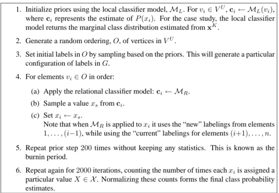
1. Initialize priors using the local classifier model,ML. Forvi ∈V U

,ci← ML(vi), whereci represents the estimate ofP(xi). For the case study, the local classifier model returns the marginal class distribution estimated fromxK

. 2. Generate a random ordering,O, of vertices inVU

.

3. Set initial labels inOby sampling based on the priors. This will generate a particular configuration of labels inG.

4. For elementsvi∈Oin order:

(a) Apply the relational classifier model:ci← MR. (b) Sample a valuexsfromci.

(c) Setxi←xs.

Note that whenMRis applied toxiit uses the “new” labelings from elements 1, . . . ,(i−1), while using the “current” labelings for elements(i+1), . . . , n. 5. Repeat prior step200 times without keeping any statistics. This is known as the

burnin period.

6. Repeat again for2000iterations, counting the number of times eachxiis assigned a particular valueX ∈ X. Normalizing these counts forms the final class probability estimates.

Table 2: Pseudo-code for Gibbs sampling.

CI method estimates the marginal probability distributionP(xi|GK_{,Λ)for eachxi∈x}U_{, whereΛ}

stands for the priors returned by the local classifier. 2.4.2.1 GIBBSSAMPLING(GS)

Gibbs sampling (GS) (Geman and Geman, 1984) is commonly used for collective inferencing with relational learning systems. The algorithm is straightforward and is shown in Table 2.7 The use of

200and2000for the burnin period and number of iterations are commonly used values.8 Ideally, we would iterate until the estimations converge. Although there are convergence tests for the Gibbs sampler, they are not robust nor well understood (cf. Gilks et al. (1995)), so we simply use a fixed number of iterations.

Notably, because all nodes are assigned a class at every iteration, when GS is used the relational models will always see a fully labeled/classified neighborhood, making prediction straightforward. For example, nBC does not need its MRF estimation.

2.4.2.2 RELAXATIONLABELING (RL)

The second collective inferencing method implemented and used in this study is relaxation labeling (RL), based on the method of Chakrabarti et al. (1998). Rather than treatG as being in a specific labeling “state” at every point (as Gibbs sampling does), relaxation labeling retains the uncertainty, keeping track of the current probability estimations forxU_{. The relational model must}

7. This instance of Gibbs sampling uses a single random ordering (“chain”), as this is what we used in the case study. In the case study, using10chains (the default in NetKit) had no effect on the final accuracies.

8. As it turns out, in our case study GS invariably reached a seemingly final plateau in fewer than1000iterations, and often in fewer than500.

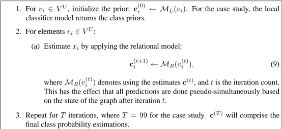
1. Forvi ∈ V U

, initialize the prior: c(0)_i ← ML(vi). For the case study, the local classifier model returns the class priors.

2. For elementsvi∈V U

:

(a) Estimatexiby applying the relational model: c(_it+1)_{← M}R(v(

t₎

i ), (9)

whereMR(v(it))denotes using the estimatesc(

t)_{, andtis the iteration count.} This has the effect that all predictions are done pseudo-simultaneously based on the state of the graph after iterationt.

3. Repeat forT iterations, whereT = 99for the case study. c(T)_{will comprise the} final class probability estimations.

Table 3: Pseudo-code for Relaxation Labeling.

be able to use these estimations. Further, rather than estimating one node at a time and updating the graph right away, relaxation labeling “freezes” the current estimations so that at stept+ 1, all vertices will be updated based on the estimations from stept. The algorithm is shown in Table 3.

Preliminary runs showed that RL sometimes does not converge, but rather ends up oscillating between two points.9 NetKit performs simulated annealing—on each subsequent iteration giving more weight to a node’s own current estimate and less to the influence of its neighbors.

The new updating step, replacing Equation 9, is defined as: c(t+1) i =β( t+1)_{· M} R(vi(t)) + (1−β( t+1)_)·c(t) i , (10) where β0 = k β(t+1) = β(t)·α, (11)

where kis a constant, which for the case study we set to 1.0, and α is a decay constant, which we set to0.99. Preliminary testing showed that final performance is very robust as long as0.9 < α < 1. Smaller values ofα can lead to neighbors losing their weight too quickly, which can hurt performance when only very few labels are known. A post-mortem of the results showed that the accuracies often converged within the first20iterations.

2.4.2.3 ITERATIVECLASSIFICATION(IC)

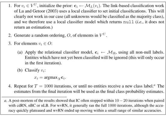
The third and final collective inferencing method implemented in NetKit and used in the case study is the variant of Iterative Classification described in the work on link-based classification (Lu and Getoor, 2003) and shown in Table 4. As with Gibbs sampling, the relational model never sees uncertainty in the labels of (neighbor) entities. Either the label of a neighbor isnulland ignored (which only happens in the first iteration), or it is assigned a definite label.

1. Forvi∈V U

, initialize the prior:ci← ML(vi). The link-based classification work of Lu and Getoor (2003) uses a local classifier to set initial classifications. This will clearly not work in our case (all unknowns would be classified as the majority class), and we therefore use a local classifier model which returnsnull(i.e., it does not return an estimation.)

2. Generate a random ordering,O, of elements inVU . 3. For elementsvi∈O:

(a) Apply the relational classifier model, ci ← MR, using all non-null labels. Entities which have not yet been classified will be ignored (this will only occur in the first iteration).

(b) Classifyvi:

xi=argmaxXci.

4. Repeat forT = 1000iterations, or until no entities receive a new class label.a _The estimates from the final iteration will be used as the final class probability estimates.

a. A post-mortem of the results showed that IC often stopped within10−20iterations when paired with cdRN, nBC or nLB. For wvRN, it generally ran the full1000iterations, although the accu-racy quickly plateaued and wvRN ended up moving within a small range of similar accuracies.

Table 4: Pseudo-code for Iterative Classification.

3. Case Study

The study presented in this section has two goals. First, it showcases NetKit, demonstrating that the modular framework indeed facilitates the comparison of systems for learning and inference in networked data. Second, it examines the simple-but-important special case of univariate learning and inference in homogeneous networks, comparing alternative techniques that have not before been compared systematically, if at all. The setting for the case study is simple: For some entities in the network, the value ofxiis known; for others it must be estimated.

Univariate classification, albeit a simplification for many domains, is important for several rea-sons. First, it is a representation that is used in some applications. In the introduction we mentioned fraud detection. As a specific example, a telephone account that calls the same numbers as a known fraudulent account (and hence the accounts are connected through these intermediary numbers) is suspicious (Fawcett and Provost, 1997; Cortes et al., 2001). For phone fraud, univariate network classification often provides alarms with reasonable coverage and remarkably low false-positive rates. In fact, the fraud detection work of Cortes et al. focuses on exactly this representation (albeit also considering changes in the network over time). Generally speaking, a homogeneous, univariate network is an inexpensive (in terms of data gathering, processing, storage) approximation of many complex networked data problems. Fraud detection applications certainly do have a variety of addi-tional attributes of importance; nevertheless, univariate simplifications are very useful and are used in practice.

The univariate case also is important scientifically. It isolates a primary difference between networked data and non-networked data, facilitating the analysis and comparison of relevant clas-sification and learning methods. One thesis of this study is that there is considerable information

Category Size High-revenue 572 Low-revenue 597

Total 1169

Base accuracy 51.07%

Table 5: Details on class distribution for the IMDb data set.

inherent in the structure of the networked data and that this information can be readily taken advan-tage of, using simple models, to estimate the labels of unknown entities. This thesis is tested by isolating this characteristic—namely ignoring any auxiliary attributes and only allowing the use of known class labels—and empirically evaluating how well univariate models perform in this setting on benchmark data sets.

Considering homogeneous networks plays a similar role. Although the domains we consider have obvious representations consisting of multiple entity types and edges (e.g., people and papers for node types and same-author-as and cited-by as edge types in a citation-graph domain), a homo-geneous representation is much simpler. In order to assess whether a more complex representation is worthwhile, it is necessary to assess standard techniques on the simpler representation (as we do in this case study). Of course, the way a network is “homogenized” may have a considerable effect on classification performance. We will revisit this below in Section 3.3.6.

3.1 Data

The case study reported in this paper makes use of 12 benchmark data sets from four domains that have been the subject of prior study in machine learning. As this study focuses on networked data, any singleton (disconnected) entities in the data were removed. Therefore, the statistics we present may differ from those reported previously.

3.1.1 IMDB

Networked data from the Internet Movie Database (IMDb)10 have been used to build models pre-dicting movie success based on box-office receipts (Jensen and Neville, 2002a). Following the work of Neville et al. (2003), we focus on movies released in the United States between 1996 and 2001 with the goal of estimating whether the opening weekend box-office receipts “will” exceed $2 million (Neville et al., 2003). Obtaining data from the IMDb web-site, we identified1169movies released between 1996 and 2001 that we were able to link up with a high-revenue classification in the database given to us by the authors of the original study. The class distribution of the data set is shown in Table 5.

We link movies if they share a production company, based on observations from previous work11 (Macskassy and Provost, 2003). The weight of an edge in the resulting graph is the number of production companies two movies have in common. Notably, we ignore the temporal aspect of the movies in this study, simply labeling movies at random for the training set. This can lead to a movie in the test set being released earlier than a movie in the training set.

10.http://www.imdb.com

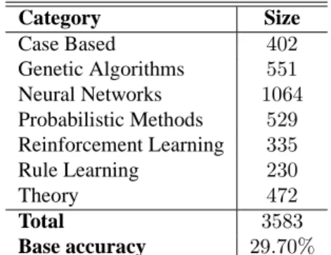
Category Size Case Based 402 Genetic Algorithms 551 Neural Networks 1064 Probabilistic Methods 529 Reinforcement Learning 335 Rule Learning 230 Theory 472 Total 3583 Base accuracy 29.70%

Table 6: Details on class distribution for the CoRA data set.

3.1.2 CORA

The CoRA data set (McCallum et al., 2000) comprises computer science research papers. It includes the full citation graph as well as labels for the topic of each paper (and potentially sub- and sub-sub-topics).12 Following a prior study (Taskar et al., 2001), we focused on papers within the machine learning topic with the classification task of predicting a paper’s sub-topic (of which there are seven). The class distribution of the data set is shown in Table 6.

Papers can be linked in one of two ways: they share a common author, or one cites the other. Following prior work (Lu and Getoor, 2003), we link two papers if one cites the other. This number ordinarily would only be zero or one unless the two papers cite each other.

3.1.3 WEBKB

The third domain we draw from is based on the WebKB Project (Craven et al., 1998).13 It consists of sets of web pages from four computer science departments, with each page manually labeled into7

categories: course, department, faculty, project, staff, student or other. As with other work (Neville et al., 2003; Lu and Getoor, 2003), we ignore pages in the “other” category except as described below.

From the WebKB data we produce eight networked data sets for within-network classification. For each of the four universities, we consider two different classification problems: the 6 class problem, and following a prior study, the binary classification task of predicting whether a page belongs to a student (Neville et al., 2003).14 The binary task results in an approximately balanced class distribution.

Following prior work on web-page classification, we link two pages by co-citations (ifxlinks tozandylinks toz, thenxandyare co-citingz) (Chakrabarti et al., 1998; Lu and Getoor, 2003). To weight the link betweenxandy, we sum the number of hyperlinks fromxtozand separately the number fromytoz, and multiply these two quantities. For example, if student xhas2edges to a group page, and a fellow studentyhas3edges to the same group page, then the weight along that path between those2students would be6. This weight represents the number of possible co-citation paths between the pages. Co-co-citation relations are not uniquely useful to domains involving documents; for example, as mentioned above, for phone-fraud detection bandits often call the same

12. These labels were assigned by a naive Bayes classifier (McCallum et al., 2000). 13. We use the WebKB-ILP-98 data.

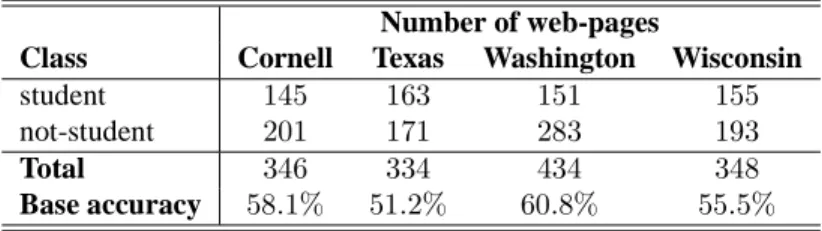
Number of web-pages

Class Cornell Texas Washington Wisconsin

student 145 163 151 155

not-student 201 171 283 193

Total 346 334 434 348

Base accuracy 58.1% 51.2% 60.8% 55.5%

Table 7: Details on class distribution for the WebKB data set using binary class labels.

Number of web-pages

Category cornell texas washington wisconsin

course 54 51 170 83 department 25 36 20 37 faculty 62 50 44 37 project 54 28 39 25 staff 6 6 10 11 student 145 163 151 155 Total 346 334 434 348 Base accuracy 41.9% 48.8% 39.2% 44.5%

Table 8: Details on class distribution for the WebKB data set using6-class labels.

numbers as previously identified bandits. We chose co-citations for this case study based on the prior observation that a student is more likely to have a hyperlink to her advisor or a group/project page rather than to one of her peers (Craven et al., 1998).15

To produce the final data sets, we extracted the pages that have at least one incoming and one outgoing link. We removed pages in the “other” category from the classification task, although they were used as “background” knowledge—allowing2pages to be linked by a path through an “other” page. For the binary tasks, the remaining pages were categorized into either student or not-student. The composition of the data sets is shown in Tables 7 and 8.

3.1.4 INDUSTRYCLASSIFICATION

The final domain we draw from involves classifying public companies by industry sector. Compa-nies are linked via cooccurrence in text documents. We create two different data sets, representing different sources and distributions of documents and different time periods (which correspond to different topic distributions).

INDUSTRYCLASSIFICATION(YH)

As part of a study of activity monitoring (Fawcett and Provost, 1999), Fawcett and Provost collected22,170business news stories from the web between 4/1/1999 and 8/4/1999. Following the study by Bernstein et al. (2003) discussed above, we identified the companies mentioned in each story and added an edge between two companies if they appeared together. The weight of an edge is the number of such cooccurrences found in the complete corpus. The resulting network comprises

15. We return to these data in Section 3.3.5, where we show and discuss how using the hyperlinks directly is not sufficient for any of the univariate methods to do well.

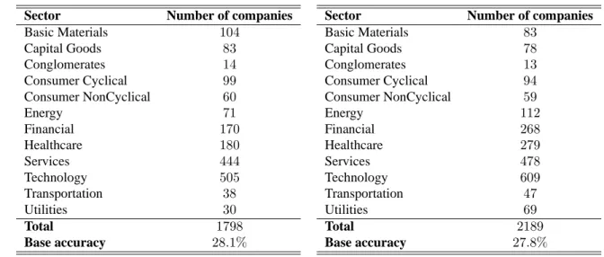
Sector Number of companies Basic Materials 104 Capital Goods 83 Conglomerates 14 Consumer Cyclical 99 Consumer NonCyclical 60 Energy 71 Financial 170 Healthcare 180 Services 444 Technology 505 Transportation 38 Utilities 30 Total 1798 Base accuracy 28.1%

Table 9: Details on class distribution for industry-yh data set.

Sector Number of companies

Basic Materials 83 Capital Goods 78 Conglomerates 13 Consumer Cyclical 94 Consumer NonCyclical 59 Energy 112 Financial 268 Healthcare 279 Services 478 Technology 609 Transportation 47 Utilities 69 Total 2189 Base accuracy 27.8%

Table 10: Details on class distribution for the industry-pr data set.

1798companies which cooccurred with at least one other company. To classify a company, we used Yahoo!’s12industry sectors. Table 9 shows the details of the class memberships.

INDUSTRYCLASSIFICATION(PR)

The second Industry Classification data set is based on35,318prnewswire press releases gath-ered from April 1, 2003 through September 30, 2003. As above, the companies mentioned in each press release were extracted and an edge was placed between two companies if they appeared to-gether in a press release. The weight of an edge is the number of such cooccurrences found in the complete corpus. The resulting network comprises2189companies which cooccurred with at least one other company. To classify a company, we use the same classification scheme from Yahoo! as before. Table 10 shows the details of the class memberships.

3.2 Experimental Methodology

NetKit allows for any combination of a local classifier (LC), a relational classifier (RC) and a collec-tive inferencing method (CI). If we consider an LC-RC-CI configuration to be a complete network-classification (NC) method, we have12to compare on each data set. Since, for this paper, the LC component is directly tied to the CI component, we henceforth consider an NC system to be an RC-CI configuration.

We first verify that the network structure alone (linkages plus known class labels) often contains a considerable amount of useful information for entity classification. To that end, we assess the classification performance of each NC as we vary from10% to 90% the percentage of nodes in the network for which class membership is known initially. Varying the amount of information initially available assesses: (1) whether the network structure enables classification; (2) how much prior information is needed in order to perform well, and (3) whether there are regular patterns of improvement with more labeled entities.

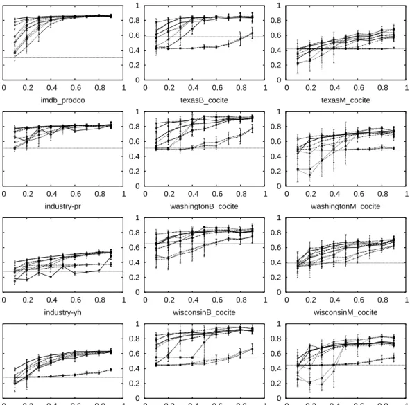
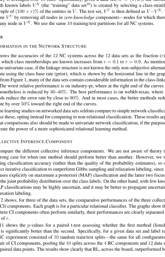
0 0.2 0.4 0.6 0.8 1 0 0.2 0.4 0.6 0.8 1 Accuracy CoRA_cite 0 0.2 0.4 0.6 0.8 1 0 0.2 0.4 0.6 0.8 1 cornellB_cocite 0 0.2 0.4 0.6 0.8 1 0 0.2 0.4 0.6 0.8 1 cornellM_cocite 0 0.2 0.4 0.6 0.8 1 0 0.2 0.4 0.6 0.8 1 Accuracy imdb_prodco 0 0.2 0.4 0.6 0.8 1 0 0.2 0.4 0.6 0.8 1 texasB_cocite 0 0.2 0.4 0.6 0.8 1 0 0.2 0.4 0.6 0.8 1 texasM_cocite 0 0.2 0.4 0.6 0.8 1 0 0.2 0.4 0.6 0.8 1 Accuracy industry-pr 0 0.2 0.4 0.6 0.8 1 0 0.2 0.4 0.6 0.8 1 washingtonB_cocite 0 0.2 0.4 0.6 0.8 1 0 0.2 0.4 0.6 0.8 1 washingtonM_cocite 0 0.2 0.4 0.6 0.8 1 0 0.2 0.4 0.6 0.8 1 Accuracy Ratio Labeled industry-yh 0 0.2 0.4 0.6 0.8 1 0 0.2 0.4 0.6 0.8 1 Ratio Labeled wisconsinB_cocite 0 0.2 0.4 0.6 0.8 1 0 0.2 0.4 0.6 0.8 1 Ratio Labeled wisconsinM_cocite

Figure 1: Overall classification accuracies on the twelve data sets. Horizontal lines represent predicting the most prevalent class. Individual methods will be clarified in subsequent figures. The horizontal axis plots the fraction (r) of a network’s nodes for which the class label is known ex ante. In each case, when many labels are known (right end) there is a set of methods that performs well. When few labels are known (left end) there is much more variation in performance. Data sets are tagged based on the edge-type used, where ‘prodco’ is short for ‘production company’, and ‘B’ and ‘M’ in the WebKB data sets represents ‘binary’ and ‘multi-class’ classifications, respectively.

Accuracy is averaged over 10 runs. Specifically, given a data set,G = (V, E), the subset of entities with known labelsVK _{(the “training” data set}16_{) is created by selecting a class-stratified}

random sample of(100×r)%of the entities inV. The test set,VU _{is then defined asV−V}K_{. We}

further pruneVU _{by removing all nodes in zero-knowledge components—nodes for which there is}

no path to any node inVK_{. We use the same10training/test partitions for all NC systems.} 3.3 Results

3.3.1 INFORMATION IN THENETWORKSTRUCTURE

Figure 1 shows the accuracies of the12 NC systems across the12data sets as the fraction (r) of entities for which class memberships are known increases fromr = 0.1tor = 0.9. As mentioned above, in the univariate case, if the linkage structure is not known the only non-subjective alternative is to estimate using the class base rate (prior), which is shown by the horizontal line in the graphs. As is clear from Figure 1, many of the data sets contain considerable information in the class-linkage structure. The worst relative performance is on industry-pr, where at the right end of the curves the error rate nonetheless is reduced by30–40%. The best performance is on webkb-texas, where the best methods reduce the error rate by close to90%. And in most cases, the better methods reduce the error rate by over50%toward the right end of the curves.

Machine learning studies on networked data sets seldom compare to simple network-classification methods like these, opting instead for comparing to non-relational classification. These results argue strongly that comparisons also should be made to univariate network classification, if the purpose is to demonstrate the power of a more sophisticated relational learning method.

3.3.2 COLLECTIVEINFERENCECOMPONENT

We now compare the different collective inference components. We are not aware of theory that makes a strong case for when one method should perform better than another. However, we will be comparing classification accuracy (rather than the quality of the probability estimates), so one might expect iterative classification to outperform Gibbs sampling and relaxation labeling, since the former focuses explicitly on maximum a posteriori (MAP) classification and the latter two focus on estimating the joint probability distribution over the class labels. On the other hand, with few known labels, MAP classifications may be highly uncertain, and it may be better to propagate uncertainty, as does relaxation labeling.

Figure 2 shows, for three of the data sets, the comparative performances of the three collective inference (CI) components. Each graph is for a particular relational classifier. The graphs show that, while the three CI components often perform similarly, their performances are clearly separated for low values ofr.

Table 11 shows the p-values for a paired t-test assessing whether the first method (listed in column 1) is significantly better than the second. Specifically, for a given data set and label ratio (r), each NC experiment consisted of10random train/test splits—the same for all configurations. For each pair of CI components, pooling the10splits across the4RC components and12data sets yields480paired data points. The results show clearly that RL, across the board, outperformed both

16. These data set will be used not only for training models, but also as existing background knowledge during classifi-cation.

0 0.2 0.4 0.6 0.8 1 0 0.2 0.4 0.6 0.8 1 Accuracy CoRA_cite - wvRN RL IC GS 0 0.2 0.4 0.6 0.8 1 0 0.2 0.4 0.6 0.8 1 imdb_prodco - wvRN RL IC GS 0 0.2 0.4 0.6 0.8 1 0 0.2 0.4 0.6 0.8 1 wisconsinB_cocite - wvRN RL IC GS 0 0.2 0.4 0.6 0.8 1 0 0.2 0.4 0.6 0.8 1 Accuracy CoRA_cite - cdRN RL IC GS 0 0.2 0.4 0.6 0.8 1 0 0.2 0.4 0.6 0.8 1 imdb_prodco - cdRN RL IC GS 0 0.2 0.4 0.6 0.8 1 0 0.2 0.4 0.6 0.8 1 wisconsinB_cocite - cdRN RL IC GS 0 0.2 0.4 0.6 0.8 1 0 0.2 0.4 0.6 0.8 1 Accuracy CoRA_cite - nBC RL IC GS 0 0.2 0.4 0.6 0.8 1 0 0.2 0.4 0.6 0.8 1 imdb_prodco - nBC RL IC GS 0 0.2 0.4 0.6 0.8 1 0 0.2 0.4 0.6 0.8 1 wisconsinB_cocite - nBC RL IC GS 0 0.2 0.4 0.6 0.8 1 0 0.2 0.4 0.6 0.8 1 Accuracy Ratio Labeled CoRA_cite - nLB RL IC GS 0 0.2 0.4 0.6 0.8 1 0 0.2 0.4 0.6 0.8 1 Ratio Labeled imdb_prodco - nLB RL IC GS 0 0.2 0.4 0.6 0.8 1 0 0.2 0.4 0.6 0.8 1 Ratio Labeled wisconsinB_cocite - nLB RL IC GS

Figure 2: Comparison of Collective Inference methods on a select few data sets, with data set and RC component listed above each graph. The horizontal line represents predicting the most prevalent class.

GS and IC, often atp≤0.001. Further, we see that IC also was often better than GS, although not always significantly.

The foregoing shows that relaxation labeling is consistently better when the results are pooled across CI pairs. Table 12 shows the magnitude of the differences. In order to be comparable across data sets with different base rates, the table shows how much of an error reduction over the base rate the first method (listed first in column 1) produces as compared to the second (listed second in column 1). As a simple example, assume the base error rate is0.4, method A yields an error rate of0.1, and method B yields an error rate of0.2. Method A reduces the error by75%. Method B reduces the error by50%. The relative error reduction of A vs. B is1.5(50%more error reduction). More precisely, for each labeling ratio r, we computed the relative error reduction ratio, ER∗_REL,

sample ratio

0.10 0.20 0.30 0.40 0.50 0.60 0.70 0.80 0.90 RL v GS 0_.001 0_.001 0_.001 0_.001 0_.001 0_.001 0_.001 0_.001 0_.001 RL v IC 0_.001 0_.001 0_.100 0_.025 0_.001 0_.001 0_.001 0_.001 0_.001 IC v GS 0.200 0_.300 0_.100 0_.050 _0.450 0_.200 0_.100 0_.005 0_.250

Table 11: p-values for the statistical significance in differences in performance between pairs of CI components across all data sets and RC methods. For each cell, bold text means that the first method was better than the second method and italics means it was worse.

sample ratio

0.10 0.20 0.30 0.40 0.50 0.60 0.70 0.80 0.90 overall RL v GS 2_.790 1_.462 1_.136 1_.124 1_.063 1_.061 1_.042 1_.035 1_.014 1_.093 RL v IC 404_.315 1_.593 1_.115 1_.078 1_.072 1_.055 1_.037 1_.018 1_.013 1_.098 IC v GS 144.937 1.090 1_.019 1_.043 1.009 1_.005 1_.005 1_.016 1_.002 1.004 Table 12: Relative error reduction (ER∗_REL) improvements for each CI component across all data sets. Each cell shows the ratio of the better method’s error reduction over the other method’s error reduction. As above, bold text means that the first method was better than the second, and italics mean it was worse. The last column, overall, is based on taking the ratio of the average error reduction for the methods across all sample ratios.

between two components, CIAand CIBas follows.

ERABS(RC,CI, D, r) = (base err(D)−err(RC-CI, D, r)) (12) ERREL(RC,CI, D, r) =

(

NA if ERABS(RC,CI, D, r)<0

ERABS(RC,CI,D,r)

base err(D) otherwise

(13) ERREL(RC,CI, r) = 1 |D_| X D∈D ERREL(RC,CI, D, r) (14) ERREL(CI, r) = 1 |RC_| X RC∈RC ERREL(RC,CI, r) (15) ER∗_REL(CIA,CIB, r) = ( ∞ if ERREL(CIB, r) =NA or0 ERREL(CIA,r) ERREL(CIB,r) otherwise (16) (17) where err(RC-CI,D, r) is the error for the configuration (RC and CI) on data setDwithr%of the graph being labelled. A ratioρ > 1means that CIAreduced the error by(100×(1−ρ))%over

that of CIB.

Table 12, following the same layout as Table 11, shows the ratios for each CI comparison. The unusually large entries occur when ERREL(CIB, r)is very close to zero. As is clear from this table,

RL outperformed IC across the board, from as low as a1.3%improvement (r = 0.90) to as high as

sample ratio

0.10 0.20 0.30 0.40 0.50 0.60 0.70 0.80 0.90 total

RL 11 11 10 7 4 5 6 4 6 64

GS 1 1 0 1 5 3 4 4 4 23

IC 0 0 2 4 3 4 2 4 2 21

Table 13: Number of times each CI method was the best across the12data sets.

RL improved performance over IC by about10%as seen in the last column in the “RL v IC” row of the table. RL’s advantage over IC improves monotonically as less is known in the network. Similar numbers and a similar pattern are seen for RL versus GS. IC and GS are comparable.17

The results so far have compared the CI methods disregarding the RC component. Table 13 shows, for each ratio as well as a total across all ratios, the number of times each CI implementation took part in the best-performing NC combination for each of the twelve data sets. Specifically, for each sampling ratio, each win for an RC-CI configuration counted as a win for the CI module of the pair (as well as a win for the RC module in the next section). For example, in Figure 2, the first column of four graphs shows the performances of the 12 NC combinations on the CoRA data; at the left end of the curves, wvRN-RL is the best performing combination. Table 13 adds further support to the conclusion that relaxation labeling (RL) was the overall best component, primarily due to its advantage at low values ofr. We also see again that Gibbs Sampling (GS) and Iterative Classification (IC) were comparable.

3.3.3 RELATIONALMODELCOMPONENT

Comparing relational models, we would expect to see a certain pattern: if even moderate homophily is present in the data, we would expect wvRN to perform well. Its nonexistent training variance18 should allow it to perform relatively well, even with small numbers of known labels in the network. The higher-variance nLB may perform relatively poorly with small numbers of known labels (pri-marily because of the lack of training data, rather than problems with collective inference). On the other hand, wvRN is potentially a very-high-bias classifier (it does not learn at all). The learning-based classifiers may well perform better with large numbers of known labels if there are patterns beyond homophily to be learned. As a worst case for wvRN, consider a bipartite graph between two classes. In a leave-one-out cross-validation, wvRN would be wrong on every prediction. The relational learners should notice the true pattern immediately.

Figure 3 shows for four of the data sets the performances of the four RC implementations. The rows of graphs correspond to data sets and the columns to the three different collective inference methods. The graphs show several things, which will be clarified next. As would be expected, accuracy improves as more of the network is labeled, although in certain cases classification is remarkably accurate with very few known labels (e.g., see CoRA). One method is substantially worse than the others. Among the remaining methods, performance often differs greatly with few known labels, and tends to converge with many known labels. More subtly, there often is a crossing of curves when about half the nodes are labeled (e.g., see Washington).

17. NB: it is possible for the winner in Table 11 and the winner in Table 12 to disagree (as seen for the IC and GS comparisons atr _{= 0}._{20), because the relative error reduction depends on the base error whereas the statistical test} is based on the absolute values.

sample ratio 0.10 0.20 0.30 0.40 0.50 0.60 0.70 0.80 0.90 wvRN v cdRN 0_.001 0_.001 0_.001 0_.001 0_.001 0_.001 0_.001 0_.001 0_.001 wvRN v nBC 0_.001 0_.001 0_.001 0_.001 0_.001 0_.001 0_.001 0_.001 0_.001 wvRN v nLB 0_.001 0_.001 0_.001 0_.001 _{0.300 0.001 0.001 0.001 0.001} cdRN v nBC 0_.001 0_.001 0_.001 0_.001 0_.001 0_.001 0_.001 0_.001 0_.001 cdRN v nLB 0_.001 0_.001 0_.001 0_.001 0.002 0.001 0.001 0.001 0.001 nLB v nBC 0.250 0_.010 0_.001 0_.001 0_.001 0_.001 0_.001 0_.001 0_.001

Table 14: p-values for the statistical significance of differences in performance among the RC com-ponents across all data sets. For each cell, bold text means that the first method was better than the second method and italic text means it was worse.

sample ratio

0.10 0.20 0.30 0.40 0.50 0.60 0.70 0.80 0.90 overall wvRN v cdRN 1_.483 1_.092 1_.059 1_.070 1_.042 1_.058 1_.047 1_.057 1_.040 1_.068 wvRN v nLB ∞ 7_.741 1_.901 1_.279 _{1.027 1.091 1.081 1.082 1.067} 1_.163 cdRN v nLB ∞ 7_.086 1_.794 1_.195 _{1.071 1.154 1.132 1.144 1.110} 1_.089

Table 15: Relative error reduction (ER∗_REL) improvements for each RC component across all data sets. Each cell shows the ratio of the better method’s error reduction over the other method’s error reduction. The last column, overall, is based on taking the ratio of the average error reduction for the methods across all sample ratios. Bold text means the first method is better and italics means the second method is better.∞means that the second method performed worse than the base error.

sample ratio

0.10 0.20 0.30 0.40 0.50 0.60 0.70 0.80 0.90 total

wvRN 7 4 4 6 4 4 2 1 2 34

cdRN 5 8 6 2 1 0 0 1 1 24

nLB 0 0 2 4 7 8 10 10 9 50

0 0.2 0.4 0.6 0.8 1 0 0.2 0.4 0.6 0.8 1 Accuracy CoRA_cite - RL wvRN cdRN nBC nLB 0 0.2 0.4 0.6 0.8 1 0 0.2 0.4 0.6 0.8 1 CoRA_cite - GS wvRN cdRN nBC nLB 0 0.2 0.4 0.6 0.8 1 0 0.2 0.4 0.6 0.8 1 CoRA_cite - IC wvRN cdRN nBC nLB 0 0.2 0.4 0.6 0.8 1 0 0.2 0.4 0.6 0.8 1 Accuracy industry-yh - RL wvRN cdRN nBC nLB 0 0.2 0.4 0.6 0.8 1 0 0.2 0.4 0.6 0.8 1 industry-yh - GS wvRN cdRN nBC nLB 0 0.2 0.4 0.6 0.8 1 0 0.2 0.4 0.6 0.8 1 industry-yh - IC wvRN cdRN nBC nLB 0 0.2 0.4 0.6 0.8 1 0 0.2 0.4 0.6 0.8 1 Accuracy cornellM_cocite - RL wvRN cdRN nBC nLB 0 0.2 0.4 0.6 0.8 1 0 0.2 0.4 0.6 0.8 1 cornellM_cocite - GS wvRN cdRN nBC nLB 0 0.2 0.4 0.6 0.8 1 0 0.2 0.4 0.6 0.8 1 cornellM_cocite - IC wvRN cdRN nBC nLB 0 0.2 0.4 0.6 0.8 1 0 0.2 0.4 0.6 0.8 1 Accuracy Ratio Labeled washingtonB_cocite - RL wvRN cdRN nBC nLB 0 0.2 0.4 0.6 0.8 1 0 0.2 0.4 0.6 0.8 1 Ratio Labeled washingtonB_cocite - GS wvRN cdRN nBC nLB 0 0.2 0.4 0.6 0.8 1 0 0.2 0.4 0.6 0.8 1 Ratio Labeled washingtonB_cocite - IC wvRN cdRN nBC nLB

Figure 3: Comparison of Relational Classifiers on a select few data sets. The data set (and link-type) and the paired collective inference component is listed above each graph. The horizontal line represents predicting the most prevalent class.

Table 14 shows statistical significance results, computed as described in the previous section (except here varying the RC component). Clearly, nBC was always significantly worse than the other three RCs and is therefore eliminated from the remainder of this analysis. wvRN was always significantly better than cdRN. Examining the two RN methods versus nLB we see the same pattern: atr= 0.5, the advantage shifts from the RN methods to nLB.

Table 15 shows the error reduction ratios for each RC comparison, computed as in the previous section with the obvious changes between RC and CI. The same patterns are evident as observed from Table 14. Further, we see that the differences can be large: when the RN methods are better, they often are much better. The link-based classifier also can be considerably better than wvRN— however, we should keep in mind that wvRN does not learn!