HIGH DENSITY RATIO MULTI-COMPONENT LATTICE BOLTZMANN FLOW MODEL FOR FLUID DYNAMICS AND CUDA PARALLEL COMPUTATION
by Jie Bao
BS, Beijing University of Aeronautics and Astronautics, China, 2004
Submitted to the Graduate Faculty of
Swanson School of Engineering in partial fulfillment of the requirements for the degree of
Doctor of Philosophy
University of Pittsburgh 2010
UNIVERSITY OF PITTSBURGH SWANSON SCHOOL OF ENGINEERING
This dissertation was presented by
Jie Bao
It was defended on Feburary 26th, 2010
and approved by
Dr. Anne M. Robertson, Associate Professor, Department of Mechanical Engineering & Materials Science Dr. Sung K. Cho, Associate Professor, Department of Mechanical Engineering & Materials Science
Dr. Joseph J. McCarthy, Associate Professor, Department of Chemical & Petroleum Engineering Dissertation Director: Dr. Laura Schaefer, Associate Professor,
Copyright © by Jie Bao 2010
HIGH DENSITY RATIO MULTI-COMPONENT LATTICE BOLTZMANN FLOW MODEL FOR FLUID DYNAMICS AND CUDA PARALLEL COMPUTATION
Jie Bao, PhD
University of Pittsburgh, 2010
The lattice Boltzmann equation (LBE) method is a promising technique for simulating fluid flows and modeling complex physics in fluids, and can be modified for solving general nonlinear partial differential equations (NPDEs). The LBE method has recently attracted more and more attention since it may help us to better understand the mechanisms of the complicated physical phenomena and dynamic processes modeled by NPDEs.
In this dissertation, firstly, we developed a second-order accurate mass conserving boundary condition (BC) for the LBE method. Through several cases, the results show that our mass conserving BC will not result in the constant mass leakage that occurs for the other BCs in some cases. Additionally, it increases the efficiency and stability of the method for cases that involve relatively large magnitudes of body force.
Secondly, we developed a multi-component and multi-phase LBE method for high density ratios. Multi-component multi-phase (MCMP) flow is very common in engineering or industrial problems and in nature. Because the lattice Boltzmann equation (LBE) model is based on microscopic models and mesoscopic kinetic equations, it offers many advantages for the study of multi-component or multi-phase flow problems. While the original formulation of Shan and Chen’s (SC) model can incorporate some multiple phase and component scenarios, the density ratio of the different components is greatly restricted (less than approximately 2.0). This obviously limits the applications of this MCMP LBE model. Hence, based on the original SC
MCMP model and the improvements in the single-component multi-phase (SCMP) flow model reported by Yuan and Schaefer, we have developed a new model that can simulate a MCMP system with a high density ratio.
Finally, we developed a parallel computation LBE method based on Compute Unified Device Architecture (CUDA). CUDA offers a great economic alternative way to increase the calculation speed of LBE method instead of using a supercomputer. We present how to apply CUDA to the LBE method, including boundary condition treatments, single phase flow, thermal problems, and multi-phase cases. Through the results of several numerical experiments, our model with the help of CUDA can offer an improvement of a 10-30 times faster speed than that of a traditional single thread CPU code.
TABLE OF CONTENTS
1.0 INTRODUCTION... 1
1.1 INTRODUCTION TO THE LATTICE BOLTZMANN EQUATION METHOD 2 1.2 INTRODUCTION TO THE MULTI-PHASE LBE METHOD ... 6
1.3 INTRODUCTION TO THE THERMAL LBE METHOD... 9
2.0 INTRODUCTION TO BOUNDARY CONDITIONS FOR THE LBE METHOD... 11
2.1 BOUNCE BACK SOLID WALL BOUNDARY CONDITIONS... 11
2.2 CURVED SOLID WALL BOUNDARY CONDITIONS ... 14
2.3 THE OPEN BOUNDARY CONDITION... 17
2.3.1 Periodical Boundary Condition ... 17
2.3.2 Extrapolation Boundary Condition ... 18
2.3.3 Inlet Boundary Condition... 19
2.3.4 Thermal Boundary Condition... 21
3.0 A MASS CONSERVING BOUNDARY CONDITION FOR THE LBE METHOD... 24
3.1 FULLY DEVELOPED FLOW IN A 2-D CURVED PIPE ... 24
3.2 STEADY AND UNSTEADY FLOW OVER A CIRCULAR CYLINDER ... 27
3.3 CONCLUSION AND DISCUSSION... 32
4.0 THE LBE METHOD FOR MULTI-COMPONENT MULTI-PHASE FLOW WITH HIGH DENSITY RATIOS ... 35
4.2 SIMULATION OF AN EQUILIBRIUM DROPLET WITHOUT A BODY
FORCE AND EXTERNAL FORCES ... 37
4.2.1 Maximum Force Ratio ... 39
4.2.2 Spurious Current... 44
4.2.3 Convergence Speed... 47
4.3 SIMULATION OF AN EQUILIBRIUM DROPLET AFFECTED BY A BODY FORCE AND EXTERNAL FORCES ... 48
4.4 SIMULATION OF A DROPLET IN A FLOW ... 50
4.5 CONCLUSIONS AND DISCUSSION ... 51
5.0 APPLICATION OF THE COMPUTE UNIFIED DEVICE ARCHITECTURE (CUDA) TO THE LATTICE BOLTZMANN EQUATION METHOD ... 53
5.1 BRIEF INTRODUCTION TO PARALLEL COMPUTATION FOR THE LBE METHOD ... 53
5.2 INTRODUCTION TO THE CUDA LBE METHOD... 56
5.3 INTRODUCTION TO THE CUDA PROGRAMMING STRATEGY FOR THE LBE METHOD ... 61
5.4 EXPERIMENTAL METHODOLOGY AND RESULTS ... 70
5.4.1 Methodology... 70
5.4.2 Single Component Single Phase Flow... 71
5.4.3 Thermal Single Component Single Phase Flow... 78
5.4.4 Multi-Phase Flow... 82
5.5 CONCLUSIONS AND DISCUSSION ... 92
6.0 CONCLUSIONS AND FUTURE WORK ... 94
6.1 MAJOR ACCOMPLISHMENTS ... 94
6.2 FUTURE WORK ... 96
APPENDIX A. EXAMPLE OF CUDA CODES ... 98
APPENDIX C. FROM THE CONTINUUM BOLTZMANN EQUATION TO THE LBE MODEL ... 108 BIBLIOGRAPHY ... 112
LIST OF TABLES
1 NVIDIA Geforce graphic cards ... 59 2 GPU Specifications... 71 3 Calculation time comparison between isothermal and thermal LBE models... 80
LIST OF FIGURES
1.1 The 2D grids for LBM ... 3
1.2 2D square lattice and 3D cubic lattice for LBM ... 5
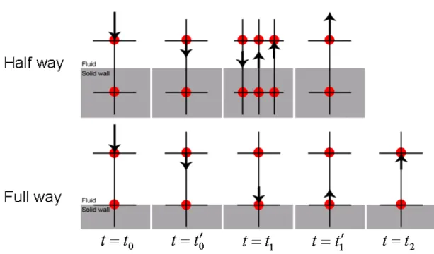
2.1 Demonstration of half way and full way bounce back boundary condition ... 12
2.2 Demonstration of 2-D LBE grids, (a) low resolution, (b) high resolution ... 14
2.3 Layout of the lattice and curved wall boundary... 15
2.4 PDFs of a flat boundary site at the lower wall boundary after the streaming step ... 17
2.5 Layout of the inlet boundary... 19
2.6 Configuration of PDFs used to construct the inlet boundary condition... 20
2.7 Sketch of thermal boundary condition for D2Q9 ... 22
3.1 Schematic computational area for flow in a curved pipe... 25
3.2 Flow in a curved pipe... 26
3.3 System mass change with time using the mass conserving BC and MLS BC ... 27
3.4 Schematic of the computational area for steady flow over a circular cylinder... 28
3.5 Steady flow around a cylinder at Re=10, with streamlines and pressure contours... 29
3.6 Comparison of the velocity profiles at x=0... 30
3.7 Comparison of the velocity variation at the centerline (y=0) for the MLS BC, mass conserving BC and finite difference result for Re=10... 31
3.8 Unsteady flow around a cylinder at Re=100... 32
4.1 (a) Density contour for a circular droplet, (b) Comparison of the densities of the two components along the center line (y50, 0x100)... 39
4.2 Distribution of the ratio of F1,1x and F1,1,max... 40
4.3 Comparison of the density of the two components along the center ... 42
4.4 Density ratio 2 1 Component Component variation with the ratio of the maximum force max 2 , 1 max 1 , 1 F F ... 44
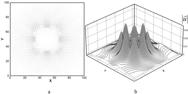
4.5 (a) Vector of spurious current around the droplet, (b) magnitude of the spurious current .... 45
4.6 The maximum magnitude of the spurious currents varying with the density ratio ... 46
4.7 The residual changes with time steps... 48
4.8 Position of the interface of the two components on a hydrophilic and hydrophobic surface, and comparison of the density of the two components along the center line (x50, ) ... 50
100 0y 4.9 Position of interface of the two components and velocity vector,... 51
5.1 Comparison of runtime performance for a different number of cores on a 64X64X64 LBE problem for the (a) Intel Core 2 and (b) AMD OpternX2 ... 55
5.2 Price comparison for multi-core computer systems... 55
5.3 Modern supercomputer architecture ... 56
5.4 Comparison of floating-point operation capacity between GPUs and CPUs ... 57
5.5 Structural organization of a CPU and a GPU, (a) CPU, (b) GPU ... 58
5.6 (a) NVIDIA SLI system; (b) NVIDIA Tesla Computing System ... 59
5.7 Comparison of memory bandwidth for different system... 61
5.8 General programming strategy for numerical simulation based on CUDA ... 63
5.9 Division of blocks: a, 4 blocks; b, 8 blocks ... 65
5.10 Demonstration of block division for CUDA... 65
5.11 Streaming step: (a) time step 0; (b) time step 1 ... 67
5.12 Demonstration of the streaming step and collision step based on the CUDA LBE model . 67 5.13 Grids for calculating the gradient term of effective mass... 69
5.15 Demonstration of the Thermal LBE model based on CUDA programming ... 70
5.16 Comparison of velocity profile from CUDA LBE model (red vectors) and analytical solution (blue line) ... 72
5.17 Calculation time comparison between GPUs and CPUs ... 73
5.18 Calculation time (in ms) for different size of block... 74
5.19 (a) Demonstration of simulation domain, (b) Velocity profile on a slice at y=25... 75
5.20 Calculation time comparison for 3-D porous media flow ... 75
5.21 (a) Simulation domain for flow in vessel networks, (b) streamline in blood vessel from the LBE model, (c) streamline in blood vessel from a finite element analysis method ... 77
5.22 (a) Demonstration of simulation domain, (b) Temperature contour on a slice at y=25... 81
5.23 Temperature contour at the slice of y=20 for time steps 200, 400, 800 and 1200... 81
5.24 Calculation time comparison for 3-D thermal porous media flow ... 82
5.25 A droplet on a micro-structured solid surface... 83
5.26 (a) liquid droplet on hydrophobic surface, (b) a cross section of droplet ... 84
5.27 Computer graphic of a lotus leaf surface ... 85
5.28 Droplet on hydrophilic surface ... 86
5.29 A cross section of droplet on hydrophilic surface ... 86
5.30 Calculation time comparison for 3-D multi-phase flow ... 87
5.31 (a) SEM image of nanowire array, (b) schematic diagram of ideal ZnO nanocomposite, (c)(d) SEM image of ZnO nanocomposites... 88
5.32 Sketch of the simulation domain... 89
5.33 (a) Cross section and liquid interface of droplet for repulsive interaction, (b) cross section and liquid interface of droplet for attractive interaction ... 90
NOMENCLATURE Roman Letters
a, Acceleration; attraction parameter in equation of state a b Repulsion parameter in equation of state
c Lattice speed; lattice spacing
0
c Constant in equation of state
s
c Lattice sound speed D Dimension of space
e Lattice velocity vector
f Particle distribution function
eq
f Equilibrium particle distribution function F Force per unit mass
g Gravitational constant; fluid-fluid interaction strength
f
g Intensity of fluid-fluid interaction
w
g Intensity of fluid-solid interaction H Height of the domain
L Length of the domain
nx,ny, nz Lattice size in the x, y and z directions p Pressure
Re Reynolds number t Time T Temperature u, Fluid velocity u eq u Equilibrium velocity x Position Greek Letters t Time step x, y Lattice constant Relaxation time Dynamic viscosity Kinematic viscosity Discrete velocity set Density w Wall density Relaxation time Effective mass Abbreviations BC Boundary condition BGK Bhatnagar-Gross-Krook CFD Computational fluid dynamics
CUDA Compute unified device architecture EOS Equation of state
FH Filippova and Hänel LB Lattice Boltzmann
LBE Lattice Boltzmann equation LBGK Lattice BGK
MLS Mei, Luo, and Shyy N-S Navier-Stokes
NPDE nonlinear partial differential equation PDE Partial differential equation
PDF Particle distribution function SC Shan & Chen
ACKNOWLEDGEMENTS
During my Ph.D. study work, many people helped me in numerous ways. Let me try to thank them without, I hope, forgetting anyone.
First and foremost, I with to acknowledge my advisor, Dr. Laura Schaefer, for supporting me, encouraging me and guiding me throughout my whole Ph. D. study and research work with her brilliant advice, patience and kindness. Thank you.
My thanks are extended to the members of my thesis committee, Drs. Anne M. Robertson, Joseph J. McCarthy and Sung K. Cho. Thank you for your time and valuable advice. I am very thankful to the faculty and staff members in the Department of Mechanical Engineering, who have made my studies here valuable and enjoyable.
Special thanks go to Dr. Peng Yuan for the cooperation and helpful suggestions and discussions.
Thanks also go to Zijing Zeng for the useful suggestions and discussions.
I feel lucky to have made a lot of new friends here. My life becomes happy in Pitt due to the following people: Lifeng Qin, Di Xu, Yunjun Zhao, Chunhua Fu, Dr. Hongbin Cheng, Dr. Qingming Chen, Tony Kerzmann, Veronica Miller, Michael Ikeda, Dr. Florian Zink.
I reserve my sincere thanks for my family members. I am deeply indebted to my father: Qixiong Bao, and my mother Yufang Ding for their support and endless love through my whole life and the long journey of study. Words cannot express the gratitude I have to what they have
done for me in the past. I am also thankful for the love and encouragements provided by my wife’s parents.
Finally, I would like to thank my wife Kun Li for support and faith in me. Thank you for sharing with me all the exciting and difficult times of living and studying in a foreign country.
1.0 INTRODUCTION
The lattice Boltzmann equation (LBE) method is a promising technique for simulating fluid flows and modeling complex physics in fluids. Unlike conventional computational fluid dynamics (CFD) methods, the LBE model is based on microscopic models and mesoscopic kinetic equations in which the collective behavior of the particles in a system is used to simulate the continuum mechanics of the system. Due to this kinetic nature, the LBE method has been found to be particularly useful in applications involving interfacial dynamics and complex boundaries, such as multi-phase or multi-component flows [1]. Besides that, the LBE model is straightforward to program and intrinsically parallel [2, 3, 4].
Additionally, although the LBE method can be considered to be a simplified fictitious molecular dynamics model designed for solving fluid problems, it also demonstrates the potential to simulate a nonlinear system in other areas. Some early work shows that the LBE method has been extended successfully to simulate some evolution equations [5, 6, 7, 8, 9, 10], and recent research shows that the LBE method can be used to solve more generalized nonlinear partial differential equations (NPDEs). Chai, Shi and Zheng’s work proves that the LBE model can recover 6th-order NPDEs [11]. NPDEs play an important role in different fields of physics and mathematics [12, 13], and the LBE method has therefore attracted more and more attention since it may help us to better understand the mechanisms of the complicated physical phenomena and dynamic processes modeled by NPDEs.
1.1 INTRODUCTION TO THE LATTICE BOLTZMANN EQUATION METHOD
The LBE model is derived from the continuum Boltzmann equation, which is an integro-differential equation, and describes the evolution of a single-particle distribution function
x t
f ,, in the physical-momentum space. Because of the high dimensions of the distribution and the complexity in the collision integral, direct solution of the full Boltzmann equation is a formidable task for both analytical and numerical techniques [14]. In 1954, Bhatnagar, Gross and Krook developed the Boltzmann-BGK equation which is an important simplification of the original Boltzmann equation [15]. The Boltzmann-BGK equation takes the form:
0 1 f f f t f
(1.1) For solving numerically, the Boltzmann-BGK equation is first discretized in the momentum space using a finite set of velocitiesf :
( ) 1 f f eq f t f
(1.2) where f
x,t f
x,,t and f(eq)
x,t f(0)
x, ,t
are the distribution function and the equilibrium distribution function of the th discrete velocity , respectively. The equilibrium distribution function can be expressed in the form:
u u c u e c u e c w feq 2 2 4 2 2 3 2 9 3 1 (1.3) where w is the weighting factor [16],t x c
is the lattice speed, e is the discrete velocity set, and u and are the macroscopic velocity and density.
. 8 , 7 , 6 , 5 , 1 , 1 ; 4 , 3 , 2 , 1 , 1 , 0 , 0 , 1 ; 0 , 0 , 0 c c c e (1.4) . 8 , 7 , 6 , 5 , 36 / 1 ; 4 , 3 , 2 , 1 , 9 / 1 ; 0 , 9 / 4 w (1.5)For a 3-D LBE model, the weighting factors and discrete velocities for D3Q19 (a widely used state space) are:
. 18 ,..., 8 , 7 , 1 , 1 , 0 , 1 0 , 1 , 0 , 1 , 1 ; 6 ,..., 2 , 1 1 , 0 , 0 , 0 , 1 , 0 , 0 , 0 , 1 ; 0 , 0 , 0 , 0 c c c c c c e (1.6) . 18 ,..., 8 , 7 , 36 / 1 ; 6 ,..., 2 , 1 , 18 / 1 ; 0 , 3 / 1 w (1.7)After discretizing the PDF in momentum space, the number of possible particle spatial positions and microscopic momenta are reduced to 9 for the 2-D problem, as shown in Figure 1.1. For 3-D flow, there are several cubic lattice models, such as the D3Q15, D3Q19 and D3Q27 model, as shown in Figure 1.2.
Based on the D2Q9, D3Q15, D3Q19 and D3Q27 frame definition, the density and the velocity can be defined as:
b f 0 (1.8)
b f e u 0 1 (1.9)where represents the total number of possible particle spatial positions. To solveb f
x,t , equation (1.2) needs to be further discretized in physical space x and time t, so the completely discretized form of Boltzmann-BGK equation is:
x e t t t
f
x t
f
x t f
x t
f , , 1 , eq , (1.10) where is the non-dimensional relaxation time. Appendix C shows the steps from continuum Boltzmann equation to LBE model in detail. This equation often can be solved using the following two steps [17]:Collision: ~f
x,t f
x,t 1
f
x,t feq
x,t
(1.11) Streaming: f
xet,tt
~f
x,t (1.12) After the streaming step (equation (1.12)), we can substitute the newly calculated PDF
x e t t tf ,
into equation (1.11) by replacing the old f
x,t . Every loop is a time step, and after many time steps, which may be over 10,000 for some particularly complicated phenomena, the program will converge.1.2 INTRODUCTION TO THE MULTI-PHASE LBE METHOD
It is commonly accepted that the separation of different phases or components is microscopically due to the long-range interaction between the molecules of a fluid [18]. This interaction can be expressed as:
x g
x cx
F () 0 (1.13) where is a constant depending on the lattice structure. For the D2Q9 and D3Q19 lattices,
, and for the D3Q15 lattice,
0 c 0 . 6 0
c c0 10.0 . The coefficient for the strength of the
interparticle force is g, with representing an attractive force between particles and a repulsive force.
0
g g 0
x
is the effective mass, which is a function of local density and can be varied to reflect different fluid and fluid mixture behaviors, as represented by various equations of state (EOS). This equation is derived from the original Shan and Chen (SC) model. Although that work only used the interparticle forces of nearest neighbor sites, it can be extended to include other neighboring sites as long as the gradient term is properly specified. We use both the nearest and next-nearest sites to evaluate this gradient term, which gives a six-point scheme for two dimensions:
,
1,
1,
1, 1
1, 1
1, 1
1, 1
2 1 j i j i j i j i c j i j i c
x j i (1.14a)
,
, 1
, 1
1, 1
1, 1
1, 1
1, 1
2 1 c i j i j c i j i j i j i j y j i
(1.14b) where c1 and c2 are the weighting coefficients for the nearest and next nearest sites,In addition to the interparticle forces, if the problem includes a solid wall boundary, the interaction between the fluid and solid interface needs to be considered, so the forces applied on a particle that contacts the solid wall are:
x
x G
x x
x x x
F w x w w
, (1.15)where Gw
x,x
reflects the intensity of the fluid-solid interaction, andw
x is the wall density, which equals one at the wall and zero in the fluid. Furthermore, in addition to interparticle and wall forces, the body force can be defined as:
x
x aFb (1.16) The viscosity and the surface tension are two additional important factors for specifying fluid characteristics. The viscosity is defined in the LBE model as:
t cs 2 2 1 (1.17) where is the speed of sound in the LBE model. Hence, the viscosity can be changed by choosing a different relaxation time
s
c
. In order to adjust the surface tension, an additional force term should be introduced into the fluid-fluid interaction, and is defined as:
2
s
F (1.18) where determines the strength of the surface tension [2].
Hence, the total force on each particle can be expressed as: i w b s total F F F F F (1.19) All of these forces can be incorporated into the model by shifting the velocity in the equilibrium distribution. This means that the velocity u in equation (1.3) is replaced by
x F u u i i total i i eq , (1.20) The effective mass , which was mentioned in the introduction to calculating interparticle forces and surface tension, is the mechanism for incorporating a more sophisticated EOS. As stated previously, the effective mass (x)((x)) is a function of the local density, and can be defined as:
g c c p s 0 2 2 ) ( (1.21)where p is the pressure. The choice of EOS can reflect the relationship between the pressure, temperature and density. In Yuan and Schaefer’s work [19], five different EOS were tested in this model, and it was found that that Peng-Robinson (P-R) EOS provided the maximum increase in the density ratio of SCMP flows while maintaining small spurious currents around the interface. Hence, we used the P-R EOS in our following multi-phase flow research, where the P-R EOS is expressed as:
2 2 2 2 1 ) ( 1 b b T a b RT P (1.22)
2
2 / 1 26992 . 0 5422 . 1 37464 . 0 1 ) (T T Tc (1.23) with c c P T R a 2 2 45724 . 0 and c c P RTb 0.0778 , where a is the attraction parameter, b is the volumetric or repulsion parameter, and is the acentric factor. and are the critical temperature and critical pressure, respectively.
c
1.3 INTRODUCTION TO THE THERMAL LBE METHOD
As stated previously, the LBE method can be used to solve generalized NPDEs. Hence, the LBE model can also be applied to solving thermal problems. In a single-phase thermal fluid system, if the viscous and compressive heating effects are negligible, the temperature field satisfies a much simplified passive-scalar equation:
T T u t T (1.24) where u is the macroscale velocity, is the thermal diffusivity, and is the source term. To solve equation (1.24) using the LBE method, we firstly define a particle distribution function (PDF) fT
x,t
for temperature, which is the same as the dynamic PDF. The temperature then can be found using the following relationship:
b fT T 0 (1.25) Through equations (1.26) and (1.27) below, we can solve the temperature PDF fT
x,t numerically:
x e t t t
f
x t
f
x t f
x t
f T T eq T T T , , 1 , , (1.26)
u u c u e c u e c Tw fTeq 2 2 4 2 2 3 2 9 3 1 (1.27) where T is the dimensionless single relaxation time for temperature. The temperature variance results in a buoyancy force, which is expressed as:
T T j gG 0
(1.28) To incorporate the buoyancy force, we substitute equation (1.28) into equation (1.19) (Ftotal Fi Fw Fb Fs ), calculate the total force that is applied on the particles, and thencalculate the shifted velocity by equation (1.20) (
x F u u i i total i i eq , in equation (1.27) is replaced by this shifted velocity. Through including the buoyancy force, the LBE method can be used for a number of systems with thermal effects, such as natural convection problems.
2.0 INTRODUCTION TO BOUNDARY CONDITIONS FOR THE LBE METHOD
Boundary conditions (BCs) play a very important role in numerical simulation. A BC not only affects the accuracy and stability of a computational method, but it is also one of the characteristics that determine the adaptability of a CFD method. In this section, several BCs are discussed that include most of the necessary treatments for dealing with popular practical situations, such as the solid wall BC and the open BC.
2.1 BOUNCE BACK SOLID WALL BOUNDARY CONDITIONS
In LBE simulations, to some extent, developing accurate and efficient BCs is as important as developing an accurate computation scheme itself, since they will influence the stability of the computation. The most common and simplest solid wall BC is the bounce-back boundary condition. In this BC, when a particle distribution streams to a wall node, it scatters back to the fluid node along its incoming link. However, the bounce-back BC only gives first order numerical accuracy. To improve it, many BCs have been proposed in the past [20, 21, 22, 23], such as the halfway bounce-back scheme [24, 25], which is easy to implement and gives second-order accuracy for a straight wall. In this scheme, the wall is placed halfway between a fluid node and a bounce-back node. The order of accuracy for a boundary condition in the LBE model can be tested by calculating the slope of the L2-norm error, which is defined as:
1/2 0 2 2 / 1 0 2 2
dy y u dy y u y u E H exact H exact LBE (2.1)where uLBE is the LBE solution of the velocity.
Compared with other second order boundary treatments, the halfway bounce-back does not require any extrapolation, and is therefore easy to implement. Figure 2.1 shows the application procedure of both the fullway and halfway back BC. For the halfway bounce-back BC, in only one time step, a fluid particle goes to the boundary site, reverses its velocity and comes back, while the fullway bounce-back condition needs two time steps to go forth and back. From the foundation of these simple BCs treatments, the LBE method can be used to address many complicated geometries, which is one of the strengths of the LBE model compared to traditional simulation methods.
Figure 2.2a shows an example of LBE grids for an object with a complicated geometry. From the enlargement, we can see that LBE meshes use squares to match the curved boundary. Hence, the higher the resolution (which means more grids), the better the matching between the simulation model and the real object that we are studying (such as in Figure 2.2b). This is similar to a bitmap or pixmap in computer graphics, which is a type of memory organization for an image file format that used to store digital images. Hence, for a 2D problem, for generating the grids for LBE simulation, we can firstly generate a black and white bitmap file (BMP) to describe the whole simulation domain, where a black pixel represents a solid object point and a white one a fluid space (or vice versa). Next, this image file is converted to a 2D matrix that only includes the digits 1 and 0, where 1 is black and 0 is white. The command “imread('C:\ image.bmp')” in MATLAB can easily deal with this conversion. Finally, this matrix file is defined as a solid boundary wall file in the LBE model program. By following this method, most 2D complicated geometries can be imported into the LBE simulation program.
For a 3D problem, the 3D object can be modeled in any CAD software, and then exported into an Initial Graphics Exchange Specification (IGES) file, which records the coordinates of solid object points in a 3D space. Each solid object point’s coordinate is read and recorded as 1, which is then put it in to the corresponding position in a 3D matrix. Finally, as in the 2D problem, this matrix file is defined as a solid boundary wall file in the LBE model program.
a b
Figure 2.2: Demonstration of 2-D LBE grids, (a) low resolution, (b) high resolution
2.2 CURVED SOLID WALL BOUNDARY CONDITIONS
For a curved wall, the bounce back boundary condition may result in obvious jagged boundaries when the grid’s resolution is not high enough, and therefore additional errors will be introduced. Hence, for dealing with a curved solid wall without requiring high mesh resolution, Filipova and Hänel (FH) proposed a curved wall BC [26], which later was improved by Mei, Luo and Shyy (MLS) [27, 28]. Bao, Yuan and Schaefer further refined this technique to create a mass conserving boundary condition [29] which solves the mass leakage problem of the original BC when a strong body force is present in a system.
As shown in Figure 2.3, eand e denote directions opposite to each other, xb is a boundary node, and xf is a fluid node. The curved wall is located between a boundary node and
fluid node, with
b f w f x x x x
denoting the fraction of an intersected link in the fluid region.
boundary node xb, where f~ denotes the post-collision state of the distribution function. FH proposed the following treatment for ~f(xb,t) on curved boundaries:
w b f b e u c w t x f t x f t x f )( ) ,t w 2 ) ( ( , ) 2 3 ) , ( ~ ) 1 , ( ~ 2.2) ( where uw u(x is the velocity at the wall, is the weighting factor that controls the linear interpolation between ~f(xf,t) and f( )(x ,t)
b
, and f()(xb,t) is given by a fictitious
equilibrium distribution: x t w f( )( , ) ( f f f bf w b u u c u e c u e c t x 2 2 4 2 2 3 ) ( 2 9 3 1 ) , (2.3)
where )(xw,t is called the wall density. In equation (2.3), )uf u(xf,t is the fluid velocity near the wall, ubf is to be chosen, and the weighting factor depends on ubf.
w f bf u u u [13/(2)] 3/(2) and (21)/( 1/2) for 1/2 (2.4) ) , (x e δt t u u ubf ff f f and (21)/( 2) for 1/2 (2.5)
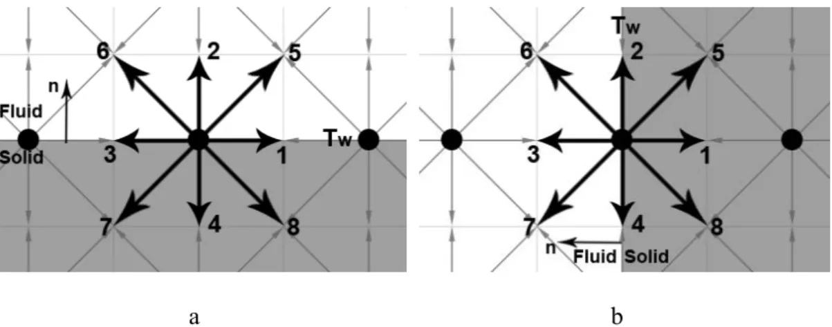
It must be determined what (xw,t) odel. Shown in
6
5 f
f
term guarantees mass conservation. We discuss this in the context of the D2Q9 m Figure 2.4 are the known and unknown PDFs of a flat boundary site at the lower wall boundary after the streaming step. The outgoing PDFs are , which are known, and the incoming PDFs are , which are unknown. Mass conservation requires that
8 7 4, f , f f f2, f5, f6 8 7 4 2 f f f f ), with an unknown
. It is assumed that all of the outgoing (2.
PDFs also satisfy equation 3 (xw,t) term. Then summing these together, we find: ] ) ( 3 3 1 )[ , ( 6 1 2 8 7 4 y f y bf w t u u x f f f (2.6) where y is the y-component of
bf
u ubf and y is the y-component of
f u uf . Therefore (xw,t) will be: 2 8 7 4 ) ( 3 3 1 6 ) , y f y bf u u t (2.7)
By substituting the exp (xw f f f
ression of (xw,t) into show t
e condition , so the tota ss is conserved. The simulation results that will be shown in Chapter 3 demonstrate the improved performance of our BC.
equation (2.3), the unknown PDFs
6 5 2, f , f
f can be obtained. It is straightforward to hat this boundary treatment indeed
satisfies th
incoming outgoing
f
Figure 2.4: PDFs of a flat boundary site at the lower wall boundary after the streaming step
2.3 THE OPEN BOUNDARY CONDITION
Open boundaries generally include inlets/outlets, periodical boundaries, lines of symmetry and infinity. The most commonly used open boundary conditions are introduced in this section.
2.3.1 Periodical Boundary Condition
The periodical BC is the most basic open BC. The periodical BC can be applied directly
to the PDFs, a PDFs coming out of
one boundary will enter into the opposite boundary.
nd not to the macroscopic flow variables, which means the
The periodical BC can be used as an inflow/outflow BC in the streamwise direction. For example, with periodical BCs at the inlet and outlet, the uniform body force or constant pressure
gradient can be included in the simulation procedure after the collision step, which is expressed as follows: x e dx dp c 3 ~ ~ where w f f_inlet _outlet 2 (2.8) dx dp
is the constant pressure gradient, x is the unit vector in the x (streamwise) direction, α denotes the direction of the unknown PDF, and
hereafter.
apolation Boundary Condition
Besides the periodical BC, we can use the zero derivative condition for an inflow/outflow boundary. Supposing i = 1 is the inlet boundary and i = nx is the outlet boundary, in the 2-D case, ~ denotes the post-collision state here and
2.3.2 Extr
the zero derivative condition can be expressed in the following form:
i j
f
i j
f 1, ~ 2, ~ (2.9) f ~
j nx i f j nx i , ~ 1,
(2.10) We also can use extrapolation to find PDFs at the inflow/outflow boundary; e.g., instead of using the periodical treatment, the following simple extrapolation can be used:
i j
f
i j
f
i 3, j
f 1, 2~ 2, ~ ~ (2.11)
i nx j
f
i nx j
f
i nx 2, j
f , 2~ 1, ~ ~ ( 2.12) 2.3.3The PDFs at the inlet can be obtained by applying bounce-back m
which the specified velocity or pressure can be recovered. In these approaches, usually the inlet boundary is placed half way between the inlet boundary node and the first fluid node, as shown re 2.5. If the velocity profile is known at the inlet, the standard bounce-back scheme for unknown PDFs at the inlet is:
Inlet Boundary Condition
ethod [30, 31], from in Figu inlet inlet e u c w f f_ ~ 2 32 ~ (2.13) where wis the weighting factor; and eand e~ denote directions opposite to each other.
Figure 2.5: Layout of the inlet boundary
In some cases, the inlet is not placed in the middle of two nodes as shown in Figure 2.6, where the exact position of inlet is recorded by x. Yu [32] proposed the boundary treatment for these cases. In this approach, the unknown PDFs at the inlet were decomposed to an equilibrium part and non-equilibrium part and then computed separately, i.e.
) ( _ ) ( _ _ ~ ~ ~ neq inlet eq inlet inlet f f
f . An example is shown in Figure 2.6. By using linear interpolation and setting ( ) 3(, ) , 3 ~ ~f neq neq B
I f the unknown PDF can be obtained:
( ) , 1 ) ( , 1
1 eq I eq C f f (2.14) ) ( , 1 ) ( , 1 eq I eq B f f
( )
, 1 ) ( , 1 1 neq I neq C f f (2.15) ) ( , 1 ) ( , 1Bneq f Ineq f Figure 2.6: Configuratio n of equilibriumn of PDFs used to construct the inlet boundary condition: (a) Configuratio PDFs at the inlet, (b) Configuration of non-equilibrium PDFs at the
2.3.4 Thermal Boundary Condition
Two different thermal boundary conditions are commonly encountered in temperature-dependent flows:
i) Isothermal wall: Suppose the temperature is fixed as at the bottom wall. In the D2Q9 context as shown in Figure 2.7a, after streaming, are unknowns. These unknown PDFs can be assumed to equal their equilibrium
w T , and distribution, with 2 f , f5 f6 replaced by some unknown temperature T. Summing these three PDFs together, we have:
2
6 5 2 6 1 3 3 1 y y u u T f f f (2.16)where is the velocity normal to the wall. Meanwhile, for the isothermal wall, . Substituting equation (2.16) into this,
y u
8 0 w T f T can be calculated as:
0 1 3 4 7 8
2 3 3 1 u u T f f f f f f T w y y (2.17)and f can be obtained by substituting 6
Finally, f2 , f5 , 6 T into equation (1.3)
(
e
uu c u c e c w T f 2 4 2 2 2 3 2 9 3 1 ' ). For another case sho n in Figure 2.7b, the
the method outlined above, we can find that:
u w
solid wall is the right wall, and following
0 1 2 4 5 8
2 3 3 1 ux ux w 6 f f f f f f T T (2.18)
a b
Figure 2.7: Sketch of thermal boundary condition for D2Q9
From these two simple 2-D cases, it is shown that the normal direction of the wall (shown as arrow n in Figure 2.7) is required to derive the equation used for c culation of al T. For a
case, the Q15, Q19, and Q27 discretizations need 98, 162, and 338 different boundary e
different direction, the resulting equation is also different. For the 2-D case, the Q9 discretization requires 32 different equations for the possible normal directions of the solid wall. For the 3-D quations, respectively. If objects with complicated geometry are invo such as porous media problems, it would greatly reduce the efficiency of the code, especially for the method. To overcome this, based on the general formulation of this method, we have developed a common equation:
lved in the simulation problems,
parallel
T f T f T T T w 1 (2.19) where
uu c u e c u e c w fT 2 2 4 2 2 3 2 9 3 1 (2.20) 0
u u f T c u e c u e c T w T f 2 2where f stands for the PDFs after the boundary condition treatment, and f denotes e PDFs after the streaming step. Equations
2 2 4 2 3 9 3 1 1 (2.21) th
temperature on the wall. For example, for the bottom wall at 0
(2.19)-(2.21) can be directly used for the Q15, Q19, and Q27 schema for 3-D cases.
ii) Heat flux BC: Another common thermal boundary condition is the assumption of a constant heat flux on/at a surface. The formulation of these BCs is directly analogous to those of the isothermal case. After each streaming step, the temperature of the inner domain can be obtained by equation T
b fT . A second-order finite difference scheme is used to find the 0 y , y T T T y T i i i i 2 3 4 ,2 ,3 ,1 1 , .
After finding the wall temperature, the same procedure as described in the isothermal wall case is used to calculate the unknown PDFs.
3.0 A MASS CONSERVING BOUNDARY CONDITION FOR THE LBE METHOD
ction to curved boundary condition treatments, we have developed a mass conserving boundary condition for the LBE method when a body force such as gravity is applied to fluids. When body forces are present, both FH and MLS BCs can result in mass leakage, which is an unphysical reduction of the total mass of the system. In this section we demonstrate the performance of our improved boundary condition method through some example cases.
3.1 FULLY DEVELOPED FLOW IN A 2-D CURVED PIPE
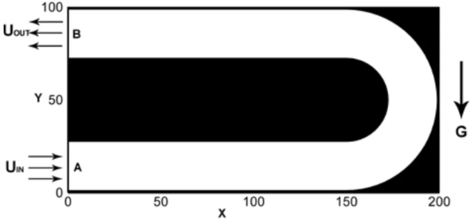
The FH, MLS, and our newly refined mass conserving BC were all designed for a curved boundary, so we tested our new boundary condition for steady flow in a curved pipe, which is very common in practical thermal fluid systems. As shown in Figure 3.1, the fluid flows into the pipe through cross section A and flows out though cross section B. A body force in the form of gravity is applied on the fluid along the negative y-direction.
Figure 3.1: Schematic computational area for flow in a curved pipe
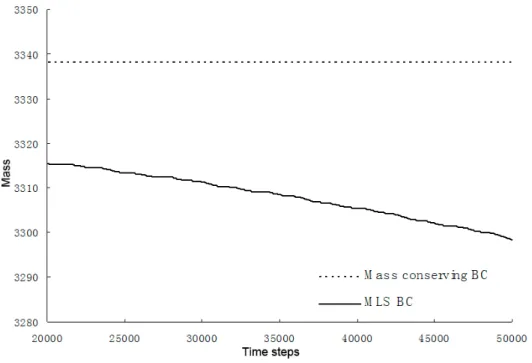
On the wall of the pipe, equations (2.2)-(2.7) are used to update the boundary conditions for the ~f(xb,t)functions. Figure 3.2 shows the resulting x-velocity and y-velocity contours using the mass conserving B
C, respectively. Figure 3.3 shows how the total system mass changes with time. Our new boundary condition can cause the total system mass to converge to a constant value, while the MLS BC demonstrates a steady mass leakage.
a
b
Figure 3.3: System mass change with time using the mass conserving BC and MLS BC
3.2 STEADY AND UNSTEADY FLOW OVER A CIRCULAR CYLINDER
ity of avoiding constant mass leakage. To further ex ine the accuracy of the mass conserving BC method on a curved wall, we conducted a final set of tests concerns 2-D steady and unsteady flows around a circular cylinder placed in a rectangular channel. For steady-state flow, the problem at Re=10 is tested. For unsteady flow, the simulation is at Re=100, resulting in a periodical vortex sheet.
As shown in Figure 3.4, for steady-state problems, the circular cylinder is placed in a domain with nodes, and the center of the cylinder is at the origin (0, 0) of the grids. The
From the tests in Section 3.1, our mass conserving BC shows the expected abil am
70 105
periodical boundary condition treatment is used for the upper and lower boundaries. A uniform velocity is used at the inlet, and the extrapolation boundary condition is used at the outlet.
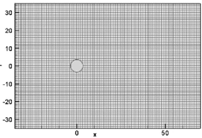
Figure 3.4: Schematic of the computational area for steady flow over a circular cylinder. The cylinder has a diameter of 7 lattice units. The cylinder center-to-center distance (H) is 70
On the surface of the circular cylinder, the mass conserving BC treatment is used to update the bounda
lattice units
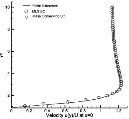
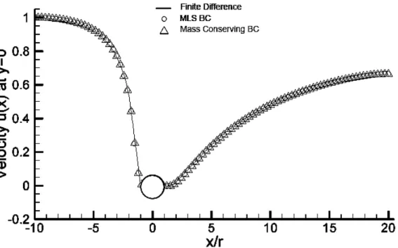
ry conditions for the ~f(xb,t)values. Figure 3.5 shows the streamline and the contour of the pressure at Re2Vr/ 10using a radius (r) of 3.5. Figure 3.6 shows the velocity profile
V y x
u( 0, )/ for H/r20 at Re10. The MLS BC was also used in the same conditions and grids for comparison. The finite difference solution is obtained using body-fitted coordinates and are distributed along the upper surface of the circle over 200 grid points. Figure 3.7 shows the centerline (y=0) velocity variations, upstream and downstream, at Re=10. The results using the MLS BC and finite different results are also presented for comparison.
difference in the results between the MLS and mass conserving BC is around 0.01% of the MLS BC’s results (this difference cannot clearly be seen from the figures). Hence, our mass conserving BC would not reduce the accuracy for problems with geometries that include curved geometry boundaries.
Figure 3.5: Steady flow around a cylinder at Re=10, with streamlines and pressure contours
Figure 3.6: Comparison of the velocity profiles at x=0 for the MLS BC, mass conserving BC and finite difference result for Re=10
Figure 3.7: Comparison of the velocity variation at the centerline (y=0) for the MLS BC, mass conserving BC and finite difference result for Re=10
For unsteady flow, the problem is tested in a 300100 node regime, with a radius of r=6. The periodical boundary condition treatment is used for the upper and lower boundaries. Again, m velocity is given at the inlet, and the extrapolation boundary condition is used at the outlet. The results of the developed periodical flow are shown in Figure 3.8 for the x-velocity and y-velocity contours, respectively. Our mass conserving BC shows necessary capacity of describing and predicting unsteady flow problems. Like other curved BCs, such as FH and MLS, our BC does not cause obvious jagged velocity and pressure distribution near the solid boundary wall in this low grid resolution case (the radius of the cylinder is only 6 grids).
a
b
Figure 3.8: Unsteady flow around a cylinder at Re=100: (a) x-velocity contour; (b) y-velocity contour
3.3 CONCLUSION AND DISCUSSION
In summary, we have proposed a second-order accurate mass conserving boundary condition for the LBE method. Our mass conserving BC will not result in the constant mass
leakage that occurs for other both first- and second-order BCs in some cases. We can derive an expression for the mass leakage of the MLS BC, which can be calculated by:
g ny erval time nx leakage mass 0.5*( 1)* int *[( 1)(1)] (3.1) This shows that the larger the gravity or body force, the larger the mass leakage, so our BC is a good alternative for solving problems with large magnitudes of body forces, such as gravity or a magnetic force.
Moreover, when there is the presence of an “artificial gravity” for certain problems, such as a thermal problem with natural convection, there are also benefits from using our mass conserving BC. For example, the Rayleigh number, which is important in many thermal-fluid problems, is defined as
3 ny T gRa , where is the thermal expansion coefficient, and is the lattice size in the y direction. Hence, in such problems, when we want to simulate a large Rayleigh number, we can increase the gravity instead of using more grid units in the y-direction, because increasing gravity does not significantly add to the computation load. By doing so, the efficiency of the code can be obviously increased when a relatively larger Rayleigh number is needed. Although increasing the grids in the y-direction may seem more direct and efficient, because it is a cubic in the equation, the increasing of grids can lead to a large increase in computational time and money for many cases.
Additionally, because each lattice must be square or cubic (for a 3D problem), to
maintain the ratio so need to also increase
and . The Rayleigh number commonly ranges from to for practical engineering ble
ny
in the simulation domain, when ny is increased, we al
nx pro nz m 3 10 10 8
s. Hence, adjusting the Rayleigh number by only changing ny would make the simulation very inefficient. Furthermore, the amount of available physical memory and the
operating system’s addressing capability [33] strictly limits the number of grids. For three-dimensional problems, especially for multi-component, multi-phase flows or a thermal system, the memory usage often reaches that limit. When using the MLS BC lso ses the mass leakage, as seen in equation (3.1). Since our BC allows the requirement of mass c
system. In the flowing chapters, we will introduce more practical applica
, increasing the grids a increa
onservation to be exactly met, the stability of the model is greatly increased. With this accurate and stable BC treatment, LBE method can be used at more practical problems such as multi-component multi-phase
4.0 THE LBE METHOD FOR MULTI-COMPONENT MULTI-PHASE FLOW WITH HIGH DENSITY RATIOS
odels and mesoscopic kinetic equations, it offers many advantages for the study of multi-component or multi-phase flow problems. While the original formulation of Shan and Chen’s (SC) model can incorporate some multiple phase and component scenarios, the density ratio of the different components is greatly restricted (less than approximately 2.0). This obviously limits the applications of this MCMP LBE model. Hence, based on the original SC MCMP model and the improvements in the single-component multi-phase (SCMP) flow model reported by Yuan and Schaefer [19], we have developed a new model that can simulate a MCMP system with a high density ratio.
4.1 INTRODUCTION TO MCMP FLOW WITH HIGH DENSITY RATIOS
As in the single component multi-phase flow case, the separation of different components in MCMP flows is also due to the long-range interaction between the molecules of the fluid [18], so the interaction force must be revised to also include two parts for a multi-component fluid. One contribution is the interaction between molecules of the same component, and another is the Multi-component multi-phase (MCMP) flow is very common in engineering or industrial problems and in nature. Because the lattice Boltzmann equation (LBE) model is based on microscopic m
interaction between molecules from different components. In a similar manner as in equation (1.13), these two parts can be expressed as:
x g
x c x Fi,i() 0i iii (4.1)
x
c x Fi,j() 0i gij j x
i j (4.2) i iF, is the force between the different particles of component , and i Fi,j indicates the ponent and component
force between the com i j.
To increase the density ratio between different components, one first should increase the density ratio for the different phases of each single component. Work has already been done on increasing the density ratio for single-component multi-phase (SCMP) flows. For example, as reported by Swift [ 34 ], the maximum density ratio obtained using the free-energy-based approach is less than 10:1, and the largest density ratio tested in the He, Chen and Zhang (HCZ) approach is 40:1 [35]. These are improvements, but are still not large enough for most practical problems. This is because the idea gas EOS and original SC model show unrealistic pressure-density relationship. They give a high compressibility for the liquid phase, which is even higher than the vapor phase. Yuan and Schaefer [19] found, hence, that is possible to simulate SCMP flows with a density ratio that can reach 1,000:1 by using a more accurate EOS such as the van der Waals, Peng-Robinson, or Carnahan-Starling EOS [36], and all of these EOSs are easy to .21) apply to the LBE model. To do so, first, the pressure term in equation (1
(
g c0 c p s2 2 ) ( ) is replaced by the pressure formulation in an EOS (using Peng-Robinson
as example, 2 2 2 ) ( RT a T
P ). Secondly, the effective mass is substituted into 2
1
x Ftotal i i eq u u i i ,equation (1.20) is used to calculate the shifted velocity (
). Achieving a
density ratio of up to 1,000:1 mean most single-component vapor-liquid flows.
Unlike in the original SC model, though, the coefficient of interaction strength within a component
.1) and (4.2). The only requirement for is to ensu
important for creating and extending the MCMP LBE model. Firstly, when equation ) is substituted tion (4.2), is not eliminated. Secondly, from equation (4.2
4.2 SIMULATION OF AN EQUILIBRIUM DROPLET WITHOUT A BODY FORCE
The first example is the simulation of a circular droplet in a
s that the LBE model can work well for the simulation of
(g ) here cannot control the overall interaction strength. (Indeed, it is canceled out when we substitute equation (1.21) into equation (4
ii into equa ii g (1.21 ), it can be re that the whole term inside the square root in equation (1.21) is positive. However, we have found that the coefficient of interaction strength between different components is very
ij
seen that gij affects the magnitude of the interparticle force between different components Fi,j. The behavior of the interaction between the different components is primarily controlled by this force, so interaction can be adjusted through changing the value of gij. From our tests, this force plays a critical role in adjusting the system density ratio, which we will explain and demonstrate in the following sections.
AND EXTERNAL FORCES
ij g g 100 100 d 2D square domain boundary con ition is appl
two vertical boundaries (x0 and x100
and 100
), and a bounce back treatment is used for the upper and bottom boundaries (y0 y ). For an initial condition for component 1 (the liquid component), we specified a low density value ( 0.005) for most of the simulation region, except for a circular area at the center of the sim lation space, where a high density value was set (
u 1
). For component 2 (the gas component), density was set to a relatively higher 01
. 0
) at most areas of the sim lation domain, except the center u value than component 1 (
circle area (corresponding to the liquid component), where an extremely low density was used ( 0.0001). Generally, if the problem can reach a converged result, the shape of the high density area is not important. A square, triangle, or any random geometry will not affect the final result. Because a droplet always tends to become the shape that has smallest surface area, for this 2D case, the droplet will alway become a circle. Hence, setting the initial shape to a circle increases the problem’s convergence speed, since as with most numerical methods, the less difference between the initial conditions and final result, the faster the model converges.
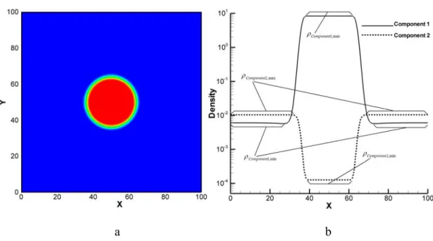
s
ce, p m dens
Figure 4.1a shows the density contour of component 1 (the liquid component), and Figure 4.1b shows the comparison of the density of the two components along the center line (y50, 0 x100) on a log scale. For convenien10
density of com u we have onent 1, m hi i ghlight nimum p
nt 2, and minim ity of component 2, noted as ed several segm density of com
ents on these lines, which onent 1, maximum density
max , 1 are the m of com aximum
pone Component , Component1,min,
max , 2 Component
, and Component2,min, respectively. The density variation in each segment is very small compared to the density change at the interface of the different components, so this sm
p
all onent 1 in the droplet variation can be neglected. In Figure 4.1b, the density of com
(Component2,max) is on the order of ence the density ratio of these two components is around 1,000. In general, the density ratio of a system refers to the ratio between the maximum
2
10 . H
densities of the two components (
max , 2 max , 1 Component Component ). a b
Figure 4.1: (a) Density contour for a circular droplet, (b) Comparison of the densities of the two components along the center line (y50, 0x100
Maximum Force Ratio
)
in Section 4.1, the balance of the weights of the two parts and 4.2.1
As detailed Fi,i Fi,j
directly affects the density ratio of the different components. The forces Fi,i and vary in the ain and reach a m m value around th
Figure 4.2 shows the distribution of the ratio of and in the test area, wh
j i
F,
ere
simulation dom aximu e interface of the two components.
x
is
x