January 2013, Volume 52, Issue 5. http://www.jstatsoft.org/
Fast and Elegant Numerical Linear Algebra Using
the
RcppEigen
Package
Douglas Bates
University of Wisconsin-Madison
Dirk Eddelbuettel
Debian Project
Abstract
The RcppEigen package provides access from R (RCore Team 2012a) to the Eigen
(Guennebaud, Jacob, and others 2012)C++ template library for numerical linear
alge-bra. Rcpp(Eddelbuettel and Fran¸cois 2011,2012) classes and specializations of theC++
templated functions asand wrapfrom Rcppprovide the “glue” for passing objects from
RtoC++and back. Several introductory examples are presented. This is followed by an
depth discussion of various available approaches for solving least-squares problems, in-cluding rank-revealing methods, conin-cluding with an empirical run-time comparison. Last but not least, sparse matrix methods are discussed.
Keywords: linear algebra, template programming, R,C++,Rcpp.
1. Introduction
Linear algebra is an essential building block of statistical computing. Operations such as matrix decompositions, linear program solvers, and eigenvalue/eigenvector computations are used in many estimation and analysis routines. As such, libraries supporting linear algebra have long been provided by statistical programmers for different programming languages and environments. Because it is object-oriented, C++, one of the central modern languages for numerical and statistical computing, is particularly effective at representing matrices, vectors and decompositions, and numerous class libraries providing linear algebra routines have been written over the years.
As both theC++language and standards have evolved (Meyers 2005,1995;ISO/IEC 2011), so have the compilers implementing the language. Relatively modern language constructs such as template meta-programming are particularly useful because they provide overloading of operations (allowing expressive code in the compiled language similar to what can be done in scripting languages) and can shift some of the computational burden from the run-time to the
compile-time. (A more detailed discussion of template meta-programming is, however, beyond the scope of this paper). Veldhuizen(1998) provided an early and influential implementation of numerical linear algebra classes that already demonstrated key features of this approach. Its usage was held back at the time by the limited availability of compilers implementing all the necessary features of theC++ language.
This situation has greatly improved over the last decade, and many more libraries have been made available. One such C++ library is Eigen by Guennebaud, Jacob, and others (2012) which started as a sub-project to KDE (a popular Linux desktop environment), initially focussing on fixed-size matrices to represent projections in a visualization application. Eigen
grew from there and has over the course of about a decade produced three major releases withEigen3 being the current major version. To check the minor and patch version numbers, load the RcppEigen package and call
R> .Call("eigen_version", FALSE)
major minor patch
3 1 1
Eigen is of interest as the Rsystem for statistical computation and graphics (R Core Team 2012a) is itself easily extensible. This is particular true via the C language that most of R’s compiled core parts are written in, but also for the C++ language which can interface with C-based systems rather easily. The manual “Writing R Extensions” (R Core Team 2012b) is the basic reference for extending Rwith either C orC++.
The Rcpp package byEddelbuettel and Fran¸cois (2011,2012), see alsoEddelbuettel (2013), facilitates extending Rwith C++ code by providing seamless object mapping between both languages. As stated in the Rcppvignette, “Extending Rcpp”
Rcpp facilitates data interchange between R and C++ through the templated functions Rcpp::as (for conversion of objects from R to C++) and Rcpp::wrap
(for conversion from C++toR).
TheRcppEigenpackage provides the header files composing theEigenC++template library, along with implementations of Rcpp::as and Rcpp::wrap for the C++ classes defined in
Eigen.
The Eigen classes themselves provide high-performance, versatile and comprehensive repre-sentations of dense and sparse matrices and vectors, as well as decompositions and other functions to be applied to these objects. The next section introduces some of these classes and shows how to interface to them from R.
2.
Eigen
classes
Eigenis aC++template library providing classes for many forms of matrices, vectors, arrays and decompositions. These classes are flexible and comprehensive allowing for both high performance and well structured code representing high-level operations. C++code based on
Eigen is often more like R code, working on the “whole object”, than like compiled code in other languages where operations often must be coded in loops.
Robject type Eigen class typedef
numeric matrix MatrixXd
integer matrix MatrixXi
complex matrix MatrixXcd
numeric vector VectorXd
integer vector VectorXi
complex vector VectorXcd
Matrix::dgCMatrix SparseMatrix<double>
Table 1: Correspondence betweenRmatrix and vector types and classes in theEigen names-pace.
As in manyC++template libraries using template meta-programming (Abrahams and Gur-tovoy 2004), the templates themselves can be very complicated. However, Eigen provides
typedefs for common classes that correspond toRmatrices and vectors, as shown in Table1, and this paper will use these typedefs.
Here, Vector and Matrix describe the dimension of the object. The X signals that these are dynamically-sized objects (as opposed to fixed-size matrices such as 3×3 matrices also available inEigen). Lastly, the trailing characters i, dand cd denote, respectively, storage types integer,double andcomplex double.
The C++classes shown in Table1are in theEigen namespace, which means that they must be written as Eigen::MatrixXd. However, if one prefaces the use of these class names with a declaration like
using Eigen::MatrixXd;
then one can use these names without the namespace qualifier.
2.1. Mapped matrices in Eigen
Storage for the contents of matrices from the classes shown in Table 1 is allocated and con-trolled by the class constructors and destructors. Creating an instance of such a class from an Robject involves copying its contents. An alternative is to have the contents of the Rmatrix or vector mapped to the contents of the object from the Eigen class. For dense matrices one can use the Eigentemplated classMap, and for sparse matrices one can deploy the Eigen
templated class MappedSparseMatrix.
One must, of course, be careful not to modify the contents of theRobject in the C++code. A recommended practice is always to declare mapped objects as const.
2.2. Arrays in Eigen
For matrix and vector classes Eigen overloads the ‘*’ operator as matrix multiplication. Occasionally component-wise operations instead of matrix operations are desired, for which theArraytemplated classes are used inEigen. Switching back and forth between matrices or vectors and arrays is usually done via the array()method for matrix or vector objects and thematrix()method for arrays.
2.3. Structured matrices in Eigen
Eigenprovides classes for matrices with special structure such as symmetric matrices, triangu-lar matrices and banded matrices. For dense matrices, these special structures are described as “views”, meaning that the full dense matrix is stored but only part of the matrix is used in operations. For a symmetric matrix one must specify whether the lower triangle or the upper triangle is to be used as the contents, with the other triangle defined by the implicit symmetry.
3. Some simple examples
C++functions to perform simple operations on matrices or vectors can follow a pattern of: 1. Map theRobjects passed as arguments into Eigen objects.
2. Create the result.
3. ReturnRcpp::wrapapplied to the result. An idiom for the first step is
using Eigen::Map;
using Eigen::MatrixXd;
using Rcpp::as;
const Map<MatrixXd> A(as<Map<MatrixXd> >(AA));
where AA is the name of the R object (of type SEXP in C and C++) passed to the C++ function.
An alternative to theusing declarations is to declare atypedefas in
typedef Eigen::Map<Eigen::MatrixXd> MapMatd;
const MapMatd A(Rcpp::as<MapMatd>(AA));
The cxxfunction function from the inline package (Sklyar, Murdoch, Smith, Eddelbuettel, and Fran¸cois 2012) forRand itsRcppEigenplugin provide a convenient method of developing and debugging theC++code. For actual production code one generally incorporates theC++ source code files in a package and includes the line LinkingTo: Rcpp, RcppEigen in the package’s DESCRIPTION file. The RcppEigen.package.skeleton function provides a quick way of generating the skeleton of a package that will useRcppEigen.
The cxxfunction with the "Rcpp" or "RcppEigen" plugins has the as and wrap functions already defined asRcpp::as and Rcpp::wrap. In the examples below these declarations are omitted. It is important to remember that they are needed in actualC++ source code for a package.
The first few examples are simply for illustration as the operations shown could be more effectively performed directly in R. Finally, the results from Eigen are compared to those from the directRresults.
using Eigen::Map;
using Eigen::MatrixXi;
// Map the integer matrix AA from R
const Map<MatrixXi> A(as<Map<MatrixXi> >(AA));
// evaluate and return the transpose of A
const MatrixXi At(A.transpose());
return wrap(At);
Figure 1: transCpp: Transpose a matrix of integers.
3.1. Transpose of an integer matrix
The nextRcode snippet creates a simple matrix of integers R> (A <- matrix(1:6, ncol = 2)) [,1] [,2] [1,] 1 4 [2,] 2 5 [3,] 3 6 R> str(A) int [1:3, 1:2] 1 2 3 4 5 6
and, in Figure 1, the transpose() method for the Eigen::MatrixXi class is used to re-turn the transpose of the supplied matrix. The R matrix in the SEXP AA is first mapped to an Eigen::MatrixXi object, and then the matrix At is constructed from its transpose and returned toR.
The R snippet below compiles and links the C++ code segment. The actual work is done by the function cxxfunction from the inline package which compiles, links and loads code written in C++ and supplied as a character variable. This frees the user from having to know about compiler and linker details and options, which makes “exploratory programming” much easier. Here the program piece to be compiled is stored as a character variable named
transCpp, and cxxfunction creates an executable function which is assigned to ftrans. This new function is used on the matrixA shown above, and one can check that it works as intended by comparing the output to an explicit transpose of the matrix argument.
R> ftrans <- cxxfunction(signature(AA = "matrix"), transCpp, + plugin = "RcppEigen") R> (At <- ftrans(A)) [,1] [,2] [,3] [1,] 1 2 3 [2,] 4 5 6 R> stopifnot(all.equal(At, t(A)))
typedef Eigen::Map<Eigen::MatrixXi> MapMati;
const MapMati B(as<MapMati>(BB));
const MapMati C(as<MapMati>(CC));
return List::create(Named("B %*% C") = B * C,
Named("crossprod(B, C)") = B.adjoint() * C);
Figure 2: prodCpp: Product and cross-product of two matrices.
For numeric or integer matrices the adjoint() method is equivalent to the transpose()
method. For complex matrices, the adjoint is the conjugate of the transpose. In keeping with the conventions in the Eigen documentation the adjoint() method is used in what follows to create the transpose of numeric or integer matrices.
3.2. Products and cross-products
As mentioned in Section2.2, the‘*’ operator is overloaded as matrix multiplication for the various matrix and vector classes inEigen. TheC++code in Figure2produces a list contain-ing both the product and cross-product (in the sense of theRfunction callcrossproduct(A, B)evaluating A>B) of its two arguments
R> fprod <- cxxfunction(signature(BB = "matrix", CC = "matrix"), + prodCpp, "RcppEigen") R> B <- matrix(1:4, ncol = 2) R> C <- matrix(6:1, nrow = 2) R> str(fp <- fprod(B, C)) List of 2 $ B %*% C : int [1:2, 1:3] 21 32 13 20 5 8 $ crossprod(B, C): int [1:2, 1:3] 16 38 10 24 4 10
R> stopifnot(all.equal(fp[[1]], B %*% C), all.equal(fp[[2]], crossprod(B, C))) Note that the create class method for Rcpp::List implicitly applies Rcpp::wrap to its arguments.
3.3. Crossproduct of a single matrix
As shown in the last example, theRfunctioncrossprodcalculates the product of the trans-pose of its first argument with its second argument. The single argument form,crossprod(X), evaluatesX>X. One could, of course, calculate this product as
t(X) %*% X
butcrossprod(X)is roughly twice as fast because the result is known to be symmetric and only one triangle needs to be calculated. The functiontcrossprodevaluatescrossprod(t(X))
using Eigen::Map;
using Eigen::MatrixXi;
using Eigen::Lower;
const Map<MatrixXi> A(as<Map<MatrixXi> >(AA));
const int m(A.rows()), n(A.cols()); MatrixXi AtA(MatrixXi(n, n).setZero().
selfadjointView<Lower>().rankUpdate(A.adjoint())); MatrixXi AAt(MatrixXi(m, m).setZero().
selfadjointView<Lower>().rankUpdate(A));
return List::create(Named("crossprod(A)") = AtA, Named("tcrossprod(A)") = AAt);
Figure 3: crossprodCpp: Cross-product and transposed cross-product of a single matrix.
To express these calculations inEigen, aSelfAdjointView—which is a dense matrix of which only one triangle is used, the other triangle being inferred from the symmetry—is created. (The characterization “self-adjoint” is equivalent to symmetric for non-complex matrices.) TheEigen class name is SelfAdjointView. The method for general matrices that produces such a view is called selfadjointView. Both require specification of either the Lower or
Uppertriangle.
For triangular matrices the class is TriangularView and the method is triangularView. The triangle can be specified as Lower, UnitLower, StrictlyLower, Upper, UnitUpper or
StrictlyUpper.
For self-adjoint views therankUpdatemethod adds a scalar multiple of AA> to the current symmetric matrix. The scalar multiple defaults to 1. The code in Figure 3 produces both A>A and AA> from a matrix A.
R> fcprd <- cxxfunction(signature(AA = "matrix"), crossprodCpp, "RcppEigen") R> str(crp <- fcprd(A)) List of 2 $ crossprod(A) : int [1:2, 1:2] 14 32 32 77 $ tcrossprod(A): int [1:3, 1:3] 17 22 27 22 29 36 27 36 45 R> stopifnot(all.equal(crp[[1]], crossprod(A)), + all.equal(crp[[2]], tcrossprod(A)))
To some, the expressions in Figure 3 to constructAtAand AAt are compact and elegant. To others they are hopelessly confusing. If you find yourself in the latter group, you just need to read the expression left to right. So, for example, we construct AAtby creating a general integer matrix of size m×m (where A is m×n), ensuring that all its elements are zero, regarding it as a self-adjoint (i.e., symmetric) matrix using the elements in the lower triangle, then adding AA> to it and converting back to a general matrix form (i.e., the strict lower triangle is copied into the strict upper triangle).
using Eigen::LLT; using Eigen::Lower; using Eigen::Map; using Eigen::MatrixXd; using Eigen::MatrixXi; using Eigen::Upper; using Eigen::VectorXd;
typedef Map<MatrixXd> MapMatd;
typedef Map<MatrixXi> MapMati;
typedef Map<VectorXd> MapVecd;
inline MatrixXd AtA(const MapMatd& A) {
int n(A.cols());
return MatrixXd(n,n).setZero().selfadjointView<Lower>() .rankUpdate(A.adjoint());
}
Figure 4: The contents of the character vector, incl, that will preface C++ code segments that follow.
1. MatrixXi(n, n) creates ann×ninteger matrix with arbitrary contents 2. .setZero() zeros out the contents of the matrix
3. .selfAdjointView<Lower>() causes what follows to treat the matrix as a symmetric matrix in which only the lower triangle is used, the strict upper triangle being inferred by symmetry
4. .rankUpdate(A) forms the sumB+AA> where B is the symmetric matrix of zeros created in the previous steps.
The assignment of this symmetric matrix to the (general) MatrixXi object AAt causes the result to be symmetrized during the assignment.
For these products one could define the symmetric matrix from either the lower triangle or the upper triangle as the result will be symmetrized before it is returned.
To cut down on repetition ofusingstatements we gather them in a character variable,incl, that will be given as the includesargument in the calls to cxxfunction. We also define a utility function,AtA, that returns the crossproduct matrix as shown in Figure4
3.4. Cholesky decomposition of the crossprod
The Cholesky decomposition of the positive-definite, symmetric matrix,A, can be written in several forms. Numerical analysts define the “LLt” form as the lower triangular matrix, L, such thatA=LL>and the “LDLt” form as a unit lower triangular matrixLand a diagonal matrix D with positive diagonal elements such that A = LDL>. Statisticians often write the decomposition asA=R>R whereRis an upper triangular matrix. Of course, this Ris simply the transpose of L from the “LLt” form.
const LLT<MatrixXd> llt(AtA(as<MapMatd>(AA)));
return List::create(Named("L") = MatrixXd(llt.matrixL()), Named("R") = MatrixXd(llt.matrixU()));
Figure 5: cholCpp: Cholesky decomposition of a cross-product.
The templatedEigenclasses for the LLt and LDLt forms are calledLLTandLDLTand the cor-responding methods are.llt() and .ldlt(). Because the Cholesky decomposition involves taking square roots, we pass a numeric matrix,A, not an integer matrix.
R> storage.mode(A) <- "double"
R> fchol <- cxxfunction(signature(AA = "matrix"), cholCpp, "RcppEigen", incl) R> (ll <- fchol(A)) $L [,1] [,2] [1,] 3.74166 0.00000 [2,] 8.55236 1.96396 $R [,1] [,2] [1,] 3.74166 8.55236 [2,] 0.00000 1.96396 R> stopifnot(all.equal(ll[[2]], chol(crossprod(A))))
3.5. Determinant of the cross-product matrix
The “D-optimal” criterion for experimental design chooses the design that maximizes the determinant, |X>X|, for then×pmodel matrix (or Jacobian matrix),X. The determinant, |L|, of thep×plower Cholesky factorL, defined so thatLL>=X>X, is the product of its diagonal elements, as is the case for any triangular matrix. By the properties of determinants,
|X>X|=|LL>|=|L| |L>|=|L|2
Alternatively, if using the “LDLt” decomposition, LDL> = X>X where L is unit lower triangular and D is diagonal then |X>X| is the product of the diagonal elements of D. Because it is known that the diagonal elements ofDmust be non-negative, one often evaluates the logarithm of the determinant as the sum of the logarithms of the diagonal elements of D. Several options are shown in Figure 6.
R> fdet <- cxxfunction(signature(AA = "matrix"), cholDetCpp, "RcppEigen", + incl)
R> unlist(ll <- fdet(A))
d1 d2 ld 54.00000 54.00000 3.98898
const MatrixXd ata(AtA(as<MapMatd>(AA)));
const double detL(MatrixXd(ata.llt().matrixL()).diagonal().prod());
const VectorXd Dvec(ata.ldlt().vectorD());
return List::create(Named("d1") = detL * detL, Named("d2") = Dvec.prod(),
Named("ld") = Dvec.array().log().sum());
Figure 6: cholDetCpp: Determinant of a cross-product using the “LLt” and “LDLt” forms of the Cholesky decomposition.
Note the use of thearray() method in the calculation of the log-determinant. Because the
log() method applies to arrays, not to vectors or matrices, an array must be created from
Dvecbefore applying thelog() method.
4. Least squares solutions
A common operation in statistical computing is calculating a least squares solution,β, definedb as
b
β= argmin β
ky−Xβk2
where the model matrix,X, isn×p(n≥p) andyis ann-dimensional response vector. There are several ways, based on matrix decompositions, to determine such a solution. Earlier, two forms of the Cholesky decomposition were discussed: “LLt” and “LDLt”, which can both be used to solve for β. Other decompositions that can be used are the QR decomposition, withb or without column pivoting, the singular value decomposition and the eigendecomposition of a symmetric matrix.
Determining a least squares solution is relatively straightforward. However, statistical com-puting often requires additional information, such as the standard errors of the coefficient estimates. Calculating these involves evaluating the diagonal elements of X>X−1
and the residual sum of squares, ky−Xβkb 2.
4.1. Least squares using the “LLt” Cholesky
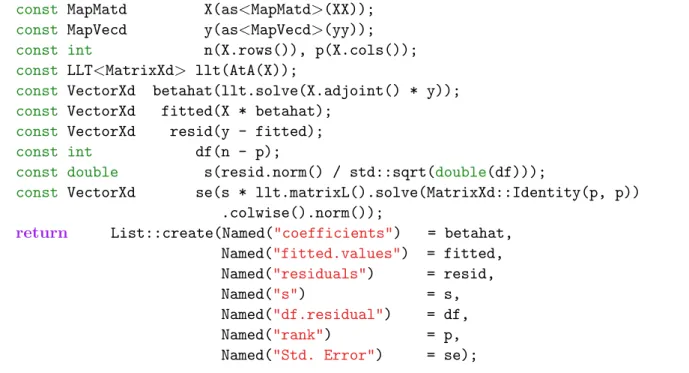
Figure 7 shows a calculation of the least squares coefficient estimates (betahat) and the standard errors (se) through an “LLt” Cholesky decomposition of the crossproduct of the model matrix, X. Next, the results from this calculation are compared to those from the
lm.fit function inR(lm.fit is the workhorse function called bylm once the model matrix and response have been evaluated).
R> lltLS <- cxxfunction(signature(XX = "matrix", yy = "numeric"), lltLSCpp, + "RcppEigen", incl)
R> data("trees", package = "datasets")
R> str(lltFit <- with(trees, lltLS(cbind(1, log(Girth)), log(Volume))))
List of 7
const MapMatd X(as<MapMatd>(XX));
const MapVecd y(as<MapVecd>(yy));
const int n(X.rows()), p(X.cols());
const LLT<MatrixXd> llt(AtA(X));
const VectorXd betahat(llt.solve(X.adjoint() * y));
const VectorXd fitted(X * betahat);
const VectorXd resid(y - fitted);
const int df(n - p);
const double s(resid.norm() / std::sqrt(double(df)));
const VectorXd se(s * llt.matrixL().solve(MatrixXd::Identity(p, p)) .colwise().norm());
return List::create(Named("coefficients") = betahat, Named("fitted.values") = fitted, Named("residuals") = resid, Named("s") = s, Named("df.residual") = df, Named("rank") = p, Named("Std. Error") = se);
Figure 7: lltLSCpp: Least squares using the Cholesky decomposition.
$ fitted.values: num [1:31] 2.3 2.38 2.43 2.82 2.86 ... $ residuals : num [1:31] 0.0298 -0.0483 -0.1087 -0.0223 0.0727 ... $ s : num 0.115 $ df.residual : int 29 $ rank : int 2 $ Std. Error : num [1:2] 0.2307 0.0898
R> str(lmFit <- with(trees, lm.fit(cbind(1, log(Girth)), log(Volume)))) List of 8
$ coefficients : Named num [1:2] -2.35 2.2 ..- attr(*, "names")= chr [1:2] "x1" "x2"
$ residuals : num [1:31] 0.0298 -0.0483 -0.1087 -0.0223 0.0727 ...
$ effects : Named num [1:31] -18.2218 2.8152 -0.1029 -0.0223 0.0721 ... ..- attr(*, "names")= chr [1:31] "x1" "x2" "" "" ... $ rank : int 2 $ fitted.values: num [1:31] 2.3 2.38 2.43 2.82 2.86 ... $ assign : NULL $ qr :List of 5 ..$ qr : num [1:31, 1:2] -5.57 0.18 0.18 0.18 0.18 ... ..$ qraux: num [1:2] 1.18 1.26 ..$ pivot: int [1:2] 1 2 ..$ tol : num 1e-07 ..$ rank : int 2
..- attr(*, "class")= chr "qr" $ df.residual : int 29
R> for(nm in c("coefficients", "residuals", "fitted.values", "rank")) + stopifnot(all.equal(lltFit[[nm]], unname(lmFit[[nm]])))
R> stopifnot(all.equal(lltFit[["Std. Error"]],
+ unname(coef(summary(lm(log(Volume) ~ log(Girth), trees)))[,2])))
There are several aspects of theC++code in Figure7worth mentioning. Thesolvemethod for theLLTobject evaluates, in this case, X>X−1
X>ybut without actually evaluating the inverse. The calculation of the residuals,y−y, can be written, as inb R, asy - fitted. (But note thatEigenclasses do not have a “recycling rule” as inR. That is, the two vector operands must have the same length.) The norm() method evaluates the square root of the sum of squares of the elements of a vector. Although one does not explicitly evaluate X>X−1 one does evaluate L−1 to obtain the standard errors. Note also the use of thecolwise()method in the evaluation of the standard errors. It applies a method to the columns of a matrix, returning a vector. TheEigencolwise()androwwise() methods are similar in effect to the
apply function inR.
In the descriptions of other methods for solving least squares problems, much of the code parallels that shown in Figure 7. The redundant parts are omitted, and only the evaluation of the coefficients, the rank and the standard errors is shown. Actually, the standard errors are calculated only up to the scalar multiple of s, the residual standard error, in these code fragments. The calculation of the residuals and s and the scaling of the coefficient standard errors is the same for all methods. (See the filesfastLm.hand fastLm.cppin theRcppEigen
source package for details.)
4.2. Least squares using the unpivoted QR decomposition
A QR decomposition has the form
X =QR=Q1R1
whereQ is ann×northogonal matrix, which means thatQ>Q=QQ> =In, and then×p
matrix R is zero below the main diagonal. The n×p matrix Q1 is the first p columns of Q and the p×p upper triangular matrixR1 is the top p rows ofR. There are three Eigen classes for the QR decomposition: HouseholderQR provides the basic QR decomposition using Householder transformations, ColPivHouseholderQR incorporates column pivots and
FullPivHouseholderQRincorporates both row and column pivots.
Figure 8 shows a least squares solution using the unpivoted QR decomposition. The calcu-lations in Figure 8 are quite similar to those in Figure 7. In fact, if one had extracted the upper triangular factor (thematrixU()method) from the LLTobject in Figure7, the rest of the code would be nearly identical.
4.3. Handling the rank-deficient case
One important consideration when determining least squares solutions is whether rank(X) is p, a situation described by saying thatX has “full column rank”. WhenX does not have full column rank it is said to be “rank deficient”.
Although the theoretical rank of a matrix is well-defined, its evaluation in practice is not. At best one can compute an effective rank according to some tolerance. Decompositions that allow to estimation of the rank of the matrix in this way are said to be “rank-revealing”.
using Eigen::HouseholderQR;
const HouseholderQR<MatrixXd> QR(X);
const VectorXd betahat(QR.solve(y));
const VectorXd fitted(X * betahat);
const int df(n - p);
const VectorXd se(QR.matrixQR().topRows(p).triangularView<Upper>() .solve(MatrixXd::Identity(p,p)).rowwise().norm());
Figure 8: QRLSCpp: Least squares using the unpivoted QR decomposition.
Because the model.matrix function in R does a considerable amount of symbolic analysis behind the scenes, one usually ends up with full-rank model matrices. The common cases of rank-deficiency, such as incorporating both a constant term and a full set of indicators columns for the levels of a factor, are eliminated. Other, more subtle, situations will not be detected at this stage, however. A simple example occurs when there is a “missing cell” in a two-way layout and the interaction of the two factors is included in the model.
R> dd <- data.frame(f1 = gl(4, 6, labels = LETTERS[1:4]), + f2 = gl(3, 2, labels = letters[1:3]))[-(7:8), ] R> xtabs(~ f2 + f1, dd) f1 f2 A B C D a 2 0 2 2 b 2 2 2 2 c 2 2 2 2 R> mm <- model.matrix(~ f1 * f2, dd) R> kappa(mm) [1] 4.30923e+16
This yields a large condition number, indicating rank deficiency. Alternatively, the reciprocal condition number can be evaluated.
R> rcond(mm)
[1] 2.3206e-17
R> (c(rank = qr(mm)$rank, p = ncol(mm)))
rank p 11 12
R> set.seed(1)
R> dd$y <- mm %*% seq_len(ncol(mm)) + rnorm(nrow(mm), sd = 0.1) R> fm1 <- lm(y ~ f1 * f2, dd)
R> writeLines(capture.output(print(summary(fm1), + signif.stars = FALSE))[9:22])
Coefficients: (1 not defined because of singularities) Estimate Std. Error t value Pr(>|t|)
(Intercept) 0.9779 0.0582 16.8 3.4e-09 f1B 12.0381 0.0823 146.3 < 2e-16 f1C 3.1172 0.0823 37.9 5.2e-13 f1D 4.0685 0.0823 49.5 2.8e-14 f2b 5.0601 0.0823 61.5 2.6e-15 f2c 5.9976 0.0823 72.9 4.0e-16 f1B:f2b -3.0148 0.1163 -25.9 3.3e-11 f1C:f2b 7.7030 0.1163 66.2 1.2e-15 f1D:f2b 8.9643 0.1163 77.1 < 2e-16 f1B:f2c NA NA NA NA f1C:f2c 10.9613 0.1163 94.2 < 2e-16 f1D:f2c 12.0411 0.1163 103.5 < 2e-16
Thelmfunction for fitting linear models inRuses a rank-revealing form of the QR decompo-sition. When the model matrix is determined to be rank deficient, according to the threshold used inR’sqrfunction, the model matrix is reduced to rank (X) columns by pivoting selected columns (those that are apparently linearly dependent on columns to their left) to the right hand side of the matrix. A solution for this reduced model matrix is determined and the coefficients and standard errors for the redundant columns are flagged as missing.
An alternative approach is to evaluate the “pseudo-inverse” of X from the singular value decomposition (SVD) ofX or the eigendecomposition of X>X. The SVD is of the form
X =U DV>=U1D1V>
whereU is an orthogonaln×nmatrix andU1 is its leftmostp columns,D isn×pand zero off the main diagonal so thatD1 is ap×pdiagonal matrix with non-increasing, non-negative diagonal elements, and V is a p×p orthogonal matrix. The pseudo-inverse of D1, written D+1 is a p×p diagonal matrix whose first r = rank(X) diagonal elements are the inverses of the corresponding diagonal elements of D1 and whose last p−r diagonal elements are zero. The tolerance for determining if an element of the diagonal ofD1 is considered to be (effectively) zero is a multiple of the largest singular value (i.e., the (1,1) element ofD). The pseudo-inverse,X+, of X is defined as
X+ =V D+1U1>.
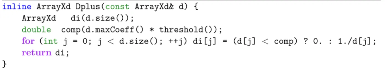
In Figure9a utility function, Dplus, is defined to return the diagonal of the pseudo-inverse, D+1, as an array, given the singular values (the diagonal ofD1) as an array. Calculation of the maximum element of d (the method is called .maxCoeff()) and the use of a threshold()
inline ArrayXd Dplus(const ArrayXd& d) { ArrayXd di(d.size());
double comp(d.maxCoeff() * threshold());
for (int j = 0; j < d.size(); ++j) di[j] = (d[j] < comp) ? 0. : 1./d[j];
return di; }
Figure 9: DplusCpp: Create the diagonal d+ of the pseudo-inverse, D1+, from the array of singular values,d.
X>X, as shown in Section4.5, even though these are returned in increasing order, as opposed to the decreasing order of the singular values.
4.4. Least squares using the SVD
With these definitions the code for least squares using the singular value decomposition can be written as in Figure10. Even in the rank-deficient case this code will produce a complete set of coefficients and their standard errors. The user must be careful to check if the computed rank is less than p, the number of columns in X, in which case the estimated coefficients are just one of an infinite number of coefficient vectors that produce the same fitted values. It happens that the solution from this pseudo-inverse is the minimum norm solution (in the sense thatkβk2 is minimized among those β that minimizeky−Xβk2).
The standard errors of the coefficient estimates in the rank-deficient case must be interpreted carefully. The solution with one or more missing coefficients, as returned by the lm.fit
function in R and by the column-pivoted QR decomposition described in Section 4.6, does not provide standard errors for the missing coefficients. That is, both the coefficient and its standard error are returned asNAbecause the least squares solution is performed on a reduced model matrix. It is also true that the solution returned by the SVD method is with respect to a reduced model matrix but the p coefficient estimates and their p standard errors don’t show this. They are, in fact, linear combinations of a set ofr coefficient estimates and their standard errors.
const Eigen::JacobiSVD<MatrixXd>
UDV(X.jacobiSvd(Eigen::ComputeThinU|Eigen::ComputeThinV));
const ArrayXd Dp(Dplus(UDV.singularValues()));
const int r((Dp > 0).count());
const MatrixXd VDp(UDV.matrixV() * Dp.matrix().asDiagonal());
const VectorXd betahat(VDp * UDV.matrixU().adjoint() * y);
const VectorXd se(s * VDp.rowwise().norm());
const Eigen::SelfAdjointEigenSolver<MatrixXd> VLV(AtA(X));
const ArrayXd Dp(Dplus(eig.eigenvalues()).sqrt());
const int r((Dp > 0).count());
const MatrixXd VDp(VLV.eigenvectors() * Dp.matrix().asDiagonal());
const VectorXd betahat(VDp * VDp.adjoint() * X.adjoint() * y);
const VectorXd se(s * VDp.rowwise().norm());
Figure 11: SymmEigLSCpp: Least squares using the eigendecomposition.
4.5. Least squares using the eigendecomposition
The eigendecomposition ofX>X is defined as
X>X =VΛV>
whereV, the matrix of eigenvectors, is a p×p orthogonal matrix andΛ is a p×p diagonal matrix with non-decreasing, non-negative diagonal elements, called the eigenvalues ofX>X. When the eigenvalues are distinct, thisV is the same (up to reordering of the columns) as that in the SVD and the eigenvalues of X>X are the (reordered) squares of the singular values ofX.
With these definitions one can adapt much of the code from the SVD method for the eigen-decomposition, as shown in Figure11.
4.6. Least squares using the column-pivoted QR decomposition
The column-pivoted QR decomposition provides results similar to those fromR in both the full-rank and the rank-deficient cases. The decomposition is of the form
XP =QR=Q1R1
where, as before,Qis n×n and orthogonal andR isn×p and upper triangular. The p×p matrixP is a permutation matrix. That is, its columns are a permutation of the columns of Ip. It serves to reorder the columns ofX so that the diagonal elements ofRare non-increasing
in magnitude.
An instance of the classEigen::ColPivHouseholderQR has arank() method returning the computational rank of the matrix. When X is of full rank one can use essentially the same code as in the unpivoted decomposition except that one must reorder the standard errors. When X is rank-deficient, the coefficients and standard errors are evaluated for the leading r columns ofXP only.
In the rank-deficient case the straightforward calculation of the fitted values, asXβ, cannotb be used because some of the estimated coefficients,β, areb NAso the product will be a vector of
NA’s. One could do some complicated rearrangement of the columns of X and the coefficient estimates but it is conceptually (and computationally) easier to employ the relationship
b y=Q1Q>1y=Q Ir 0 0 0 Q>y The vectorQ>y is called the “effects” vector in R.
typedef Eigen::ColPivHouseholderQR<MatrixXd> CPivQR;
typedef CPivQR::PermutationType Permutation;
const CPivQR PQR(X);
const Permutation Pmat(PQR.colsPermutation());
const int r(PQR.rank()); VectorXd betahat, fitted, se;
if (r == X.cols()) { // full rank case
betahat = PQR.solve(y); fitted = X * betahat;
se = Pmat * PQR.matrixQR().topRows(p).triangularView<Upper>() .solve(MatrixXd::Identity(p, p)).rowwise().norm(); } else {
MatrixXd Rinv(PQR.matrixQR().topLeftCorner(r, r)
.triangularView<Upper>().solve(MatrixXd::Identity(r, r))); VectorXd effects(PQR.householderQ().adjoint() * y);
betahat.fill(::NA_REAL);
betahat.head(r) = Rinv * effects.head(r); betahat = Pmat * betahat;
se.fill(::NA_REAL);
se.head(r) = Rinv.rowwise().norm(); se = Pmat * se;
// create fitted values from effects
effects.tail(X.rows() - r).setZero();
fitted = PQR.householderQ() * effects; }
Figure 12: ColPivQRLSCpp: Least squares using the pivoted QR decomposition.
R> print(summary(fmPQR <- fastLm(y ~ f1 * f2, dd)), signif.st = FALSE)
Call:
fastLm.formula(formula = y ~ f1 * f2, data = dd)
Estimate Std. Error t value Pr(>|t|) (Intercept) 0.977859 0.058165 16.812 3.413e-09 f1B 12.038068 0.082258 146.346 < 2.2e-16 f1C 3.117222 0.082258 37.896 5.221e-13 f1D 4.068523 0.082258 49.461 2.833e-14 f2b 5.060123 0.082258 61.516 2.593e-15 f2c 5.997592 0.082258 72.912 4.015e-16 f1B:f2b -3.014763 0.116330 -25.916 3.266e-11 f1C:f2b 7.702999 0.116330 66.217 1.156e-15 f1D:f2b 8.964251 0.116330 77.059 < 2.2e-16 f1B:f2c NA NA NA NA f1C:f2c 10.961326 0.116330 94.226 < 2.2e-16
f1D:f2c 12.041081 0.116330 103.508 < 2.2e-16
Residual standard error: 0.2868 on 11 degrees of freedom Multiple R-squared: 0.9999, Adjusted R-squared: 0.9999
R> all.equal(coef(fm1), coef(fmPQR)) [1] TRUE R> all.equal(unname(fitted(fm1)), fitted(fmPQR)) [1] TRUE R> all.equal(unname(residuals(fm1)), residuals(fmPQR)) [1] TRUE
The rank-revealing SVD method produces the same fitted values but not the same coefficients. R> print(summary(fmSVD <- fastLm(y ~ f1 * f2, dd, method = 4)),
+ signif.st = FALSE)
Call:
fastLm.formula(formula = y ~ f1 * f2, data = dd, method = 4)
Estimate Std. Error t value Pr(>|t|) (Intercept) 0.977859 0.058165 16.812 3.413e-09 f1B 7.020458 0.038777 181.049 < 2.2e-16 f1C 3.117222 0.082258 37.896 5.221e-13 f1D 4.068523 0.082258 49.461 2.833e-14 f2b 5.060123 0.082258 61.516 2.593e-15 f2c 5.997592 0.082258 72.912 4.015e-16 f1B:f2b 2.002847 0.061311 32.667 2.638e-12 f1C:f2b 7.702999 0.116330 66.217 1.156e-15 f1D:f2b 8.964251 0.116330 77.059 < 2.2e-16 f1B:f2c 5.017610 0.061311 81.838 < 2.2e-16 f1C:f2c 10.961326 0.116330 94.226 < 2.2e-16 f1D:f2c 12.041081 0.116330 103.508 < 2.2e-16
Residual standard error: 0.2868 on 11 degrees of freedom Multiple R-squared: 0.9999, Adjusted R-squared: 0.9999
R> all.equal(coef(fm1), coef(fmSVD))
[1] "'is.NA' value mismatch: 0 in current 1 in target"
[1] TRUE
R> all.equal(unname(residuals(fm1)), residuals(fmSVD))
[1] TRUE
The coefficients from the symmetric eigendecomposition method are the same as those from the SVD, hence the fitted values and residuals must be the same for these two methods. R> summary(fmVLV <- fastLm(y ~ f1 * f2, dd, method = 5))
R> all.equal(coef(fmSVD), coef(fmVLV))
[1] TRUE
4.7. Comparative speed
In the RcppEigen package the R function to fit linear models using the methods described above is calledfastLm. It follows an earlier example in the Rcpppackage which was carried over to bothRcppArmadilloandRcppGSL. The natural question to ask is, “Is it indeed fast to use these methods based onEigen?”. To this end, the package provides benchmarking code for these methods, R’s lm.fit function and the fastLm implementations in theRcppArmadillo
(Fran¸cois, Eddelbuettel, and Bates 2012) and RcppGSL (Fran¸cois and Eddelbuettel 2012) packages, if they are installed. The benchmark code, which uses therbenchmark(Kusnierczyk 2012) package, is in a file namedlmBenchmark.Rin theexamplessubdirectory of the installed
RcppEigenpackage. It can be run as
R> source(system.file("examples", "lmBenchmark.R", package = "RcppEigen")) Results will vary according to the speed of the processor and the implementation of the BLAS (Basic Linear Algebra Subroutines) used. (Eigen methods do not use the BLAS but the other methods do.) The Eigen3 template library does not use multi-threaded code for these operations but does use the graphics pipeline instructions (SSE and SSE2, in this case) in some calculations.
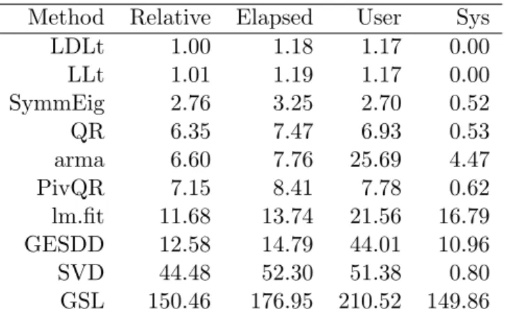
Results obtained on a desktop computer, circa 2010, are shown in Table 2. The processor used for these timings is a 4-core processor but almost all the methods are single-threaded and not affected by the number of cores. Only thearma,lm.fit,GESDDand GSLmethods benefit from the multi-threaded BLAS implementation provided by OpenBLAS, and the relative speed increase is modest for this problem size and number of cores (at 7.76 seconds relative to 10.29 seconds for arma, 13.74 seconds relative to 16.91 seconds for lm.fit, and 176.95 seconds relative to 193.29 seconds for the GSL). Parallel computing approaches will always have to trade-off increased communication and overhead costs against the potential gains from running multiple execution threads.
These results indicate that methods based on forming and decomposing X>X (LDLt, LLt and SymmEig) are considerably faster than the others. The SymmEig method, using a rank-revealing decomposition, would be preferred, although the LDLt method could probably be
Method Relative Elapsed User Sys LDLt 1.00 1.18 1.17 0.00 LLt 1.01 1.19 1.17 0.00 SymmEig 2.76 3.25 2.70 0.52 QR 6.35 7.47 6.93 0.53 arma 6.60 7.76 25.69 4.47 PivQR 7.15 8.41 7.78 0.62 lm.fit 11.68 13.74 21.56 16.79 GESDD 12.58 14.79 44.01 10.96 SVD 44.48 52.30 51.38 0.80 GSL 150.46 176.95 210.52 149.86
Table 2: lmBenchmarkresults on a desktop computer for the default size, 100,000×40, full-rank model matrix running 20 repetitions for each method. Times (Elapsed, User, and Sys) are in seconds. The BLAS in use is a locally-rebuilt version of the OpenBLAS library included with Ubuntu 11.10.
modified to be rank-revealing. However, the dimensions of the problem will influence the comparative results. Because there are 100,000 rows in X, methods that decompose the whole X matrix (all the methods except those named above) will be at a disadvantage. The pivoted QR method is 1.6 times faster than R’slm.fit on this test and provides nearly the same information as lm.fit. Methods based on the singular value decomposition (SVD and GSL) are much slower but, as mentioned above, this is caused in part byX having many more rows than columns. The GSL method from the GNU Scientific Library uses an older algorithm for the SVD and is clearly out of contention.
TheGESDDmethod provides an interesting hybrid: It uses theEigenclasses, but then deploys the LAPACK routine dgesdd for the actual SVD calculation. The resulting time is much faster than using the SVD implementation of Eigen which is not a particularly fast SVD method.
5. Delayed evaluation
A form of delayed evaluation is used in Eigen. That is, many operators and methods do not evaluate the result but instead return an “expression object” that is evaluated when needed. As an example, even though one writes theX>X evaluation as.rankUpdate(X.adjoint())
theX.adjoint() part is not evaluated immediately. TherankUpdatemethod detects that it has been passed a matrix that is to be used in its transposed form and evaluates the update by taking inner products of columns ofX instead of rows of X>.
As Eigenhas developed some of these unevaluated expressions have been modified. In Eigen 3.1, which is incorporated in version 0.3.1 of RcppEigen, the .adjoint() method applied to a real dense matrix copies the contents of the original matrix, flags it as row-major and interchanges the number of rows and columns. This is indeed the adjoint of the original matrix but, at one time, thewrap method for the Eigen dense matrix classes would fail on row-major matrices.
const MapMati A(as<MapMati>(AA));
return wrap(A.transpose());
Figure 13: badtransCpp: Transpose producing a run-time error in early versions of
RcppEigen.
to aMatrixXiobject before applying wrap to it. The assignment forces the evaluation as a column-major matrix. In early versions of theRcppEigen package if this step is skipped, as in Figure13, the result would have been incorrect.
R> Ai <- matrix(1:6, ncol = 2L)
R> ftrans2 <- cxxfunction(signature(AA = "matrix"), badtransCpp, + "RcppEigen", incl)
R> (At <- ftrans2(Ai))
[,1] [,2] [,3] [1,] 1 2 3 [2,] 4 5 6
Although the problem no longer persists for this particular example, the recommended prac-tice is to first assign objects before wrapping them for return toR.
6. Sparse matrices
Eigen provides sparse matrix classes. An R object of class dgCMatrix (from the Matrix
package by Bates and Maechler(2012)) can be mapped as in Figure 14.
R> sparse1 <- cxxfunction(signature(AA = "dgCMatrix", yy = "numeric"), + sparseProdCpp, "RcppEigen", incl)
R> data("KNex", package = "Matrix") R> rr <- sparse1(KNex$mm, KNex$y)
R> stopifnot(all.equal(rr$At, t(KNex$mm)),
+ all.equal(rr$Aty, as.vector(crossprod(KNex$mm, KNex$y))))
using Eigen::MappedSparseMatrix;
using Eigen::SparseMatrix;
const MappedSparseMatrix<double> A(as<MappedSparseMatrix<double> >(AA));
const MapVecd y(as<MapVecd>(yy));
const SparseMatrix<double> At(A.adjoint());
return List::create(Named("At") = At, Named("Aty") = At * y);
typedef Eigen::MappedSparseMatrix<double> MSpMat;
typedef Eigen::SparseMatrix<double> SpMat;
typedef Eigen::SimplicialLDLT<SpMat> SpChol;
const SpMat At(as<MSpMat>(AA).adjoint());
const VectorXd Aty(At * as<MapVecd>(yy));
const SpChol Ch(At * At.adjoint());
if (Ch.info() != Eigen::Success) return R_NilValue;
return List::create(Named("betahat") = Ch.solve(Aty),
Named("perm") = Ch.permutationP().indices());
Figure 15: sparseLSCpp: Solving a sparse least squares problem.
Sparse Cholesky decompositions are provided by the SimplicialLLT and SimplicialLDLT
classes in the RcppEigen package for R. These are subclasses of the SimplicialCholesky
templated. A sample usage is shown in Figure15.
R> sparse2 <- cxxfunction(signature(AA = "dgCMatrix", yy = "numeric"), + sparseLSCpp, "RcppEigen", incl)
R> str(rr <- sparse2(KNex$mm, KNex$y))
List of 2
$ betahat: num [1:712] 823 340 473 349 188 ...
$ perm : int [1:712] 572 410 414 580 420 425 417 426 431 445 ...
R> res <- as.vector(solve(Ch <- Cholesky(crossprod(KNex$mm)), + crossprod(KNex$mm, KNex$y)))
R> stopifnot(all.equal(rr$betahat, res)) R> all(rr$perm == Ch@perm)
[1] FALSE
The fill-reducing permutations are different.
7. Summary
This paper introduced theRcppEigen package which provides high-level linear algebra com-putations as an extension to theRsystem. RcppEigen is based on the modern C++library
Eigen which combines extended functionality with excellent performance, and utilizesRcpp
to interfaceRwithC++. Several illustrations covered common matrix operations and several approaches to solving a least squares problem—including an extended discussion of rank-revealing approaches. Sparse matrix computations were also discussed, and a short example provided an empirical demonstration of the excellent run-time performance of theRcppEigen
References
Abrahams D, Gurtovoy A (2004). C++ Template Metaprogramming: Concepts, Tools and
Techniques from Boost and Beyond. Addison-Wesley, Boston.
Bates D, Maechler M (2012). Matrix: Sparse and Dense Matrix Classes and Methods. R package version 1.0-10, URLhttp://CRAN.R-project.org/package=Matrix.
Eddelbuettel D (2013). Seamless Rand C++ Integration with Rcpp. Springer-Verlag, New York.
Eddelbuettel D, Fran¸cois R (2011). “Rcpp: Seamless R and C++ Integration.” Journal of
Statistical Software,40(8), 1–18. URLhttp://www.jstatsoft.org/v40/i08/.
Eddelbuettel D, Fran¸cois R (2012). Rcpp: Seamless R and C++ Integration. R package version 0.10.2, URLhttp://CRAN.R-project.org/package=Rcpp.
Fran¸cois R, Eddelbuettel D (2012). RcppGSL: RcppIntegration for GNU GSL Vectors and
Matrices. Rpackage version 0.2.0, URLhttp://CRAN.R-project.org/package=RcppGSL.
Fran¸cois R, Eddelbuettel D, Bates D (2012). RcppArmadillo: Rcpp Integration for
Armadillo Templated Linear Algebra Library. R package version 0.3.6.1, URL http: //CRAN.R-project.org/package=RcppArmadillo.
Guennebaud G, Jacob B, others (2012). “Eigen3.” URLhttp://eigen.tuxfamily.org/.
ISO/IEC (2011). “C++2011 Standard Document 14882:2011.” ISO/IEC Standard Group for Information Technology – Programming Languages – C++. URL http://www.iso.org/ iso/iso_catalogue/catalogue_tc/catalogue_detail.htm?csnumber=50372.
Kusnierczyk W (2012). rbenchmark: Benchmarking Routine for R. Rpackage version 1.0.0, URLhttp://CRAN.R-project.org/package=rbenchmark.
Meyers S (1995).More EffectiveC++: 35 New Ways to Improve Your Programs and Designs. Addison-Wesley, Boston.
Meyers S (2005). Effective C++: 55 Specific Ways to Improve Your Programs and Designs. 3rd edition. Addison-Wesley, Boston.
R Core Team (2012a). R: A Language and Environment for Statistical Computing. R Foundation for Statistical Computing, Vienna, Austria. ISBN 3-900051-07-0, URL http: //www.R-project.org/.
RCore Team (2012b).WritingRExtensions.RFoundation for Statistical Computing, Vienna, Austria. ISBN 3-900051-11-9, URL http://CRAN.R-project.org/doc/manuals/R-exts. html.
Sklyar O, Murdoch D, Smith M, Eddelbuettel D, Fran¸cois R (2012). inline: InlineC,C++,
Fortran Function Calls from R. Rpackage version 0.3.10, URL http://CRAN.R-project. org/package=inline.
Veldhuizen TL (1998). “Arrays inBlitz++.” InISCOPE ’98: Proceedings of the Second
Inter-national Symposium on Computing in Object-Oriented Parallel Environments, pp. 223–230.
Springer-Verlag, London. ISBN 3-540-65387-2.
Affiliation:
Douglas Bates
Department of Statistics
University of Wisconsin-Madison Madison, WI, United States of America E-mail: [email protected]
URL: http://www.stat.wisc.edu/~bates/
Dirk Eddelbuettel Debian Project
River Forest, IL, United States of America E-mail: [email protected]
URL: http://dirk.eddelbuettel.com
Journal of Statistical Software
http://www.jstatsoft.org/published by the American Statistical Association http://www.amstat.org/
Volume 52, Issue 5 Submitted: 2011-11-14