HAL Id: cea-02339856
https://hal-cea.archives-ouvertes.fr/cea-02339856
Submitted on 5 Nov 2019
HAL
is a multi-disciplinary open access
archive for the deposit and dissemination of
sci-entific research documents, whether they are
pub-lished or not. The documents may come from
teaching and research institutions in France or
abroad, or from public or private research centers.
L’archive ouverte pluridisciplinaire
HAL
, est
destinée au dépôt et à la diffusion de documents
scientifiques de niveau recherche, publiés ou non,
émanant des établissements d’enseignement et de
recherche français ou étrangers, des laboratoires
publics ou privés.
Target and Conditional Sensitivity Analysis with
Emphasis on Dependence Measures
H. Raguet, A. Marrel
To cite this version:
H. Raguet, A. Marrel. Target and Conditional Sensitivity Analysis with Emphasis on Dependence
Measures. 2018. �cea-02339856�
CONDITIONAL SENSITIVITY ANALYSIS 2
HUGO RAGUET∗ AND AMANDINE MARREL∗ 3
Abstract.In the context of sensitivity analysis of complex phenomena in presence of uncertainty, 4
we motivate and precise the idea of orienting the analysis towards a critical domain of the studied 5
phenomenon. For this, target and conditional sensitivity analyses are defined. We make a brief 6
history of related approaches in the literature, and propose a more general and systematic approach. 7
Nonparametric measures of dependence being well-suited to this approach, we also make a review of 8
available methods and of their use for sensitivity analysis, and clarify some of their properties. Then, 9
we focus our attention on sensitivity indices based on correlation ratio, namely Sobol’ indices, and 10
on two dependence measures: the kernel quadratic dependence measure also called Hilbert–Schmidt 11
independence criterion and the Csiszár divergence dependence measure. We propose adapted versions 12
of these tools for target and conditional analysis, by considering transformation of the output using 13
hard or smooth weight functions. Finally, we show on synthetic numerical experiments both the 14
interest of target and conditional sensitivity analysis, and the efficiency of the dependence measures. 15
We also illustrate the relevance of the proposed smooth versions for conditional estimators. 16
Key words.Sensitivity analysis, computer experiments, target and conditional sensitivity analysis, 17
dependence measure, correlation ratio 18
AMS subject classifications.62G05, 62G99 19
1. Introduction. Nowadays, many phenomena are modeled by mathematical 20
equations which are implemented and solved using complex computer programs. These 21
numerical simulators are used to model and predict the underlying physical phenomena 22
and their results can guide decisions, which can involve important financial, societal 23
and safety stakes. However, they often take as inputs a high number of numerical, 24
physical or even conception parameters. Because of a lack of phenomenon knowledge 25
and characterization or a need to investigate various configurations, many of these input 26
parameters are uncertain (or considered as such) and it is important to assess how these 27
uncertainties can affect the model output. In a probabilistic framework, the uncertain 28
parameters, also called factors, are modeled by random variables characterized by 29
probabilistic distributions. Sensitivity analysis methods are performed to evaluate how 30
input uncertainties contribute, qualitatively or quantitatively, to the variation of the 31
output. The variety of approaches and applications of sensitivity analysis brings forth 32
a diversity of objects and terms. Before presenting the goals of this document and the 33
extent of our work, we introduce a few notations. 34
In the classical framework, we assume the modeling of a phenomenonY depending 35
on a set offactors (Xi)1≤i≤d following a deterministic relation Y
def
= f(X1, . . . , Xd),
36
f being the numerical simulator in our industrial applications and Y the output(s) 37
of interest. Uncertainties are taken into account by modeling the factors as random 38
variables, defined over the same implicit probability space (Ω,F,P) withΩdenoting 39
the sample space,Fthe set of events and P the associated probability measure. It will 40
also be convenient to consider a generic random variable X, usually standing for a 41
group of one or several factors. For such a variable, we note its rangeX def
= ran(X) and 42
its law PX
def
= P◦X−1is the induced probability measure overX. We also particularize
43
the range of the outputY def= ran(Y). 44
∗CEA, DEN, DER, SESI, LEMS, F-13108, Saint-Paul-lez-Durance, France;[email protected], [email protected]
1.1. Global, target and conditional sensitivity analysis. Global sensitivity
45
analysisaims at measuring how the variations of one or several factors contribute to 46
the variation of the studied phenomenon, over the whole domain of possible values. 47
Many authors agree with Saltelli et al. (2008) to distinguish several use of sensi-48
tivity analysis. First, the ranking of factors by importance is the starting point of 49
any application. Identifying the factors which are most influential in a phenomenon 50
might help understanding it or guide resource investment for controlling it. Then, 51
screeningthe factors for insignificant ones is considered, for instance for the purpose of 52
model simplification. This sometimes calls on statistical tests, which might be practical 53
but cannot be satisfying for all applications. In our experience, screening is often in 54
practice interpretation of ranking, either through the expertise of the practitioner or 55
with some cross-validation process. Finally, factor mapping is often described as a 56
finer identification of functional relationship between the specific domains of values 57
of the factors and of the phenomenon. This last use of sensitivity analysis consists 58
in determiningwhich values of these factors are responsible of the occurrence of the 59
phenomenon in a given domain. 60
61
In our work, we also focus on specific domains of values of the phenomenon 62
but we want to determine which factors contribute most in the occurrence of the 63
phenomenon in a given domain. For this, we first define thetarget sensitivity analysis
64
which aims at measuring the influence of the factors over a restricted domain of the 65
studied phenomenon, and in particular over theoccurrence of the phenomenon in this 66
restricted domain. Such domain of interest would usually be extreme and relatively 67
rare, constituting a risk or an opportunity; we call itcritical domain, notedC ⊂ Y and 68
associated to acritical probability P(Y ∈ C) = PY(C). Alternatively, we also define the
69
conditional sensitivity analysiswhich evaluates the influence of the factorswithin the 70
critical domain only, ignoring what happens outside. Let us underline that those two 71
notions can widely differ; this point will be illustrated by the numerical applications 72
proposed in this paper. 73
1.2. Goals and Structure of the Paper. In this paper, we aims at proposing 74
news methods and tools for target and conditional sensitivity analysis. It seems to 75
us that there are numerous, direct applications, especially for, but not restricted to, 76
industrial safety. Still, while global sensitivity analysis has been an active research field 77
for several decades, it seems that target sensitivity analysis is less understood, and 78
until recently has not been studied systematically as such. This is why we sometimes 79
introduce our own terminology, which we discuss along with the description of similar 80
concepts that we identify in the literature. Finally, let us point out that we are mostly 81
interested in phenomena influenced by many factors and of which only limited under-82
standing is available. Typical situations include complex systems observed through 83
heavy computer simulations or costly physical measures. These applicative constraints 84
should be taken into account when selecting and proposing dedicated tools. 85
86
Insection 2, we propose a review on the existing approaches and tools for target 87
sensitivity analysis before introducing our contributions in this framework. Then, the 88
actual sensitivity analysis tools on which our work relies are more precisely described in 89
section 3. Insection 4, we get back to our initial problematic of target and conditional 90
sensitivity analysis: we propose a simple dedicated framework and describe some 91
resulting tools. Finally, we give numerical evaluations of our methods alongsection 5, 92
on various synthetic data. 93
2. Review on Existing Approaches. We propose here a coarse classification 94
of methods relating to target sensitivity analysis, according to both chronological and 95
methodological criteria. 96
2.1. Regional Sensitivity Analysis. The very notion of target sensitivity anal-97
ysis dates back at least toSpear and Hornberger(1980), motivated by environmental 98
science applications. The proposed methodology compares the distribution of the 99
factors within the critical domain against their distribution outside. The authors 100
choose to use theKolmogorov distance, almost systematically reused ever since: 101 sup x∈ X FX|Y∈ C(x)−FX|Y∈ Y\C(x) , 102
whereFX|A is thecumulative distribution function of a real random variableX (i.e.
103
X ⊆R) conditioned by an eventA∈Fof nonzero probability (seesection 4.1.2 for 104
details). 105
They call it regional sensitivity analysis, or sometimes generalized sensitivity 106
analysis. The former name could fit our purpose, if it was not for two inconveniences. 107
First, it evokes more of a sensitivity analysis within the critical domain (what we call 108
conditional sensitivity analysis) rather than its occurrence; second, for the past three 109
decades in the literature it referred exclusively to the above methodology. It appears 110
to be the generalization of no other method, explaining why the alternative name is 111
not used anymore. Finally, one may encounter the termMonte Carlo Filtering, which 112
might be vague and restrictive. 113
Comparing distributions conditionally to the critical domain seems a good choice 114
for target sensitivity analysis. It involves only two conditionings, which facilitates 115
its estimation, for instance with Monte Carlo method. One difficulty, mentioned by 116
the authors and common to all target sensitivity methods, arises when the critical 117
probability is low. Another deficiency pointed out by the authors is the difficulty to 118
study factors in interaction. From this viewpoint, observe that a metric comparing 119
cumulative distribution functions can be extended to multidimensional settings, which 120
would allow to regroup several factors. However, the particular metric used here, namely 121
the supremum norm over the differences, is sensitive to outliers. Both aspects make it 122
particularly unsuitable for categorical factors. 123
Strangely enough, regional sensitivity is mostly used in the literature as a mean of 124
global sensitivity analysis, the partition of the domain of values of the phenomenon 125
into several regions losing its original sense and becoming more or less arbitrary. 126
2.2. Reliability Sensitivity Analysis. Another field dealing with target sensi-127
tivity analysis is motivated by applications in structural reliability, where the term 128
reliability sensitivity analysisis commonly used. In this context, critical domains are 129
failure domains, and the developed methods are influenced by two typical features: 130
failure probabilities are small in comparison to the number of available observations, 131
and the probability distributions of the factors are assumed to be known. 132
The first methods developed seek, in a suitable transformation of the factors space, 133
to determine a “most probable failure point”, and to estimate the critical probability 134
from linear or quadratic approximations of the boundary of the critical domain around 135
that point. This yields the first- andsecond-order reliability methods, reviewed by 136
Rackwitz(2001). It is possible to give to each factor an importance measure based on 137
the position of the most probable failure point. The geometrical assumption about the 138
failure domain seems however restrictive, implying in particular that the factors have 139
a monotonous effect on the phenomenon. 140
The sensitivity measures which later prevail in the field are based on derivatives of 141
the critical probability, with respect to the parameters defining the probability laws of 142
the factors or of their transformation. This framework seems once again restrictive for 143
our purpose. Nonetheless, the approaches developed in parallel for dealing with low 144
critical probabilities deserves to be incidentally noted, because they could be adapted to 145
other sensitivity measures. Let us mention the methods based onimportance sampling
146
(see for instance the adaptation of Wu, 1994), as well as the approach ofsequential
147
Monte Carlo as proposed byAu and Beck(2001), who call itsubset simulation. As 148
further developed bySong et al.(2009) andCérou et al.(2012), the latter is based on 149
Markov chain Monte Carlo with the Metropolis–Hasting algorithm. 150
Still in the reliability context, the Ph.D. dissertation ofLemaître(2014) is the first 151
systematic study of target sensitivity analysis. With this purpose in mind, the author 152
compares more general methods of global sensitivity analysis, of which we give a brief 153
overview below. We can already mention that he identifies the need to transform the 154
variable modeling the phenomenon into a binary variable encoding the occurrence in 155
the critical domain; that is 1C(Y), where 1C: y7→1 ify∈ C, 0 otherwise. This is one
156
of the approach on which we focus in this work (seesubsection 4.1). 157
A first sensitivity analysis method considered is the estimation of (square)
correla-158
tion ratio between the factors and the phenomenon (real, with finite variance), 159
(2.1) η2(X, Y)def= V(E[Y|X]) V(Y) . 160
Resulting quantities are often calledSobol’(1990,1993) indices. These are nowadays 161
standard for global sensitivity analysis, notably because they can be interpreted in 162
terms of decomposition of the variance of the studied phenomenon.Lemaîtreshows 163
how these indices applied to the binary transformation of the observed phenomenon, 164
η2(X,1
C(Y)), are relevant at least for cases that are simple and where the number of
165
available observations is high enough. 166
A second method is based on the total variation which we develop later (see 167
section 3.2.2), once again applied to the binary transformation. Unfortunately, the 168
proposed estimation methods might be inadequate and the analysis is too brief; the 169
author mentions a “positive bias” without further explanations. 170
Another set of methods is based onbinary classification trees. The author lists 171
many ways of defining classification trees, and even more ways of deducing sensitivity 172
indices. This indicates a lack of generality and robustness, actually revealed by some 173
numerical experiments. For the sake of brevity, we do not elaborate here and invite 174
the interested reader to refer to the dissertation for more details. 175
Then,Lemaîtretakes over regional sensitivity described above with some modifi-176
cations. He compares the probability laws conditionally to the critical domain against 177
the (known) marginal probability laws. In addition to Kolmogorov distance, he tries 178
other discrepancy measures between cumulative distribution functions classically used 179
in statistical tests, namely Cramér–Von Mises and Anderson–Darling, and shows that 180
this choice can influence the importance ranking of factors. More importantly, he 181
suggests that sequential Monte Carlo approaches are well adapted to methods based 182
on comparisons of factor distributions conditionally to the critical domain. 183
Finally, closer to the classical sensitivity measures for reliability mentioned above, 184
the author proposes its own measures, quantifying how modifications of the factors 185
probability laws impact on the critical probability. Although it has specific advan-186
tages, such as quantification of uncertainties due to estimation errors on the model’s 187
parameters, this framework seems somewhat artificial and restrictive. 188
Altogether, this Ph.D. dissertation is an interesting entry point to target sensitivity 189
analysis. However, more numerical experiments seem necessary in order to conclude 190
about the advantages and drawbacks of the different considered approaches, and those 191
which should be retained for further improvements and comparisons are not clearly 192
identified. 193
2.3. Sensitivity Analysis of a Specific Statistic. Another recent approach 194
for target sensitivity analysis is due toFort et al.(2013). Their formulation is more 195
precise than ours: they are interested in the sensitivity ofan estimator of a statistical
196
quantityof the studied phenomenon. For this, they introduce the term ofgoal-oriented
197
sensibility analysis.1 198
From the relations V E[Y |X]
= E E[Y |X]−E[Y]2
= V(Y)−E V[Y|X] , 199
the authors show how the correlation ratio,(2.1), is, in their sense, a measure adapted 200
to the sensitivity of theexpectation of the phenomenon: indeed, it measures a distance 201
between expectations, quantified by a difference of variances. Now for a generic real 202
random variableY, expectation and variance can be defined through an optimization 203
problem, E[Y] = arg minθ∈RE
(Y −θ)2 and V[Y] = minθ∈RE
(Y −θ)2, where 204
the functional (y, θ)7→(y−θ)2 plays the role of acontrast function. 205
The generalization of the correlation ratio to a statistic defined by another con-206
trast functionψbecomes2 min
θ∈RE(ψ(Y, θ))−E(minθ∈RE[ψ(Y, θ)|X]). In practice,
207
in order to study extreme values, they focus on the quantiles of the phenomenon, 208
considering for a level α∈]0,1[, the contrast function (y, θ)7→(y−θ)(1{y≤θ}−α).
209
However, resulting indices turn out to be difficult to estimate, as shown by the recent 210
developments ofBrowne et al.(2017) andMaume-Deschamps and Niang(2017). 211
Les us mention thatKucherenko and Song(2016) propose another adaptation of 212
the correlation ratio to analysis of sensitivity of quantiles, more direct: expectations 213
are simply replaced by quantiles3of levelα∈]0,1[, E FY−|1X(α)−FY−1(α) 2 , where 214
F−1 is the generalized inverse of a cumulative distribution function. As its estimation 215
is also difficult, the authors propose to approximate the quantiles conditionally to 216
factors values by a rough form of kernel method. 217
At last, let us add that the quantile is a peculiar notion and in our opinion, its use for 218
sensitivity analysis raises some troubles. Beyond difficulty of definition and estimation, 219
these tools are adapted only to phenomena which are unidimensional and continuous. 220
Moreover, the “sensitivity of a quantile” has a less straightforward interpretation than 221
the sensitivity of the occurrence of a phenomenon, or of the variation of a phenomenon, 222
in a critical domain. 223
2.4. Contributions. The majority of the methods previously described are 224
originally developed for particular applications; we would like to make abstraction 225
of the problem to get more general methods. To this end, rather than defining or 226
enhancing specific methods, we seek modifications or generalizations of global sensitivity 227
analysis tools, which would be adapted to target or conditional sensitivity analysis. 228
Such modifications boil down, for a given analysis tool considered, to weighting 229
the observations according to the critical domain. The weights can operate following 230
1Beware that this term already exists in the literature referring to tools of different nature. 2Provided that the random variable minθ
∈RE[ψ(Y, θ)|X] is well defined. 3The random variableF−1
two principles: either as atransformationof the phenomenon prior to the application 231
of the tool, or as amodification of the parameters and objects which define the tool 232
itself. This includes, but is not restricted to, the natural notion of conditioning. Several 233
variations around these principles are presented alongsection 4; before that, the actual 234
sensitivity analysis tools must be introduced. 235
3. Correlation Ratio and Dependence Measures for Sensitivity Analy-236
sis. We present here the measures of sensitivity analysis upon which we construct our 237
tools. First, sensitivity indices based on correlation ratio, the popularSobol’ indices, 238
are introduced. Now, it appears that sensitivity analysis based on nonparametric
239
dependence measures, recently advocated byDa Veiga (2015), is particularly adapted 240
to our framework. This will retain most our attention in the following, starting from 241
subsection 3.2where we review available methods for measuring statistical dependence 242
and detail the use of some of them in the context of sensitivity analysis. 243
3.1. Correlation Ratio yielding Sobol’ Indices. Given a group of factors 244
I ⊂ {1, . . . , d}, we write XI
def
= (Xi)i∈I for the corresponding random tuple, and
245
c
I def={1, . . . , d} \I for the complementary group of factors. Moreover, we abusively 246
note the concatenation XI, XcIdef= Xi
1≤i≤d.
247
The use of correlation ratio for sensitivity analysis has been proposed byIman
248
and Hora(1990) andIshigami and Homma(1990), and independently bySobol’ (1990, 249
1993). The latter was the most popularized, introducing modifications of correlation 250
ratios of groups of factors to achieve a convenient decomposition of the total variance 251
of the phenomenon, provided that the factors are independent; these are the Sobol’ 252
indices. While they are theoretically interesting for studying specific interactions of 253
factors, in practice the most useful sensitivity indices are thefirst-order indicesand the 254
total-order indices. The former tends to evaluate the influence of a group of factorI
255
on its own and is simplyη2(X
I, Y), and the latter incorporate all possible interactions
256
with other factors, defined as 1−η2 Xc
I, Y
. 257
Estimation of correlation ratio can be expensive because it involves the term 258
E E[Y |XI]2. Most common efficient estimators develop the square conditional
ex-259
pectation as the product Ef(XI, XcI)XI
Ef(XI, X0cI)XI
where (XI, X0cI) is 260
distributed identically to (XI, XcI), which in turn is Ef(XI, XcI)f(XI, X0cI)XI,
261
provided thatXcI andX0cI are independent conditionally toXI. In practice, this is 262
ensured when theinput factors are independent. The expectation of the last expression 263
is nothing but E f(XI, XcI)f(XI, X0cI), which is now easier to handle. Typical esti-264
mator consists in drawing 2nindependent observations XI(j), Xc(Ij)
1≤j≤2n distributed
265
as XI, XcI, and evaluating the model at specifically chosen factors combinations, 266 typically 267 (3.1) E E[Y |XI]2n def = 1 n n X j=1 f XI(j), Xc(Ij) f XI(j), Xc(In+j) . 268
Let us mention that this approach, usually referred to as pick-and-freeze, has two 269
drawbacks: first, this constrains theexperience design (the set of points at which the 270
model must be observed or computed), and second, the required number of model 271
evaluations grows with the number of factors to be investigated. 272
3.2. Sensitivity Analysis with Dependence Measures. Sensitivity analysis 273
based on correlation ratio as described above is fairly general and can be readily adapted 274
for target and conditional analysis, as we propose later in sections 4.2.1and 4.2.2. 275
However, several weaknesses can be pointed out. 276
First, accurate estimation is known for requiring many observations. In addition, 277
although statistical independence implies zero correlation ratio, some variables can 278
be significantly related and yet their correlation ratio be zero as well; in such case, 279
one must resort to total-order indices to identify a relationship. More generally, the 280
statistical variance of the phenomenon might not be the most representative mode of 281
variation. Finally, the above extension for multidimensional phenomenon might not be 282
satisfying. In the classical probabilistic framework, we believe withDa Veiga(2015) 283
that a more general and more versatile notion of sensitivity of a phenomenon to a group 284
of factors can be captured by the notion of statistical dependence. Moreover,De Lozzo
285
and Marrel(2016) recently investigated the use of dependence measures for sensitivity 286
analysis of costly model and illustrated the efficiency of associated significance tests 287
for screening purpose. 288
We propose somewhere else (Raguet and Marrel,2018, §§ 3.1 and 3.2), a classifi-289
cation of dependence measures in general, and an extensive discussion on their use for 290
sensitivity analysis in particular. We refer the interested reader to the above article for 291
details; for now, let us focus on two important classes. Note that our choice is mainly 292
guided by ease of implementation (notably the possibility of writing estimators as 293
empirical expectations), aim for generality (factors and phenomenon of any nature 294
and dimension), good invariance properties, and ease of adaptation for target and 295
conditional sensitivity analysis. They both rely on the same principle: measuring 296
the statistical dependence between two variablesX andY by comparing their joint 297
distribution PX,Y to their product PX⊗PY; the two being equal if, and only if,X
298
andY are independent. 299
3.2.1. Kernel Quadratic Dependence Measure also called Hilbert–Schmidt 300
Independence Criterion. The first class of dependence measures which we consider 301
arises in the literature from the comparison of the distributions according to their 302
probability densityorcharacteristic functions, with help of weightedL2norms. However,
303
more recent interpretations in terms ofkernel embeddings of probability distributions 304
yield thekernel quadratic dependence measure, following the terminology ofAchard
305
et al.(2003) andDiks and Panchenko(2007), also calledHilbert–Schmidt independence
306
criterionbyGretton et al.(2005). 307
In brief, if P is a probability distribution over a generic spaceZ, and ifk:Z2→
R
308
is a suitable positive definite kernel, then the mapping z 7→ R
k(z, z0) dP(z0) is an 309
element of thereproducing kernel Hilbert space induced byk (see the introduction 310
of Berlinet and Thomas-Agnan, 2003, Chapter 4). The norm between such kernel
311
embeddingsof two different probability distributions is called theirkernel distance. 312
A measure of the dependence between X and Y is thus defined by the ker-313
nel distance between PX,Y and PX⊗PY. These are probability distributions over
314
the space X × Y; a useful particular case arises when the kernelk is separable as 315
((x, y),(x0, y0))7→ kX(x, x0)kY(y, y0), where kX andkY are positive definite kernels
316
overX and Y, respectively. The square of the resulting kernel distance is the kernel 317
quadratic dependence measure, and can be expressed as 318 319 (3.2) QDMkX,kY(X, Y) def = 320 E(kX(X, X0)kY(Y, Y0)) + E(kX(X, X0)) E(kY(Y, Y0))−2 E(kX(X, X0)kY(Y, Y00)), 321 322
provided that (X0, Y0) is independent of, and distributed identically to, (X, Y), and 323
Y00 is independent ofX, Y, X0, Y0 and distributed identically toY. 324
A straightforward estimator, given X(i), Y(i) 1≤i≤n independent observations 325 distributed identically to (X, Y), is 326 QDMkX,kY(X, Y)ndef= 1 n2 n X i,j=1 kX X(i), X(j)kY Y(i), Y(j) + 1 n2 n X i,j=1 kX X(i), X(j) 1 n2 n X i,j=1 kY Y(i), Y(j) − 2 n n X i=1 1 n n X j=1 kX X(i), X(j) 1 n n X j=1 kY Y(i), Y(j) , 327
which should be put under the following handier form for practical implementation, 328 1 n2 n X i,j=1 kX X(i), X(j)− 1 n n X `=1 kX X(i), X(`) kY Y(i), Y(j)− 1 n n X `=1 kY Y(`), Y(j) . 329
Note that some authors prefer normalizing with factorsn−1 andn−2, or add some 330
other debiasing modifications, which are of little interest here. The required number 331
of computations grows asO(n2), which is acceptable in situations where the cost for
332
obtaining each observation is large. 333
WhenX is a finite set, thecategorical kernel (x, x0)7→1 ifx=x0, 0 otherwise, is 334
most typically used. WhenX is a normed vector space, theGaussian kernel (x, x0)7→
335
exp −kx−x0k2
2σ2for some parameterσ2∈R, dependent in practice on the data, 336
is also typically used, but others variants are popular;Sejdinovic et al.(2013) show 337
that thedistance covarianceofSzékely et al.(2007) is a particular case. 338
These last authors propose to normalize their dependence measure in the spirit 339
of the linear correlation coefficient, yielding thedistance correlation, which is scale-340
invariant. When Da Veiga (2015) highlights the potential use of the quadratic de-341
pendence measure for sensitivity analysis, he also advocates for such normalization, 342
leading to the sensitivity index 343 QDMkX,kY(X, Y)def= QDMkX,kY(X, Y) q QDMkX,kX(X, X)qQDMkY,kY(Y, Y) , 344
and similarly for itsplug-inestimator QDMkX,kY(X, Y)n. 345
3.2.2. Csiszár Divergence Dependence Measure. The second class of de-346
pendence measures which we consider compares the distributions through Csiszár
347
(1972) divergences. Considering again P,Q two probability distributions over a generic 348
spaceZ, aCsiszár divergencebetween P and Q can be defined as 349 divφ(P,Q) def = Z φ dP dQ dQ, 350
where φ:R+ →R∪ {+∞} is a convex function vanishing at unity, and dPdQ is the
351
Radon–Nikodym derivative of P with respect to Q; note that this can be conveniently 352
extended to cases where P is not dominated by Q. Notable examples include the 353
(reverse) Kullback–Leibler divergence with φ:t 7→ −log(t) and the total variation
354
distance withφ:t7→ |t−1|. 355
Again, one can measure dependence betweenX andY by measuring discrepancy 356
between PX,Y and PX⊗PY with help of this tool, yieldingCsiszár divergence
depen-357
dence measure, CDMφ(X, Y)
def
= divφ(PX⊗PY,PX,Y). The famous special case of the
358
mutual information, stemming from the work of Shannon(1948), is obtained with the 359
Kullback–Leibler divergence, div−log(PX⊗PY,PX,Y). In the context of sensitivity
360
analysis,Park and Ahn(1994) use a form of mutual information, and laterBorgonovo
361
(2007) uses the total variation dependence measure. In both cases, estimating the 362
Csiszár divergence is problematic, and the authors must call onad hoc parametric 363
density fits. 364
In fact, estimations of Csiszár divergences have been studied in many contexts, often 365
focused on specific versions defined by a given functionφor on specific knowledge about 366
the involved distributions. In order to devise a general tool, we choose in the current 367
work to rely on nonparametric estimations of the Radon–Nikodym derivatives. Densities 368
at specific points can be estimated throughkernel ornearest-neighborsmethods, see for 369
instance the monograph ofSilverman(1986). Probabilities are estimated by empirical 370
frequencies. Both can be combined if necessary. 371
We justify somewhere else (Raguet and Marrel, 2018, § 3.4.2) that a “support” 372
version, sCDMφ(X, Y), where the integration is performed over the range of the
373
joint variable (X, Y) rather than the whole product spaceX × Y, is convenient. The 374 corresponding estimator is 375 (3.3) sCDMφ(X, Y)kX,kY,n def = 1 n n X i=1 φ 1 n Pn j=1kX X (i), X(j)1 n Pn j=1kY Y (i), Y(j) 1 n Pn j=1kX,Y X(i), Y(i), X(j), Y(j) 376
wherekX,kY andkX,Y are the kernels used for estimating densities or probabilities;
377
typically (normalized) Gaussian and categorical, respectively. It has a computational 378
cost ofO(n2), just as for the kernel quadratic dependence measure.
379
Unfortunately, normalization is not as natural as for the kernel quadratic depen-380
dence measure which derives from a square norm. Consider moreover that, for instance, 381
sCDMφ(X, X) might be infinite. We propose to normalize the estimatorsas
382 sCDMφ(X, Y)kX,kY,n def = sCDMφ(X, Y)kX,kY,n sCDMφ(X, X)kX,kX,n . 383
Let us mention to the interested reader that this can be seen as a rough generalization 384
of the normalization proposed by Joe(1989) for mutual information of categorical 385
variables, because sCDM−log(X, X) is in that case theShannon entropy ofX.
386
4. Some Tools for Conditional and Target Sensitivity Analysis. All of 387
the sensitivity measures detailed above can be easily adapted to target and conditional 388
sensitivity analysis. We describe first general approaches which can be applied to any 389
sensitivity measure. Further details are then given for each tool that we consider. 390
4.1. Transformations and Weights. Our general approaches are based on 391
transformations of the variable quantifying the phenomenon and on conditioning; 392
specific notions and notations are introduced here. 393
4.1.1. Targeting with Transformations. In order to study theoccurrencesof 394
the phenomenonY within the critical domainC ⊂ Y, the natural transformation which 395
comes to mind is a binary random variable encoding directly the actual phenomenon of 396
interest and suppressing uninformative fluctuations. This leads to consider the weight 397
function 1C: Y → {0,1}:y7→1 if y∈ C, 0 otherwise.
398
Now, recall that a limited number of observations is usually assumed, so that 399
estimation considerations cannot be ignored. The binary transformation above might 400
result in a significant loss of the information conveyed by the relative values of Y. 401
Indeed, when the critical probability PY(C) is low, most data is summed up to a bunch
402
of zeroes. 403
Fortunately, a sensible relaxation of the binary assumption can be given as soon as 404
one can evaluate some sort of distancedC:Y →R+ between each point inY and the
405
critical domainC. One can compose it by a decreasing real functionR→[0,1], with 406
the rationals that the closer is an observation to the critical domain, the more likely it 407
is to convey similar information. This of course assumes some kind of regularity of the 408
phenomenon’s statistical properties. WhenY lies in an Euclidean space, we typically 409
consider the weight functiony7→exp(−dC(y)/s), wheredC(y)
def
= infy0∈Cky−y0k. Here,
410
the exponential function encodes multiplicative contributions, andsis a smoothing 411
parameter depending typically on a measure of dispersion of the values ofY. 412
In all the following,w: Y →[0,1] is any kind of the above weight functions, either 413
used deterministically, or as a transformation yielding a random variable through the 414
compositionw(Y). Any sensitivity measure between a group of factorsX andw(Y) 415
yields a target sensitivity measure. 416
4.1.2. Conditioning with Weighted Probabilities. Alternatively, in order 417
to study thebehavior of the phenomenon within the critical domain, a natural idea 418
is conditioning by the event {Y ∈ C}. Given an initial probability space (Ω,F,P), 419
if A ∈ F is an event of nonzero probability, then conditioning by A simply means 420
endowing the measurable space (Ω,F) with the probability measure P|A, defined as
421
P|A(B)
def
= P(B∩A)
P(A) for allB∈F. IfX is a random variable over (Ω,F,P), then 422
its law conditionally toAis the law of the mappingX over the conditioned probability 423 space Ω,F,P|A , that is PX|A def = P|A◦X−1. 424
Just as we introduced smooth relaxation of the binary transformation above, it 425
might be useful to consider extensions of conditioning allowing to take into account 426
some of the information outside the critical domain. This can be easily done by 427
observing that P|A(B) can be expressed as
R
B1AdP
R
Ω1AdP. IfW is a positive
428
nonzero random variable over (Ω,F,P) with finite expectation, we define theprobability
429
P weighted by W, noted PW, with for all B ∈ F, PW(B)def= R
BWdP
R
ΩWdP. In
430
other words, PW is the probability distribution absolutely continuous with respect to P 431
whose density is proportional toW. In addition, ifX is a generic random variable, we 432
clarify that the notation PWX stands for the image measure PWX; although strictly 433
speaking, it cannot be confused with a weighted image measure (PX) W
since W is 434
defined overΩand not over the range ofX. Let us also exemplify the particular cases 435
of weighted probabilities which are actual conditional probabilities, P|A= P1A, and
436
PX|A= P
1A
X.
437
In a probabilistic framework, any sensitivity measure is defined depending on a 438
(usually implicit) probability space. When conditioning by weight W, we change the 439
underlying probability measure, but the mappings defining the random variables are 440
left unchanged; in such case, the notations are prefixed by PW. Let us underline 441
here that, provided that the expectations exist, PW
E(X) = E(W X) E(W),. 442
For conditional sensitivity analysis, we typically use conditioning by weights 443
W set=w(Y) as defined above. 444
4.2. Correlation Ratio. As presented insubsection 3.1, sensitivity indices based 445
on correlation ratio (widely known as Sobol’ indices) all consists in (possibly weighted 446
sums of) correlation ratios of the phenomenonY with well chosen groups of factors, 447
noted genericallyX. 448
4.2.1. Target Correlation Ratio. Correlation ratios can be directly applied 449
to the transformation w(Y), yielding target sensitivity analysis indices based on 450
η2(X, w(Y)). Observe that even for multidimensional Y, the transformation w(Y)
451
takes values in [0,1], thus sparing us the trouble of interpreting multidimensional 452
extensions of correlation ratio. 453
4.2.2. Proposition of Hybrid Conditional Correlation Ratio. Following 454
section 4.1.2, the correlation ratio conditioned by the critical domain is the quantity 455
Pw(Y)
η X, Y
. It is important to note that even if the factors are independent 456
under P, they usually are not under Pw(Y). The covariance estimator in(2.1)cannot
457
be used anymore, hindering the estimation of the correlation ratio as explained in 458
subsection 3.1. 459
Alternatively, it is possible to define a conditional correlation ratio by another 460
transformation ofY. We have seen thatw(Y), keeping no memory of the actual values 461
ofY, is more adapted to target sensitivity; for conditional sensitivity, it is preferable 462
to weight multiplicatively the values, asw(Y)Y. However, the fact thatwvanishes on 463
regions away from the critical domain seems arbitrary: the value zero might not be 464
meaningful for the phenomenon at hand. Since the correlation ratio is a measure of 465
variance, it still seems relevant to set a constant value over these regions, but equal to 466
the expectation of the resulting transformation; they would then not contribute to the 467
variance of the phenomenon. We thus define the transformation 468
Yw
def
=w(Y)Y+(1−w(Y))y0 such that y0def= E(Yw) ; yielding y0=
E(w(Y)Y) E(w(Y)) . 469
Observe that with w set= 1C, E(w(Y)) = P(Y ∈ C) and y0 = E[Y |Y ∈ C]; more
470
generally, we have y0 = Pw(Y)E(Y). In any case, it is easy to estimate with 471 Pn i=1w(Y (i))Y(i) Pn i=1w(Y (i)), andη2(X, Y
w) can be estimated in turn with any
472
usual method, with the advantage over the conditional correlation ratio that even 473
observations associated to null weight are somehow taken into account. 474
4.3. Kernel Quadratic Dependence Measure. We recall that this depen-475
dence measure is also known as Hilbert–Schmidt independence criterion, and is detailed 476
insection 3.2.1. 477
4.3.1. Target Kernel Quadratic Dependence Measure. Just as with the 478
correlation ratio, target sensitivity measure of a group of factors can be obtained 479
through the weight transformationsw(Y), that is to say QDMkX,k
w(Y)(X, w(Y)). Our
480
notation reminds that the kernels depend on the underlying spaces; in the particular 481
case of the binary transformationwset= 1C, it seems natural to use a categorical kernel for
482
k{0,1}. Let us mention that this last case was already suggested and briefly illustrated
483
byDa Veiga(2015). 484
4.3.2. Conditional Kernel Quadratic Dependence Measure. The condi-485
tional versionPw(Y)
QDMkX,kY(X, Y) is defined through kernel distance and can 486
be again expressed as expectations of kernels analogously to(3.2) 487 E(kX(X, X0)kY(Y, Y0) ¯w(Y) ¯w(Y0)) + E(kX(X, X0) ¯w(Y) ¯w(Y0)) E(kY(Y, Y0) ¯w(Y) ¯w(Y0)) −2 E(kX(X, X0)kY(Y, Y00) ¯w(Y) ¯w(Y0) ¯w(Y00)), 488
having taken care of normalizing the weights ¯w def= E(w(Y))−1w. This can also be 489
analogously estimated, by replacing empirical averages by weighted averages 490 n X i,j=1 kX X(i), X(j)− n X `=1 kX X(i), X(`)w Yˆ (`) ! × kY Y(i), Y(j)− n X `=1 kY Y(`), Y(j)w Yˆ (`) ! ×w Yˆ (i) ˆ w Y(j) , 491
with empirical normalized weights ˆwdef= Pn
i=1w Y (i)−1
w. 492
4.4. Csiszár Divergence Dependence Measure. We refer to section 3.2.2
493
for the definitions of the “support” Csiszár divergence dependence measure. 494
4.4.1. Target Csiszár Divergence Dependence Measure. As previously, 495
target sensitivity measure of a group of factors can be obtained through Csiszár diver-496
gence dependence measures of the transformationsw(Y), that is to say sCDMφ(X, w(Y)).
497
Let us emphasize that, in the case of the binary transformation w set= 1C, Radon–
498
Nikodym derivatives should be estimated with normalized categorical kernel. 499
4.4.2. Conditional Csiszár Divergence Dependence Measure. The condi-500
tional versions are respectively Pw(Y) CDMφ(X, Y) = divφ PX,Yw(Y),PXw(Y)⊗PwY(Y) 501 andPw(Y) sCDMφ(X, Y) = sdivφ
PwX(Y)⊗PYw(Y),PwX,Y(Y). In the estimator in(3.3), 502
the weights are influencing the expectations in each density estimation and each integral, 503
yielding with empirical normalized weights ˆwdef= Pn
i=1w Y (i)−1 w, 504 n X i=1 φ Pn j=1kX X (i), X(j) ˆ w Y(j)Pn j=1kY Y (i), Y(j) ˆ w Y(j) Pn j=1kX,Y X(i), Y(i), X(j), Y(j)w Yˆ (j) w Yˆ (i) . 505
Versions with nearest-neighbors density estimation can also be easily adapted. For 506
instance, thek-th nearest-neighbor distance of the point (x, y)∈ X × Y is the smallest 507
distance dk such that the cumulative sum of the weights of the points within dk
508
distance to (x, y) reaches k. If copula transforms are used, recall that they are also 509
modified by weighted probabilities. 510
5. Numerical Illustrations. We conduct here numerical illustrations and com-511
parisons of the different adapted tools that we propose for target and conditional 512
sensitivity analysis. These concise examples also demonstrate that target and condi-513
tional sensitivity analysis explore aspects of a model which are both different from 514
global sensitivity analysis and valuable for practitioners. 515
Note that all the above tools are implemented in the language R, interfaced with 516
C++ for some routines; we intend to integrate them to theSensitivity package of R. 517
5.1. Presentation of Test Case Functions. To illustrate target and condi-518
tional sensitivity analysis, we first propose a model with a simple but strong nonlin-519
earity, which we callminimum-normal-uniform. It is defined in dimensiondset= 2, with 520
f:x7→min(x1, x2), with independent factors conveniently notedX1set=NandX2set=U, 521
following respectively a standard normal distribution, and a uniform distribution over 522
[0,1]. 523 524
We then explore the more complicated Ishigami–Homma model which is well-525
known from the sensitivity analysis community. This model is defined in dimension 526
dset= 3 by 527
f:x7→sin(x1) +asin2(x2) +bx34sin(x1),
528
wherea, b∈R+; all factors (X1, X2, X3) are independent and uniformly distributed
529
over [−π,π]. The influence of the factorX2 is purely additive, its importance being 530
modulated by the parametera. The influence of the factorX1 includes an additive 531
part and an interaction with the factorX3, the balance being tuned by parameter 532
b. We set here the parameters aset= 5 andb set= 0.1, so that first-order Sobol’ indices 533
areη2(X1, Y) = 0.40,η2(X2, Y) = 0.29 andη2(X3, Y) = 0, while total-order ones are 534
1−η2(Xc
{1}, Y) = 0.71, 1−η2(Xc{2}, Y) = 0.29, and 1−η2(Xc{3}, Y) = 0.31. 535
536
In both models, we suppose that the critical domainC is defined byY exceeding 537
a given critical value:Cset
={y∈ Y |y≥c}, chosen as theninth decile ofY computed 538
empirically,cset=FY,n−1(0.9). Recall that target and conditional sensitivity measures are 539
defined via weight functionsw:Y →[0,1] which depends onC. In both models, we 540
use the indicator function 1C, and a smooth relaxation in accordance with the notion
541
of distance over the reals, 542 (5.1) wC:y7→exp −max(c−y,0) s σY ; 543
where σY is an estimation of the standard deviation ofY, and s
set
= 1/5 is a factor 544
tuning the smoothness, chosen so thatwC almost vanishes one standard deviation
545
away fromC. 546
5.2. Tested Target and Conditional Sensitivity Tools. Among the large 547
choice of interesting sensitivity measures, we consider those inTable 5.1. Correlation 548
ratios estimated with pick-and-freeze factors combinations are included because they 549
are currently the most popular for global sensitivity analysis. Recall however from 550
section 4.2.2that they do not allow for proper conditional versions, because conditioning 551
introduces dependence between factors. Consequently, we use what we call the “hybrid” 552
version. We report here results only for the first-order indices, but we can mention that 553
the total-order indices behave similarly for target and conditional sensitivity analysis 554
of both analytical models. 555
Then, we include the quadratic dependence measure with Gaussian kernel, and 556
the mutual information dependence measure with truncated nearest-neighbors copula 557
density estimationBlumentritt and Schmid(2012). For the hard target versions, recall 558
that 1C(Y) is a discrete random variable over {0,1}. For the mutual information,
559
its law is estimated by empirical frequencies and the law of the joint (Xi,1C(Y)) is
560
estimated by conditioning. For the quadratic dependence measure, we use a categorical 561
kernel fork{0,1}.
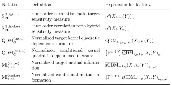
Table 5.1: Sensitivity measures used for target and conditional analysis experiments. The generic weight function wis either 1C, or the smooth relaxationwC defined in
(5.1).
Notation Definition Expression for factori
S(1,tgt,PF w) First-order correlation ratio target sensitivity measure η
2(X
i, w(Y))n
S(1,hbd,PF w) First-order correlation ratio hybrid sensitivity measure η
2(X
i, Yw)n
QDM(tgt,G w) Normalized target kernel quadratic
dependence measure QDMkX,kw(Y)(Xi, w(Y))n
QDM(cnd,G w) Normalized conditional kernel quadratic dependence measure
Pw(Y)QDMkX,kY(Xi, Y)n
MI(tgt,c,nnw) Normalized target mutual
informa-tion sCDM−log(Xi, w(Y))knn,n
MI(cnd,c,nnw)
Normalized conditional mutual in-formation
Pw(Y)sCDM−log(Xi, Y)knn,n
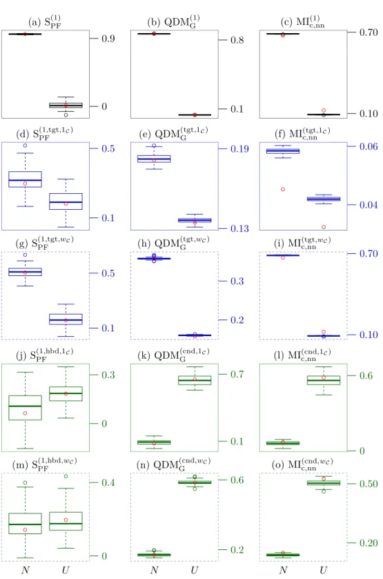
5.3. Numerical Experiments and Results. For each model, we draw hun-563
dred different samples of sizenset= 1 000 and schematize the resulting distribution of 564
each conditional or target sensitivity measure, together with their global sensitivity 565
counterpart, with Tuckey box plots onFigures 5.1and5.2. 566
On the minimum-normal-uniform model, the critical value isc= 0.62. The global 567
analysis, onFigures 5.1(a)to5.1(c), is unanimous: the factorN is much more important 568
than the factorU. This is not surprising, sinceN presents more variability and takes 569
values far below the minimum ofU. 570
The target analysis indicates that the ordering of the factors is the same, although 571
the relative importance difference is less drastic. This is again not surprising becauseN
572
has a higher probability to be below the critical value thanU, hence still determining 573
again the outcome of interest here, but in the same time, the variability ofN below the 574
threshold has no influence anymore. The correlation ratio onFigure 5.1(d), is much 575
less precise than the dependence measures(e)and(g). The target mutual information 576
shows an important bias, but this does not impact the ordering of the factors. It 577
can be noted that the smoothed versions present less variability while still ordering 578
correctly the factors. However, it is unclear if this is thanks to better behavior of the 579
smooth estimator, or simply because the estimated smoothed quantity is some kind of 580
interpolation between target and global measures. In the latter case, this effect would 581
turn out unfavorable if the ordering of the factors were different in both analysis. The 582
smoothed target mutual information onFigure 5.1(i)is clearly problematic, as it yields 583
the same importance measures as the global version(c). This can be explained by the 584
fact that the density estimation is based on copula transforms, and thatY andwC(Y)
585
have very similar copula transforms with the level of smoothing that we used; in this 586
case and for this particular estimator, smoothing is not judicious. 587
The conditional analysis tells a whole different story: nowU is more important 588
thanN. Indeed, conditionally to bothU andN being no less thanc,U varies in [c,1] 589
while N varies in [c,+∞[, in such a way that the former has more chance to determine 590
(a) S(1)PF ● ● ● 0 0.9 (b) QDM(1)G ● ● ● ● ● ● 0.1 0.8 (c) MI(1)c,nn ● ● ● ● 0.10 0.70 (d) S(1,tgt,1C) PF ● ● ● 0.1 0.5 (e) QDM(tgt,1C) G ● ● ● 0.13 0.19 (f) MI(tgt,1C) c,nn ● ● 0.04 0.06 (g) S(1,tgt,PF wC) ● ● ● 0.1 0.5 (h) QDM(tgt,G wC) ● ● ● ● ● ● ● ● 0.2 0.3 (i) MI(tgt,wC) c,nn ● ● ● ● ● 0.10 0.70 (j) S(1,hbd,1C) PF ● ● 0 0.3 (k) QDM(cnd,1C) G ● ● 0.1 0.7 (l) MI(cnd,1C) c,nn ● ● 0 0.6 (m) S(1,hbd,PF wC) ● ● ● ● 0 0.4 (n) QDM(cnd,G wC) ● ● ● ● ● ● ● 0.2 0.6 (o) MI(cnd,c,nnwC) ● ● ● 0.20 0.50 N U N U N U
Figure 5.1: Global (black), target (blue) and conditional (green) sensitivity analysis of minimum-normal-uniform model on samples of size n set= 1 000. Red circles are asymptotic values estimated on samples of sizenset= 10 000.
the value of their minimum. This is clearly captured by both dependence measures 591
considered, onFigures 5.1(k)and(l), and moreover their smoothed conditional versions 592
improve perceptibly their precision, as indicated by the relative height of the box plots 593
inFigures 5.1(n)and(o), Hybrid correlation ratio adapted to pick-and-freeze estimator 594
follows the same trend onFigures 5.1(j)and(m), but precision is not satisfying at all. 595
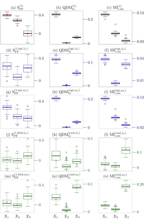
For the Ishigami–Homma model, the critical value isc= 6.31. Here, the relative 596
importances of the factors are different in each analysis case. In the global analysis, the 597
factorX1is the most important, and the factorsX2and X3 have lower importance, 598
being ranked differently according to different sensibility measures (Figures 5.2(a),(b)
599
and(f)). 600
In the target analysis,X3 has now similar importance toX1, whileX2has much
601
less. Indeed, the combined effect ofX1andX3easily exceeds the critical value, while the
602
isolated action ofX2can merely approach the critical value (recall that the parameter
603
aset= 5 is significantly less thanc). As previously, the dependence measures offer more 604
precision than the correlation ratio with pick-and-freeze estimator. It can be noted that 605
they do not agree exactly on the relative importance ofX1 andX3 onFigures 5.2(e)
606
and(f), and that the target kernel quadratic dependence measure does not differ much 607
from its global version in(b). Once again, the smoothed versions for target analysis 608
are not particularly relevant: even if they seem to slightly reduce the variability of the 609
estimators of kernel quadratic dependence measures, they completely fail to improve 610
the estimators of the mutual information computed through copula density. 611
In the conditional analysis,X3 becomes the dominant factor: being raised to the 612
fourth power, the corresponding term presents steep derivatives in the regime of high 613
values. The mutual information on Figure 5.2(l) seems the most suitable method 614
for putting this into evidence. Once again for conditional analysis, the smoothing 615
techniques do improve the quality of both dependence measures considered, even 616
enabling kernel quadratic dependence measure to capture the dominance ofX3.
617
6. Conclusion. In the context of sensitivity analysis of complex phenomena 618
in presence of uncertainty, this work motivates and precises the idea of orienting 619
the analysis towards a critical domain of the studied phenomenon. This gives rise 620
to the notions of target and conditional sensitivity analysis. We show that many 621
concepts in the literature relate to them, although usually in more specific frameworks 622
depending on considered applications. Building up on modern statistical tools, we define 623
mathematically a broad range of sensitivity measures which make as few assumptions 624
as possible on the model at hand, while remaining flexible enough to be adapted to 625
many particular situations. 626
To provide dedicated tools for target and conditional sensitivity analysis, we focus 627
our attention on the popular sensitivity indices based on correlation ratio, namely 628
Sobol’ indices, and on dependence measures which seem to us particularly well-adapted 629
to our problematic. More particularly, we consider two dependence measures: the kernel 630
quadratic dependence measure also called Hilbert–Schmidt independence criterion and 631
the Csiszár divergence dependence measure, the mutual information being a particular 632
case of the latter. For these different selected sensitivity measures, we propose adapted 633
versions for target and conditional analysis, by considering transformation of the 634
output using hard or smooth weight functions. We also propose an hybrid version for 635
correlation ratio. 636
The proposed tools are illustrated and compared on analytical test cases. These 637
experiments on synthetic data clearly illustrate the interest of target and conditional 638
sensitivity analysis which can differ from global one. They also show that dependence 639
(a) S(1)PF ● ● ● ● 0 0.4 (b) QDM(1)G ● ● ● ● ● 0 0.2 (c) MI(1)c,nn ● ● ● ● ● 0.03 0.13 (d) S(1,tgt,1C) PF ● ● ● ● 0 0.3 (e) QDM(tgt,1C) G ● ● ● ● ● ● ● ● ● 0 0.1 (f) MI(tgt,1C) c,nn ● ● ● ● ● ● 0.01 0.04 (g) S(1,tgt,PF wC) ● ● ● ● ● ● ● ● ● 0 0.4 (h) QDM(tgt,G wC) ● ● ● ● ● ● ● ● ● 0 0.2 (i) MI(tgt,wC) c,nn ● ● ● ● ● ● 0.02 0.13 (j) S(1,hbd,1C) PF ● ● ● ● ● ● ● 0 0.4 (k) QDM(cnd,1C) G ● ● ● ● ● ● ● ● ● ● ● ● 0 0.1 (l) MI(cnd,1C) c,nn ● ● ● ● ● ● ● 0 0.1 (m) S(1,hbd,PF wC) ● ● ● ● ● ● 0 0.4 (n) QDM(cnd,G wC) ● ● ● ● ● ● ● ● ● ● 0 0.1 (o) MI(cnd,c,nnwC) ● ● ● ● ● ● 0 0.20 X1 X2 X3 X1 X2 X3 X1 X2 X3
Figure 5.2: Global (black), target (blue) and conditional (green) sensitivity analysis of Ishigami–Homma model on samples of sizenset= 1 000. Filled red dots are analytical values, hollow red circles are asymptotic values estimated on samples of sizenset= 10 000.
measures are well suited for this task and are more precise than the correlation ratio. 640
Our preliminary results favor the use of kernel quadratic dependence measures rather 641
than correlation ratio. The mutual information with truncated nearest-neighbors cop-642
ula density estimation is also relevant (low variability and good capacity to capture 643
influence), but more adjustments should be required to reduce its bias. Furthermore, 644
even if more numerical explorations are necessary before drawing further conclusions, 645
the proposed smooth versions of estimators seem clearly suited for conditional estima-646
tors, especially when the number of available observations in the critical domain is 647
low. However, their use for target sensitivity analysis remains questionable yet. 648
649
Altogether, this work is a good starting point towards sensitivity measures which 650
are more powerful and more adapted to questions raised by experimenters. There is still 651
much to do before actually establishing good practice. Naturally, we do not pretend to 652
exhaustiveness, since we cannot evaluate in this work all existing dependence measures. 653
Other popular approaches of global sensitivity analysis could be adapted to target or 654
conditional sensitivity analysis. We voluntarily set those aside for brevity, but other 655
approaches such as the regional sensitivity analysis ought to be more deeply studied; 656
e.g. by considering other measures of discrepancy between probability distributions 657
rather than Kolmogorov distance. 658
Then, it is important to test the target and conditional sensitivity measures in 659
more challenging situations, it particular where the critical probability is low, or to put 660
it otherwise, where less critical observations are available. In that respect, we believe 661
that the smoothing technique is promising, if correctly tuned. Last but not least, all 662
these sensitivity measures can only be completely assessed through confrontation to 663
real data. 664
Aknowledgemement. The authors are grateful to Sébastien Da Veiga for sug-665
gesting the use of dependence measures and for fruitful discussions about target 666
sensitivity analysis, in the framework of the MASCOT-NUM Research Group. We also 667
thank Bertrand Iooss for his helpful advice, within the project "Uncertainty and model 668
validation" of the CEA-EDF-AREVA Institute. 669