Using Microsimulation to Estimate the Impact of Transportation Improvements and Operational Policy Changes on Travel Time Reliability

(1)

Using Microsimulation to Estimate

the Impact of Transportation Improvements

and Operational Policy Changes

on Travel Time Reliability

by

Reza Golshan Khavas

A thesis

presented to the University of Waterloo in fulfillment of the

thesis requirement for the degree of Doctor of Philosophy

in

Civil Engineering

Waterloo, Ontario, Canada 2017

(2)

ii

Author’s Declaration

This thesis consists of material all of which I authored or co-authored: see Statement of Contributions included in the thesis. This is a true copy of the thesis, including any required final revisions, as accepted by my examiners.

(3)

iii

Statement of Contributions

Chapter 4 of this thesis consists of a paper that was co-authored by myself, my supervisor, Dr. Bruce Hellinga, and a PHD student, Mr. A. Zarinbal. I developed and documented the methodology. Mr. Zarinbal assisted with implementing the method within software. He also designed a website to demonstrate the output.

(4)

iv

Abstract

Traditionally, traffic engineers have designed roadway networks and operational strategies to manage congestion and minimize delays during the peak demand period for some “average” or “typical” day. However, increasingly, there is concern about not only the average traffic conditions along a route (during some period of the day), but also about the variability of the required time to traverse the route. Travel times vary as a function of the departure time according to relatively predictable changes in the traffic demands (i.e. travel times are longer during the peak commuting periods than during off peak periods). However, the time to complete the same trip at the same departure time also varies from day to day. The variability of travel time, and the associated additional costs, has introduced another performance measure in transportation engineering called travel time reliability (TTR). Travel time reliability has gained significant attention among the transportation researchers and practitioners recently. In this research, we aimed to implement traffic microsimulation models in order to model travel time reliability and finally to incorporate it into the alternative comparison. The contribution areas of this research are explained briefly in the following paragraphs.

Previous work that has examined the impact of weather on the characteristics of the speed-flow-density relationship has defined the weather conditions a priori and then attempted to determine the macroscopic traffic stream characteristics for these categories. However, for the purposes of modeling travel time reliability, it is necessary to only capture those weather conditions for which the associated macroscopic characteristics are statistically different. In this research we develop a technique to distinguish distinct weather categories through an innovative method.

Also, the process of determining macroscopic traffic stream characteristics requires the calibration of a macroscopic speed-flow-density model to field data. In employing this approach, we observed that the errors associated with the estimated parameters are impacted by the number and distribution of the observation points that used to calibrate the model. Therefore, we developed models to estimate the corresponding errors of the estimated traffic parameters and found that for most practical applications, the estimation of the jam density is most sensitive to the distribution of the calibration

(5)

v

data. As a result, we suggested some specific conditions for which the jam density value should be assumed a priori rather than calibrated on the basis of the available field data.

We additionally wanted to be able to model specific weather categories. We knew the traffic flow parameters of those weather conditions from the field data and we wanted the same traffic characteristics to be simulated in the traffic microsimulation model. Therefore, we proposed and evaluated a method to map the traffic flow characteristics to the TMM input parameters. The model developed in this research is not only applicable to simulate different weather categories, but also can be used to simulate any traffic condition -within the acceptable range of the model- when the traffic flow parameters are known.

Furthermore, we aimed to monetize travel time (un)reliability. To do this we have adopted the unreliability cost in terms of the costs of arriving early or arriving late. This approach has been widely used to quantify the costs of unreliability of public transport system; however, for road transport, this construct requires that we know the scheduled travel time which, from the user’s perspective is the

anticipated travel. We carried out a stated preference survey to estimate the anticipated travel time based on the travel time distribution. On the basis of the survey responses, we proposed two models in which travelers ignore unusually long travel times when determining their anticipated travel time.

Finally, we incorporated all of these findings to create an approach to quantify the cost of travel time (un)reliability using traffic microsimulation tools. We demonstrate this approach to evaluate two road improvement alternatives. We used the traffic simulation model VISSIM to compare these two alternatives based on the travel time cost and travel time reliability cost together.

(6)

vi

Acknowledgement

First of all, I wish to praise and thank God for all His blessings. I would not have made any progress without His providence.

I would like to express my sincere gratitude to my supervisor, Professor Bruce Hellinga, for his invaluable guidance, brilliant ideas, continuous motivation and the financial support. I learned a lot from his profound knowledge and great personality. I would also like to thank my PHD examining committee members, Dr. Matthew Roorda, Dr. Jeffrey Casello, Dr. Carl Haas, and Dr. Clarence Woudsma for their time and valuable comments.

I am grateful to my friends and colleagues Wenfu Wang, Reza Noroozi, Ehsan Bagheri, Sajad Shiravi, Soroush Salek Moghaddam, Ali Sarhadi and Babak Mehran for their kind support and great friendship. My special thanks go to Mr. Amir Zarinbal for the fruitful discussions we had together and also his invaluable assistance especially in IT-related areas of my research. I additionally appreciate the Iranian Ministry of Science, Research and Technology for partially funding this research.

I am deeply indebted to my beloved parents who were my first teachers. Their unconditional love and support always inspired me through my life.

Finally, I would like to thank my wonderful wife, Maryam and my lovely daughter Zahra, for their endless love, unconditional support, encouragement, and patience which made this research possible.

(7)

vii

Dedication

Dedicated to my family:

My dearest wife, Maryam,

and my lovely daughter, Zahra

(8)

viii

List of Figures

Figure 1-1-Sources of travel time variation ... 2

Figure 1-2- Conceptual stages from data preparation to alternative analysis ... 7

Figure 1-3-Incorporation of research findings in the alternative analysis ... 9

Figure 2-1-Illustration of Van Aerde’s macroscopic speed-density-flow model ... 12

Figure 2-2-Simulated freeway section ... 16

Figure 2-3- Fundamental diagrams of the traffic flow in the simulated network ... 18

Figure 2-4- Average calibration error as a function of calibration data group number ... 22

Figure 2-5-Model calibration error as a function of sample size ... 24

Figure 2-6- Traffic parameter estimation error as a function of sample size ... 26

Figure 2-7- Van Aerde’s model calibrated to uncongested equally distributed data ... 29

Figure 2-8- Calibration error for two calibration approaches: Freekj and Fixkj ... 30

Figure 2-9- Observed vs. estimated calibration error for testing data (Freekj model) ... 34

Figure 2-10- Observed vs. estimated calibration error for testing data (Fixkj model) ... 34

Figure 3-1- Illustration of categorization schemes. ... 41

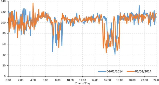
Figure 3-2-Study area ... 45

Figure 3-3- Five-minute-aggregated station speed data for two randomly selected weekdays. ... 45

Figure 3-4- Category aggregation for scheme 4 - first iteration ... 54

Figure 4-1- One trajectory for a two-parameter model ... 66

Figure 4-2-Sensitivity Analysis Procedure ... 67

Figure 4-3- Simulation Network Used for Sensitivity Analysis ... 68

Figure 4-4- Elementary Effect of Parameters ... 70

Figure 4-5- Average Normalized Elementary Effect of VISSIM Parameters ... 72

Figure 4-6- Normal Probability Plot of QEW DSD Speed Data Points ... 75

Figure 4-7- Heavy Vehicle Desired Speed Distribution ... 77

Figure 4-8- Simulation Network Coded in VISSIM ... 78

Figure 4-9- Neural Network Diagram ... 80

Figure 4-10- Validation Process ... 82

(13)

xiii

Figure 4-12- Desired vs. Simulated values of traffic flow parameters (bounded model)... 86

Figure 5-1- Illustrative 𝝉̂ and 𝝉̃ on a travel time distribution ... 93

Figure 5-2- Underlying travel time distribution ... 96

Figure 5-3- Weekday hypothetical travel times ... 98

Figure 5-4- Cumulative probability distribution of experienced travel times ... 100

Figure 5-5- Cumulative probability distribution of truncated experienced travel times ... 106

Figure 6-1- Steps within the analysis of the alternatives ... 110

Figure 6-2-Study area and the surrounding road network ... 111

Figure 6-3-Existing interchange geometry ... 111

Figure 6-4- Geometry for Alternative 1 ... 113

Figure 6-5- Geometry for Alternative 2 ... 113

Figure 6-6-Demand probability density function ... 117

Figure 6-7-Shockwave and travel time diagram of the full blockage collisions ... 121

Figure 6-8-Sampling from simulation results to generate TT distribution ... 123

Figure 6-9- Distribution of Travel Time of the route 1 ... 124

Figure 6-10- Annual cost of travel time (un)reliability ... 128

(14)

xiv

List of Tables

Table 2-1-Time Variant Demand in Simulated Network ... 17

Table 2-2-distribution of calibration data across the density bins ... 19

Table 2-3-Average calibration error as a function of the distribution of the calibration data ... 21

Table 2-4 Calibration error as a function of the distribution of the calibration data ... 23

Table 2-5-Characteristics of The Estimated Traffic Flow Parameters ... 28

Table 2-6- Comparing the Calibration Error for Freekj and Fixkj approaches ... 31

Table 2-7- Model Input Parameters ... 32

Table 2-8- Observed and Estimated Calibration Errors of both FixKj and Freekj Approaches ... 33

Table 2-9- Performance Measures for Developed Models ... 33

Table 3-1- Possible Categories ... 47

Table 3-2-Selected Calibration Approach ... 49

Table 3-3- Possible Categorization Schemes ... 50

Table 3-4- Instance of Examining the Differences between Newly Formed Categories ... 55

Table 3-5- Final categories in each categorization scheme ... 56

Table 3-6- Traffic Parameters of Final Categories in All Schemes ... 57

Table 3-7- Specifications and RMSE of the Categorization Schemes ... 58

Table 4-1-Important VISSIM Input Parameters Specified in Previous Research ... 64

Table 4-2- Rankings of VISSIM input parameters ... 69

Table 4-3- Global ranking of VISSIM input parameters ... 71

Table 4-4- Final input parameters ... 73

Table 4-5- VISSIM input parameter range ... 74

Table 4-6- Traffic demand at origins 1 and 2 ... 78

Table 4-7-Neural Network Characteristics ... 81

Table 4-8-Coefficient of Correlation of Traffic Flow Parameters ... 82

Table 4-9- Regression Model Specifications of Input and Output Traffic Flow Parameters ... 84

Table 4-10- Regression Model Specifications of Input and Output Parameters ... 84

Table 5-1-Travel Time Distribution Parameters ... 96

(15)

xv

Table 5-3- Choices in Question Regarding Extreme TT Threshold Based on DTT Percentile . 103

Table 5-4-Comparison of the Methods a and b ... 104

Table 6-1- Weather Categories with Their Traffic Flow Parameter Values ... 114

Table 6-2- Estimated VISSIM Input parameters ... 116

Table 6-3-Traffic assignment ratios ... 116

Table 6-4-Route Numbers... 116

Table 6-5-Characteristics of the Collision Scenarios... 119

Table 6-6-Values of VOT, VSDE and VSDL ... 125

Table 6-7- Illustration of TTR Cost/day Computation of Three Time Intervals - Alternative 1 126 Table 6-8- Summary of Alternative Analysis Results ... 129

(16)

1

Chapter 1 Introduction

1.1. Background

Traditionally, traffic engineers have designed roadway networks and operational strategies to manage congestion and minimize delays during the peak demand period for some “average” or “typical” day. However, increasingly, there is concern about not only the average traffic conditions along a route (during some period of the day), but also about the variability of the required time to traverse the route. Travel times vary as a function of the departure time according to relatively predictable changes in the traffic demands (i.e. travel times are longer during the peak commuting periods than during off peak periods). However, the time to complete a trip along a particular route between a specific origin and destination when the trip starts at a certain departure time (e.g. between 5 and 5:15 pm) also varies from day to day.

The variability of travel time is caused by various factors including: demand variation; insufficient road capacity; weather impacts; special events; road works; traffic management policies; and road incidents. Sources of variability have been categorized in Figure 1-1. In this figure the sources of travel time variation have been divided in two main groups: demand related and supply related sources.

(17)

2

Figure 1-1-Sources of travel time variation

The importance of arriving at the destination at a specific time is known to vary by trip type (e.g. much more important for a trip to the airport to catch a flight than a trip to the mall for shopping). Nevertheless, if the traveler has a desired arrival time, and is uncertain about the time required to travel to the destination (e.g. because of variations in travel time) then the traveler typically budgets extra time in order to be more certain of arriving on time, which increases the total travel cost considering the value of travel time (VOT) for different road users. Not only does this additional cost impact commuters, but it also impacts businesses for which punctuality is important (e.g. freight companies).

The variability of travel time, and the associated additional costs, has introduced another performance measure in transportation engineering called travel time reliability (TTR). Generally speaking, travel time is more reliable when it is less variable; meaning that the TTR is inversely proportional to travel time variability. Travel time reliability has several definitions in the literature; one of them being “the consistency or dependability in travel times, as measured from day to day and/or within different times of day” (U.S. Federal Highway Administration (FHWA), 2009).

Reliability of travel time is valuable. Casello et al.(2009) developed models that included the cost of )un(reliability as a part of the generalized cost of the transit mode while they assumed the difference between the necessary arrival time and the actual arrival time as the measure of reliability. They

•Traffic mix, drivers’ behaviour

•Seasonal effects: time, day, week, month •Demand on parallel road

•Spillback of connecting road •Traffic information

•Special events

Demand-Related

Factors

•Weather

•Road geometry and capacity •Road regulations

•Collisions

•Traffic management and control •Planned road closures

Supply-Related

Factors

(18)

3

suggested that developed models would improve the estimation of modal split in the models used for transportation forecasting.

Empirical research projects verify that the value of reliability (VOR) is larger than the value of travel time (VOT) for business trips (Warffemius, 2013). Other studies confirm that improvements made in travel time reliability are worth more than improvements of the average travel time. For instance, one study found that the cost a driver considers for mean travel time is $2.60 to $8 per hour while it is $10 to $15 per hour for standard deviation of travel time, where standard deviation is a measure of TTR (Small, 1999). The reason is that the travel time unreliability brings “scheduling cost”- the extra time the traveler budgets for the uncertainty of a route travel time - and makes the travel more expensive (Chen et al., 2003).

Travel time reliability was not the focus area in transportation engineering until the beginning of this millennium. For years, when authorities aimed to improve the performance of a road, the main objective was to increase the capacity and thereby to improve (reduce) the average travel time. Although the average travel time is still considered as the traditional road performance measure, travel time reliability has started to be used by practitioners as an additional measure of performance. There are several reasons for the increasing importance of travel time reliability. The most significant factor is that decision makers now consider a wider range of potential treatments for improving roadway performance. Road improvement options are no longer limited to capacity expansion through the addition of lanes. In fact, roadway expansion is becoming increasingly expensive and consequently impractical, particularly within developed urban centers. There are varieties of alternative improvement options. One example is the use of technologies to provide real-time information to travelers so that they are able to make optimal travel decisions (e.g. departure time, mode, route, etc.). Also, among the alternatives is the use of advanced traffic management strategies that are able to pro-actively control roadway corridors. The challenge with many of these alternative treatments is that although they may have significant benefits in terms of improving travel time reliability, they may have only a small impact on mean travel time. Consequently, when one is applying traditional cost-benefit evaluation methods, which rely on computing cost-benefits only in terms of improvements in the mean travel time, the associated benefits may be substantially underestimated for such alternatives.

(19)

4

Thus, ignoring the value of improving travel time reliability may bias the economic evaluation of some types of treatments which leads to the inefficient allocation of roadway improvement budgets. Furthermore, these types of treatments may also be undervalued when compared to other types of public sector investments.

There are a number of travel time reliability measures in the literature, all defined based on the characteristics of the travel time distribution. If the objective is to quantify the reliability of an existing corridor, then the travel time distribution can be determined by obtaining travel times from all (or a sample) of the vehicles travelling along that corridor over a period of many days. The common practice is to obtain field data for a period of at least one year.

However, if the objective is to evaluate the impact that one or more proposed roadway improvements or changes in policy (i.e. alternatives) will have on travel time reliability, then it is necessary to use models to estimate the travel time reliability for each potential future alternative.

Analytical models and traffic micro-simulation models (TMM) are two different tools that can be used to estimate the travel time reliability.

One of the earliest attempt to develop an analytical model to explain travel time variation was suggested by Herman and Lam (1974). They suggested the relationship between the mean (𝜏̅) and the standard deviation (𝜎) of travel time could be explained with the following empirical regression:

b

a

(



)

 

(1-1)

in which 𝑎 and 𝑏 are estimated regression parameters. Other researchers including Richardson and Taylor (1978) and Eliasson (2007) developed analytical models to relate the mean and the standard deviation of travel times. Some other researchers including Park et al (2010), and Tu et al (2008) studied the relationship between travel time variation and road incidents, while other researchers such as Kwon (2011) investigated the weather-related impacts on the travel time variation. Some of these models consider the TTR metrics as the dependent variable, and the factors that impact TTR as independent variables. Other analytical models estimate travel times for different situations (e.g.

(20)

5

roadway geometry, traffic demands, weather, etc.) and calculate the distribution of travel times based on the probability of those situations (Cambridge Systematics, 2013).

1.2. Problem Statement

Analytical models offer the following advantages:

 They are typically easy to apply and require relatively little field data for input.

 The relationships between the independent variables (e.g. sources of variation) and the dependent variable (e.g. TTR) are explicitly defined by the analytical model and therefore are easier to understand.

However, analytical models typically suffer from the following limitations:

 They require an extensive set of field data, including a wide range of locations, on which to calibrate the model;

 The model may not be transferable to locations that were not included in the original calibration data set;

 They cannot be used to evaluate the impacts of new designs, technologies, or policies for which no field data are available; and

 They typically only estimate a single characteristic of the travel time distribution (e.g. Standard deviation) rather than the distribution itself.

In contrast, traffic micro-simulation models could be used to estimate the impact of roadway improvements or policy changes on travel time reliability. The conceptual approach is to use the TMM to simulate a large number of “days”. TMM inputs would be varied so that each “day” would reflect different demand and supply factors which impact the travel time distribution. Essentially this is a Monte Carlo simulation approach (Bindel and Goodman, 2009) for estimating distributions given a model (in this case the TMM) and distributions for a number of model input parameters (in this case parameters to reflect the demand and supply factors that impact travel time reliability). Monte Carlo simulation consists of running the model multiple times (trials); each time randomly selecting the values from the input parameter distributions. As the number of runs increases, the estimation of the

(21)

6

distribution of the output measure of performance begins to more closely approximate the true distribution. Consequently, the use of TMM offer the following advantages:

 Field data are required only from the site being investigated;

 TMM permit the incorporation of as many factors as desired into the analysis process by designing different scenarios;

 TMM permit estimation of the entire travel time distribution (for each O-D, each route, each link, etc.); and

 TMM are already commonly being used to perform evaluations of the impacts (e.g. average travel time; emissions, etc.) of potential roadway improvements and therefore extracting measures that capture the impact on TTR might be done with very little additional effort. However, the use of traffic micro-simulation models presents the following challenges:

 Input factors (e.g. weather) required to be characterized clearly; however, it is not clear how they should be characterized. For instance, it is not clear how many distinct weather categories are really available to be simulated in TMM.

 Most TMM do not define input parameters that map directly to factors that cause travel time variability in the real world (e.g. weather). Consequently, there is a need to map variations in these factors to model input parameters.

Finally, even when the travel time distribution can be estimated (whether by TMM or some analytical model), there is a question of how this distribution can be used to make decisions about the relative preference of one alternative versus another.

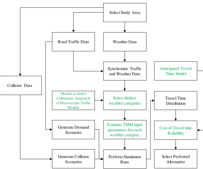
This thesis addresses these challenges. Figure 1-2 illustrates the conceptual process of performing an evaluation of alternatives using TMM. The following provides a brief introduction of each stage in this process and identifies the areas in which this thesis makes novel contributions to the state of art.

Field Data

The study area in which the travel time reliability is computed is introduced to the traffic microsimulation models through the field data. The field data required for the travel time reliability is

(22)

7

usually the archived data of at least one year or more. The data should be cleaned and prepared for the further steps.

Scenario Generation

To incorporate the impact of the travel time variability factors, TMM scenarios should be generated. In this research, we considered the demand variation as the demand-side traffic variation factor as well as weather variation and vehicle collisions as the two supply-side variability factors.

Figure 1-2- Conceptual stages from data preparation to alternative analysis

One of the significant areas of contribution of this research is the development of methods for incorporating the effects of weather within the TMM. There are three contributions in this area, namely (1) a method was developed to determine the preferred approach for calibrating a macroscopic speed-flow-density model on the basis of field data reflecting a specific weather/road surface condition; (2) a method was developed to determine statistically distinct weather/road surface condition categories; and (3) models were developed to permit the estimation of TMM input parameter values that represent a traffic stream with a set of desired characteristics (i.e. a traffic stream with characteristics reflecting a specific weather/road surface condition).

Variability Factor n Field Data Traffic Microsimulation Runs Variability Factor 2 (e.g. collisions) Variability Factor 1 (e.g. weather) Travel Time Distribution Travel Time Reliability Cost Alternative Analysis Scenario Generation

(23)

8

Traffic Microsimulation Model

Within this research, we have chosen to use the VISSIM TMM. However, the proposed methods are applicable to any TMM.

Travel Time Distribution

The travel time values obtained from simulation runs are captured to compute the travel time distribution. Within this thesis, we propose methods for compiling and aggregating these data to be computational and data storage efficient.

Travel Time Reliability Cost

One of the challenges is translating the estimated travel time distribution into a cost value to be used within cost-benefit analyses. We propose a new method to compute the travel time reliability cost which determines cost as a function of the difference between the actual travel time and the anticipated travel time. In most previous work, anticipated travel time is considered to be the mean travel time; however, one of the contributions of this research is the use of stated preference survey data to determine a model which estimates the anticipated travel time on the basis of the travel time distribution.

Alternative Analysis

We demonstrate the proposed approach through a sample application. We compared two traffic improvement alternatives based on their travel time cost and travel time reliability cost.

Figure 1-3 shows how different modules of this research are implemented to enable us to perform alternative analysis. The contributions of this research as associated with the modules shown in green.

1.3. Thesis Outline

This dissertation is organized into seven chapters as follows: 1. Introduction

2. Determining the preferred approach for calibrating a macroscopic speed-flow-density model on the basis of empirical data

(24)

9

3. Determining road surface and weather conditions which have a significant impact on traffic stream characteristics

4. Identifying parameters to model traffic during inclement weather using microsimulation 5. Incorporate drivers’ anticipated travel time in estimating travel time reliability cost 6. Demonstrating the methodology: alternative analysis

7. Conclusions and recommendations

Note that a review of the relevant literature is provided within each chapter rather than extracted into a single separate chapter.

Figure 1-3-Incorporation of research findings in the alternative analysis

Select Study Area

Collision Data

Road Traffic Data Weather Data

Generate Collision Scenarios Generate Demand

Scenarios

Synchronize Traffic and Weather Data

Select distinct weather categories Models to Select Calibration Approach of Macroscopic Traffic Models Estimate TMM input parameters for each

weather category Perform Simulation Runs Anticipated Travel Time Model Travel Time Distribution

Cost of Travel time Reliability

Select Preferred Alternative

(25)

10

Chapter 2 Calibrating a macroscopic speed-flow-density relationship using field data

2.1. Introduction

In order to incorporate different weather conditions within a microscopic traffic simulation model, it is necessary to (i) characterize the weather conditions; (ii) determine the effect that this weather condition has on driver behavior; and (iii) select appropriate values for the simulation input parameters so that the model reflects the desired behavior. This chapter addresses step (ii) from the above list.

It is (currently) impractical to make observations regarding the behavior of individual drivers under different weather conditions. However, most large urban centers have deployed systems and sensors (e.g. induction loop detectors) to collect data regarding the characteristics of the traffic stream such as average speed and flow rate. When these data are combined with meteorological weather and/or road surface condition data, it is possible to determine the traffic stream characteristics associated with specific weather conditions.

The relationship between traffic stream speed, density and flow has been under investigation since the early 20th century. In 1935, Greenshields proposed a linear relationship between speed and density for the whole range of the density in which the parameters of the model were free-flow speed and jam density (Greenshields et al., 1935). During the following years, other researchers such as Greenberg (1959), Underwood (1961), Edie (1961), etc. suggested that speed-density relationship is nonlinear (i.e. exponential, logarithmic, or both). Some researchers (including Edie) suggested piecewise models for different ranges of the traffic density.

(26)

11

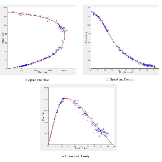
More recently, Van Aerde and Rakha (1995) suggested a four-parameter nonlinear model which provides a continuous relationship between the speed and the density. The parameters of Van Aerde’s model are free-flow speed (uf), speed-at-capacity (uc), jam density (kj), and capacity (qc). Figure 2-1 consists of two-dimensional projections of the calibrated Van Aerde’s model in terms of the relationships between: (a) speed as a function of flow; (b) speed as a function of density; and (c) flow as a function of density. The blue dots represent the observed traffic data aggregated at 5-minute intervals. The red curve is the calibrated Van Aerde’s traffic flow relationship.

(27)

12

(a)Speed and Flow (b) Speed and Density

(c) Flow and Density

Figure 2-1-Illustration of Van Aerde’s macroscopic speed-density-flow model

In this thesis, we use Van Aerde’s model to characterize the traffic stream because the model is continuous and permits all four traffic stream characteristics to be specified as parameters to the model. We point out here that from a conceptual perspective, any other continuous macroscopic traffic model could have been used. However, using a model with fewer degrees of freedom, such as Greenshields’ model, restricts the ability to reflect differences in traffic stream behavior under different weather conditions, and therefore is less desirable.

(28)

13

Thus, given a set of observed traffic data, we can calibrate Van Aerde’s model and find the associated values for the four model parameters (i.e. uf, uc, kj, and qc). Ultimately, our goal is to determine the set of weather conditions which cause statistically significant differences in these traffic stream parameters. Consequently, we want to ensure that the model parameter estimates are reliable. We hypothesize that there are two characteristics of the calibration field data set that impact the reliability of the estimated traffic stream parameters, namely: (i) the number of observations; and (ii) the distribution of the observations across density. We further hypothesize that the jam density parameter is most sensitive to these two factors and that under some conditions, it is best to fix the value of jam density rather than try to calibrate the value from the field data.

To test these hypotheses, we study the impact of the distribution of the field data over the range of the density on the error of the whole model calibration process as well as the error of each traffic parameters (i.e. free-flow speed (uf), speed-at-capacity (uc), jam density (kj), and capacity (qc)).

2.1.1. Calibrating Van Aerde’s Model

In this research, we are required to estimate the traffic flow parameters in several occasions. Here we explain how we estimate these parameters. Rakha and Arafeh (2007) showed that the functional form of the Van Aerde’s traffic flow model can be shown as:

ℎ_𝑛= 𝑐₁+ 𝑐₃𝑢_𝑛+ 𝑐2 𝑢𝑓 − 𝑢𝑛

(2-1)

where:

ℎ𝑛 : distance headway (km) between two consecutive vehicles (i.e. n-1 and n) travelling in the same lane

𝑢𝑛: speed of vehicle n (km/h) 𝑢_𝑓: free-flow speed (km/h) 𝑐₁, 𝑐₂, 𝑐₃: constants

Then as per Rakha and Arafeh (2007), Van Aerde’s model can be calibrated by solving the following optimization problem:

(29)

14 𝑀𝑖𝑛 𝐸 = ∑ {[𝑢𝑖− 𝑢̂𝑖 𝑢̃ ] 2 + [𝑞𝑖− 𝑞̂𝑖 𝑞̃ ] 2 + [𝑘𝑖− 𝑘̂𝑖 𝑘̃ ] 2 } 𝑖 (2-2) S.T. 𝑘̂_𝑖 = 1 𝑐₁+ 𝑐2 𝑢_𝑓− 𝑢̂_𝑖+ 𝑐3𝑢̂𝑖 , ∀𝑖 𝑞̂_𝑖 = 𝑘̂_𝑖× 𝑢̂_𝑖 , ∀𝑖 𝑞̂_𝑖, 𝑘̂_𝑖, 𝑢̂_𝑖 ≥ 0 , ∀𝑖 𝑢̂_𝑖 < 𝑢_𝑓 , ∀𝑖 0.5𝑢_𝑓 ≤ 𝑢_𝑐 ≤ 𝑢_𝑓 𝑞_𝑐 ≤ 𝑘𝑗𝑢𝑓𝑢𝑐 2𝑢𝑓− 𝑢𝑐 𝑐₁ = 𝑢𝑓 𝑘_𝑗𝑢_𝑐2(2𝑢𝑐− 𝑢𝑓); 𝑐2= 𝑢_𝑓 𝑘_𝑗𝑢_𝑐2(𝑢𝑓− 𝑢𝑐) 2 ; 𝑐₃= 1 𝑞_𝑐− 𝑢_𝑓 𝑘_𝑗𝑢_𝑐2 𝑢_𝑓𝑚𝑖𝑛 _{≤ 𝑢} 𝑓 ≤ 𝑢𝑓𝑚𝑎𝑥; 𝑢𝑐𝑚𝑖𝑛 ≤ 𝑢𝑐 ≤ 𝑢𝑐𝑚𝑎𝑥; 𝑘𝑗𝑚𝑖𝑛 ≤ 𝑘𝑗≤ 𝑘𝑗𝑚𝑎𝑥; 𝑞𝑐𝑚𝑖𝑛 ≤ 𝑞𝑐 ≤ 𝑞𝑐𝑚𝑎𝑥

where 𝑢𝑖, 𝑘𝑖 and 𝑞𝑖 are space-mean speed, flow, and density from the field, variables with hat (^) are estimations, and variables with tilde (~) are the maximum observations. Other variables were defined earlier. We use this formulation whenever we calibrate Van Aerde’s model in this research. Moreover, to reduce the computational cost, Rakha and Arafeh (2007) suggested to aggregate the observation points at user-defined density bins. We set the size of this density bins throughout this research at 0.25 vpkpl. We also used the built-in MultiStart algorithm in Matlab software to find the global minima of the above optimization problem in this research.

2.2. Problem Formulation

Consider that B is the set of traffic observations obtained from a traffic sensor at a location on a freeway. Observations (speed, density, flow) are aggregated and obtained over discrete time intervals (e.g. 5 minutes). B consists of observations from n time intervals such that we obtain speed (𝑢_𝑖𝑜), density

(30)

15

(𝑘_𝑖𝑜), and flow rate (𝑞_𝑖𝑜) where i = 1, n. In practice, the traffic sensors typically measure speed and flow, and then density is computed.

We calibrate Van Aerde’s traffic model using the observations in set B. The fitted curve is a line in three-dimensional space. For each observed point (𝑢_𝑖𝑜, 𝑘_𝑖𝑜, 𝑞_𝑖𝑜) we can identify the nearest point on the fitted curve (𝑢_𝑖𝑐_{, 𝑘}

𝑖𝑐, 𝑞𝑖𝑐), and the normalized Euclidean distance between these two points is designated as ‖𝑑𝑖‖ and computed as follows (H. A. Rakha and Arafeh, 2007):

‖𝑑𝑖‖ = √( 𝑢_𝑖𝑜− 𝑢_𝑖𝑐 𝑢̃ ) 2 + (𝑘𝑖 𝑜_{− 𝑘} 𝑖𝑐 𝑘̃ ) 2 + (𝑞𝑖 𝑜_{− 𝑞} 𝑖𝑐 𝑞̃ ) 2 (2-3)

In which the parameters with tilde (~) are the maximum field observation values. The model calibration error (εc

) is computed as 𝜀𝑐 =∑ ‖𝑑𝑖‖ 𝑛 𝑖=1 𝑛 (2-4)

where n is the number of observation points.

To test our hypothesis, we wish to determine the following relationship: 𝜀𝑐 _{= 𝑓(𝐵}

𝐷, 𝑛) (2-5)

In which 𝐵_𝐷 is some measure of the distribution of the traffic observations (i.e. set B) across density,

n is the number of observations and f is a function that relates the calibration error to the distribution.

2.3. Data Generation

2.3.1.

Generation

of traffic data for calibrating the macroscopic speed-flow-density

relationship

Applying the above equations to field data is challenging because: (i) the true value for the traffic stream parameters is unknown; and (ii) only a limited range of traffic conditions can be observed. Consequently, the set of traffic observations was generated from the VISSIM traffic microsimulation software. A hypothetical freeway section was coded in VISSIM (shown in Figure 2-2) and demands were varied to simulate the entire spectrum of traffic states (i.e. uncongested, capacity, and congested). The network consisted of two one-way roads: (1) and (2). The road (1) consisted of two sections. The

(31)

16

upstream section had three lanes and the downstream section had two lanes. The measurement point (i.e. location at which a traffic sensor was modelled) was located at the latter section. The road (2) had two lanes and both roads merged. The following techniques were used to create a wide range of traffic states:

1- Free flow: we defined a range of traffic demands during a number of time intervals in a way that the flow was always less than the capacity along all road sections.

2- Flow at Capacity: to experience the capacity state at the measurement point, we modelled a lane-drop upstream of the measurement point. By increasing the traffic demand entering roadway 1 to above the capacity of the two-lane section, a queue formed at the lane drop and the flow at the measurement point was equal to the capacity.

3- Traffic Congestion: we modelled a merging section downstream of the measurement point. By increasing the demand on roadway 2, it was possible to create a queue at the merging link, which would grow upstream until it spilled over the measurement point.

Figure 2-2-Simulated freeway section

The simulation time was 3.5 hours divided into 42 five-minute intervals. The simulation resolution was set to 5 time steps in each simulation second and the VISSIM default parameters were used. The first five-minute time interval was considered as warm-up period to load the network. We captured the aggregated five-minute speed, flow, and density measurements for all of the other 41 time intervals. The traffic demand values at each time interval are shown in Table 2-1.

(32)

17

Table 2-1-Time Variant Demand in Simulated Network

# Time Interval (s) Traffic Demand (vph) # Time Interval (s) Traffic Demand (vph) Road (1) Road (2) Road (1) Road (2) 1 300-600 500 0 22 6600-6900 5200 200 2 600-900 750 0 23 6900-7200 5200 400 3 900-1200 1000 0 24 7200-7500 5000 600 4 1200-1500 1250 0 25 7500-7800 1500 800 5 1500-1800 1500 0 26 7800-8100 1500 1000 6 1800-2100 1750 0 27 8100-8400 1500 1200 7 2100-2400 2000 0 28 8400-8700 1500 1400 8 2400-2700 2250 0 29 8700-9000 1500 1600 9 2700-3000 2500 0 30 9000-9300 1500 1800 10 3000-3300 2750 0 31 9300-9600 1500 2000 11 3300-3600 3000 0 32 9600-9900 1400 2200 12 3600-3900 3250 0 33 9900-10200 1300 2000 13 3900-4200 3500 0 34 10200-10500 1200 1800 14 4200-4500 3750 0 35 10500-10800 1100 1600 15 4500-4800 4000 0 36 10800-11100 1000 1400 16 4800-5100 4250 0 37 11100-11400 900 1200 17 5100-5400 4500 0 38 11400-11700 800 0 18 5400-5700 4750 0 39 11700-12000 600 0 19 5700-6000 5000 0 40 12000-12300 400 0 20 6000-6300 5200 0 41 12300-12600 200 0 21 6300-6600 5200 0

The simulation was run 570 times (each with a different random number seed) and therefore 41×570=23,370 data points were captured. This dataset formed our “population”. Figure 2-3 shows the speed-flow and speed-density plots of the population data points.

(33)

18

Figure 2-3- Fundamental diagrams of the traffic flow in the simulated network

Then we calibrated Van Aerde’s traffic stream model using the technique introduced by Rakha (2010). The estimated traffic flow parameters were uf=126.9 (kph), uc=76.3 (kph), kj=106.9 (vpkpl),

and qc=1969 (vph).

2.3.2. Characterizing the distribution of calibration data across the density space

To investigate the impact of the distribution of the calibration data on the estimation error we considered five bins on the density axis:

bin1: (0,20) vpkpl bin2: (20,40) vpkpl bin3: (40,60) vpkpl bin4: (60,80) vpkpl bin5: (80, max) vpkpl

The actual distribution of the entire population of calibration data across the five bins is provided in Table 2-2. 0 20 40 60 80 100 120 140 160 0 500 1000 1500 2000 2500 S p ee d ( k p h ) Flow (vphpl) 0 20 40 60 80 100 120 140 160 0 20 40 60 80 100 120 140 S p ee d ( k p h ) Density(vpkpl)

(34)

19

Table 2-2-distribution of calibration data across the density bins

Bin # Density Range (vpkpl)

# of points in the bin

Proportion of the population in the bin

1 (0,20) 9256 40%

2 (20,40) 4313 18%

3 (40,60) 1018 4%

4 (60,80) 5487 23%

5 (80, 125.3) 3296 14%

We took samples from our “population” by specifying the proportion of the sampled points taken from each density bin (pi, i = 1, 5) and where the proportions were restricted to one of six values (𝑝_𝑖 ∈

{0%, 20%, 40%, 60%, 80%, and 100%}). Naturally, the sum of the proportions across the five bins must equal 100%. For instance, one sampling schemes could be 20%, 20%, 0%, 0%, 60% in bin1 to bin5 respectively. If the sample size was 200 in one iteration, then the number of samples in bin1 to bin 5 would be 40, 40, 0, 0 and 120 respectively. The total number of individual sampling schemes is obtained from ((𝑚−1)+(𝑛𝑝−1)

𝑚−1 ) where m is the number of bins (i.e. m = 5) and np is the number of possible levels of proportion of samples in each bin (i.e. np = 6). Therefore, 126 different sampling schemes are

possible.

Also, we investigate the impact of the number of observations in our sample. We consider 24 different sample sizes (i.e. 𝑛 ∈ {5, 10, 15, 20, 25, 30, 50, 100, 150, 200, 250, 300, 350, 400, 450, 500, 550, 600, 650, 700, 750, 800, 850, and 900}) from the population. To account for randomness, we repeated each sample scheme 50 times for each sample size. The sampling from the population within each bin was performed completely randomly at each repetition. In total, 126×24×50=151,200 samples were taken and for each sample j, Van Aerde’s macroscopic model was calibrated following the

(35)

20

2.4. Investigating Sensitivity

2.4.1.

Investigating

the impact of the distribution of calibration data on the calibration

accuracy

For each sample j the model calibration error 𝜀_𝑗𝑐 was computed using Equation (2-4). We then computed the arithmetic average calibration error across the 50 repetitions to obtain a single average value (𝜀̅_𝑑,𝑒𝑐 ) for each combination of sample scheme (d = 1, 126) and number of observations in the sample (e = 1, 24).

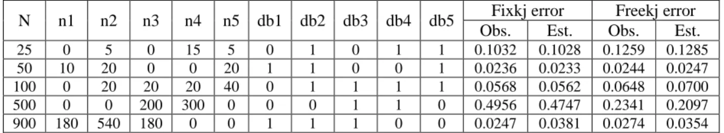
Further, we define binary variables db1 to db5 (where dbi is 0 when pi = 0 and 1 otherwise). In order

to investigating the impact of the distribution of the points regardless the sample size impact, we initially aggregate the results over all sample sizes based on the values of db1 to db5. Thirty-one sampling scheme groups (g1 to g31) were formed which are shown in Table 2-3. Each group has a

(36)

21

Table 2-3-Average calibration error as a function of the distribution of the calibration data across density(Calibration error averaged across all sample sizes and groups sorted in ascending order of average

calibration error)

Group db1 db2 db3 db4 db5 Average Error

g16 1 1 1 1 1 0.02 g3 1 0 1 0 0 0.03 g4 1 0 0 1 0 0.03 g5 1 0 0 0 1 0.03 g6 1 1 1 0 0 0.03 g7 1 1 0 1 0 0.03 g8 1 1 0 0 1 0.03 g9 1 0 1 1 0 0.03 g10 1 0 1 0 1 0.03 g11 1 0 0 1 1 0.03 g12 1 1 1 1 0 0.03 g13 1 1 1 0 1 0.03 g14 1 1 0 1 1 0.03 g15 1 0 1 1 1 0.03 g21 0 1 1 1 0 0.06 g22 0 1 1 0 1 0.07 g24 0 1 1 1 1 0.07 g19 0 1 0 1 0 0.08 g2 1 1 0 0 0 0.09 g18 0 1 1 0 0 0.10 g23 0 1 0 1 1 0.10 g17 0 1 0 0 0 0.14 g1 1 0 0 0 0 0.16 g20 0 1 0 0 1 0.20 g26 0 0 1 1 0 0.28 g25 0 0 1 0 0 0.39 g27 0 0 1 0 1 0.43 g28 0 0 1 1 1 0.45 g30 0 0 0 1 1 0.53 g29 0 0 0 1 0 0.54 g31 0 0 0 0 1 0.54

An examination of the data in Table 2-3 reveals that most of the groups with very low average calibration errors are those which have observations in bin 1 and at least one of the bins 3 to 5 (i.e. data representing both the uncongested and the congested traffic regimes). On the other hand, groups with the largest calibration errors have no observations in bins 1 and 2.

(37)

22

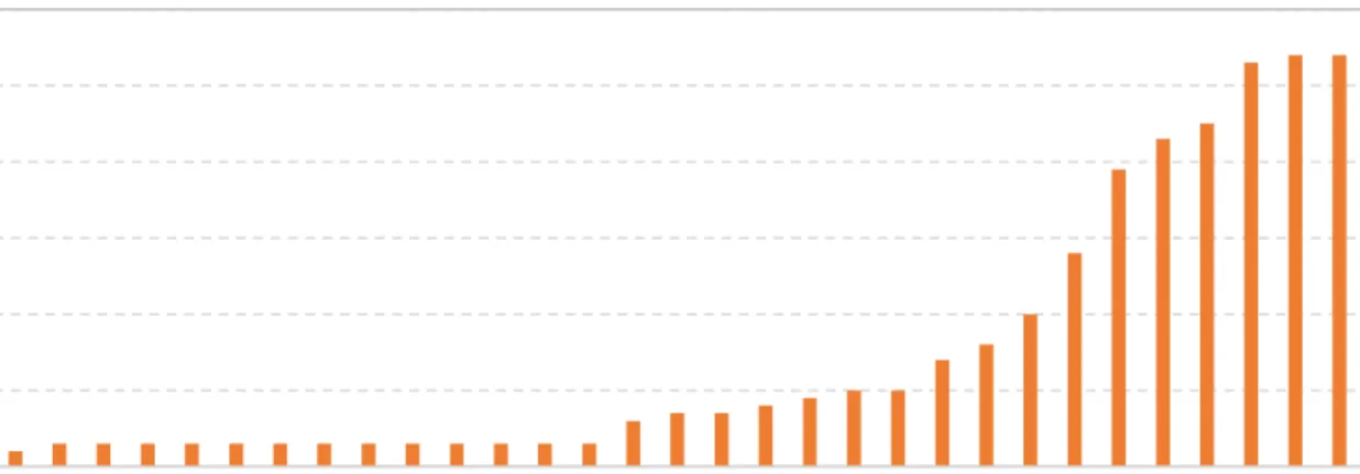
It is also instructive to examine the relative magnitude of the average calibration errors (Figure 2-4). The first set of 14 groups has very low calibration errors and the differences in the calibration errors between different groups are small. However, the last 7 groups have calibration errors as much as 25 times the calibration errors in the first set of groups. These results indicate that the distribution of the calibration data across the density has a substantial impact on the accuracy of the calibration of the macroscopic flow-speed-density model (i.e. Van Aerde’s model).

Figure 2-4- Average calibration error as a function of calibration data group number

We further aggregate the data by considering just three categories for the distribution of the calibration data:

1. Data from both the Uncongested and Congested traffic regimes, 2. Data from only the Uncongested traffic regime, and

3. Data from only the Congested traffic regime.

From the calibration of Van Aerde’s model to the population of data we have uc=76.3 (kph) and

qc=1969 (vph) and therefore the density at capacity (kc) = 25.8 (vpkpl). Density less than kc are

considered in the uncongested traffic regime and density greater than kc are considered in the congested

traffic regime. Therefore, we can classify the groups from Table 2-3 into one of the three categories identified above. Data in bin1 have density < 20 vpkpl and therefore are entirely in the uncongested regime. Data in bins 3 – 5 have density ≥ 40 vpkpl and therefore are entirely in the congested regime.

0 0.1 0.2 0.3 0.4 0.5 0.6 16 3 4 5 6 7 8 9 10 11 12 13 14 15 21 22 24 19 2 18 23 17 1 20 26 25 27 28 30 29 31 A v era g e Ca li b ra ti o n Err o r Group #

(38)

23

However, data in bin 2 span both the uncongested and congested regimes and consequently Group 17 from Table 2-3 cannot be classified. Descriptive statistics related to the calibration errors for the 30 classified groups are provided in Table 2-4. To calculate the statistics, we use the data from individual simulation runs performed in data generation section.

Table 2-4 Calibration error as a function of the distribution of the calibration data across traffic regimes

Distribution of Data Average Error Number of Groups Number of samples Standard Deviation Lower Bound at 95% CL Upper Bound at 95% CL Congested and Uncongested

Regimes 0.0512 21 118800 0.073 0.0508 0.0516

Uncongested Regime only 0.1040 2 6000 0.053 0.1027 0.1053

Congested Regime only 0.4346 7 25200 0.160 0.4326 0.4366

As is evident from Table 2-4, on average the lowest calibration errors are obtained when the calibration data represent both the uncongested and congested regimes. When the calibration data represent only the uncongested traffic regime then average calibration errors are almost double the previous category, and when the calibration data represent only the congested traffic regime, then the average calibration error is much greater. The confidence intervals of each of these categories at 95% confidence level confirms that the average errors of these categories are significantly different from each other.

2.4.2.

Investigating

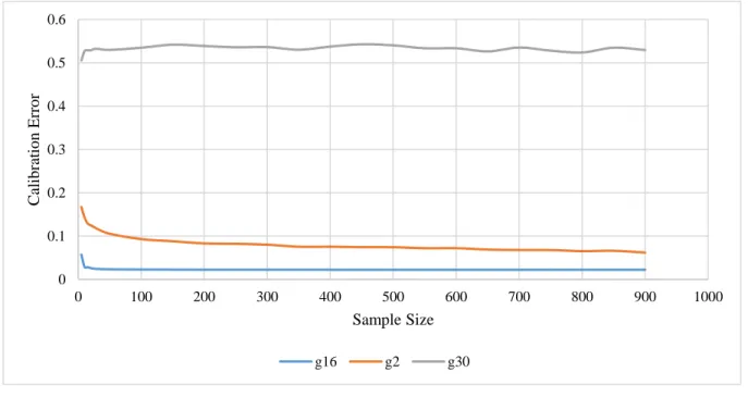
the impact of the sample size on the calibration accuracy

To understand the impact of the sample size on the estimation error, Figure 2-5 shows the calibration error as a function of sample size for three different sampling distributions, one for each of the three distributions specified at the first column of Table 2-4: group 16 as an ideal instance that have both congested and uncongested regimes; group 2 as an instance of only uncongested regimes; and group 30 as an instance of only congested regimes. We observe from Figure 2-5:

1- Sample size does not have a large impact on the calibration error when sample size exceeds 100.

2- When calibration data are from (i) uncongested and congested regimes or (ii) from the uncongested regime only, then calibration error decreases as the sample size increases.

(39)

24

However, when calibration data are from just the congested regime, calibration error appears to slightly increase as the sample size increases. We also note that in practice, it is very unlikely to have only data from the congested regime. It is much more likely to have too little (or no) data from the congested regime.

Figure 2-5-Model calibration error as a function of sample size in instances of uncongested-only (g2),

congested-only (g30), and both congested-uncongested regime (g16)

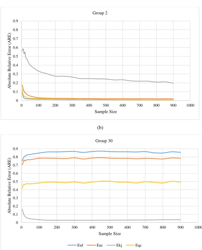
Figure 2-6 shows the estimation error of 𝜀𝑢𝑓_,_𝜀𝑢𝑐_,_𝜀𝑘𝑗_{, and}_𝜀𝑞𝑐_{(shown as Euf, etc.) in the same}

groups as Figure 2-5 (i.e. groups 16, 2, and 30). It should be noted that the parameter estimation error which is shown in Figure 2-6 is different from the errors in Table 2-3 which are the averages of the model calibration error. To compute the estimation error of traffic parameters, assume that the “true” value of each traffic stream parameter X (uf, uc, kj, qc) is 𝑋̂ and their estimated value is 𝑋̇, then the error

in the value of the traffic stream parameter is computed as:

𝜀𝑋 ₌|𝑋̂ − 𝑋̇| 𝑋̇ (2-6) 0 0.1 0.2 0.3 0.4 0.5 0.6 0 100 200 300 400 500 600 700 800 900 1000 C alib ratio n E rr o r Sample Size g16 g2 g30

(40)

25

As shown in Table 2-3, the group 16 has the lowest calibration error; therefore, we assume that the “true” values of traffic parameters (i.e. 𝑋̂) pertains to a sampling with the same distribution of the group 16. The group 16 is made by sampling equally from all density bins (i.e. bin1 to bin5). As shown in Table 2-2, bin3 has the lowest number of observations with slightly over 1000 data points; therefore, to create a base sampling we sample 1000 data points without replacement from each density bin1 to bin5 shown in Table 2-2. Then we calibrate the Van Aerde’s model on this five-thousand-point base sample to estimate the “true” parameter values. The values are: uf=126.9; uc=76.2; kj=103.4; qc=1996.

(a) 0 0.1 0.2 0.3 0.4 0.5 0.6 0.7 0.8 0.9 0 100 200 300 400 500 600 700 800 900 1000 A b so lu te R elativ e E rr o r (A R E ) Sample Size Group 16

(41)

26 (b)

(c)

Figure 2-6- Traffic parameter estimation error as a function of sample size in group 16 (a), group 2 (b), and group 30 (c) 0 0.1 0.2 0.3 0.4 0.5 0.6 0.7 0.8 0.9 0 100 200 300 400 500 600 700 800 900 1000 A b so lu te R elativ e E rr o r (A R E ) Sample Size Group 2 0 0.1 0.2 0.3 0.4 0.5 0.6 0.7 0.8 0.9 0 100 200 300 400 500 600 700 800 900 1000 A b so lu te R elativ e E rr o r (A R E ) Sample Size Group 30

(42)

27 We observe from Figure 2-6 that:

1- The estimation error of all traffic parameters generally decreases when the sample size increases for the categories that include both congested and uncongested regimes and for the categories that include uncongested-only regimes; however, the rate of the decrease of the estimation error is greater when samples sizes are relatively small (up to approximately 100 observations). For larger sample sizes, adding more observations has less impact on the estimation error.

2- When (i) the calibration data are from both the uncongested and congested regimes; and (ii) when the calibration data are from the uncongested regime only; the estimation errors for kj are much larger than the estimation errors for the other three parameters.

3- When the calibration data are only from the congested regime, then the estimation errors associated with the free speed are largest.

2.4.3.

Investigating

the impact of the sample size and the distribution of calibration data

on the accuracy of parameter estimates

Having demonstrated that calibration accuracy is highly influenced by the sample size and the distribution of the calibration data across density, we now investigate the influence that the sample size and the distribution of the calibration data across the density regime have on the accuracy of the parameter estimates.

As we observed from Figure 2-6, the estimation error (i.e. absolute relative error) for the jam density (kj) parameter is higher than for the other three traffic flow parameters in groups that include data

points from: (i) both congested and uncongested regimes (ii) uncongested-only regime. From these observations, and the expectation that in practice we most often have data from either (i) both the congested and uncongested regimes; or (ii) just the uncongested regime; it appears that the estimation errors associated with kj are most problematic. Table 2-5 shows the mean, the standard deviation, and

the coefficient of variation of the four traffic parameters estimated for: (i) two groups that only include data points from uncongested regime (i.e. groups 1, 2) (ii) two groups which have data from both congested and uncongested regimes (i.e. groups 3, 6) at the sample size of 900. The values are

(43)

28

calculated using the data of 50 replications in data generation procedure. As shown in Table 2-5, the coefficient of variation for kj parameter is significantly higher than three other parameters.

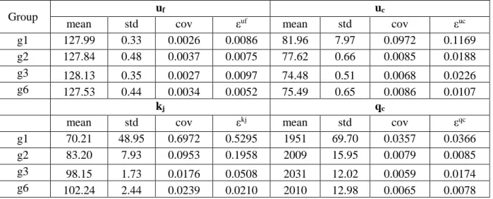
Table 2-5-Characteristics of The Estimated Traffic Flow Parameters in the Sampling Instances from Uncongested-only Regime (g1 & g2) and Both Congested-Uncongested Regimes (g3 & g6)

Group uf uc

mean std cov εuf _mean _std _cov _εuc g1 127.99 0.33 0.0026 0.0086 81.96 7.97 0.0972 0.1169 g2 127.84 0.48 0.0037 0.0075 77.62 0.66 0.0085 0.0188 g3 _128.13 _0.35 _0.0027 _0.0097 _74.48 _0.51 _0.0068 _0.0226 g6 _127.53 _0.44 _0.0034 _0.0052 _75.49 _0.65 _0.0086 _0.0107

kj qc

mean std cov εkj _mean _std _cov _εqc g1 70.21 48.95 0.6972 0.5295 1951 69.70 0.0357 0.0366 g2 83.20 7.93 0.0953 0.1958 2009 15.95 0.0079 0.0085 g3 _98.15 _1.73 _0.0176 _0.0508 ₂₀₃₁ _12.02 _0.0059 _0.0174 g6 _102.24 _2.44 _0.0239 _0.0210 ₂₀₁₀ _12.98 _0.0065 _0.0078

As shown in Table 2-5, the coefficient of variation and also the estimation error of the parameter kj is larger than of three other parameters which suggest that the estimated kj values tend to differ significantly from the true value.

To observe an instance of poorly estimated kj value, Figure 2-7 (a) shows an example of Van

Aerde’s model calibrated to a set of traffic data corresponding to Group 2 with 50 observations in the sample. Figure 2-7 (b) illustrates Van Aerde’s model calibrated on a sample of observation points of the group 16 (i.e. the group in which points are equally distributed over all five bins) when the sample size is 900.

For both graphs, the blue circles are observed speed-density points aggregated at the density bins of 0.25 vpkpl. The red line shows the calibrated Van Aerde’s model. The y-intercept of the calibrated model is the estimated free-flow speed and the x-intercept is the estimated jam density. As indicated in Figure 2-7 (a), the estimated jam density is 63 vpkpl which is significantly lower than the jam density of the comparison group (i.e. 100.7 vpkpl). This large error in estimating jam density results in large calibration error. We wish to avoid large errors in the estimates of the traffic stream characteristics

(44)

29

because these errors will undermine the credibility of the next step in the process, namely the identification of significant weather categorizations on the basis of differences between their associated traffic stream parameters values.

(a) (b)

Figure 2-7- Van Aerde’s model calibrated to uncongested data (a) and the equally distributed data (b)

2.4.4.

Improving

the robustness of calibrating kj

We hypothesize that we can make the calibration of Van Aerde’s model more robust by constraining the value that kj can assume and thereby reducing the calibration error (i.e. 𝜀𝑐) as well as the parameter

estimation errors. To examine this hypothesis, we propose a modified calibration technique compared to what has been suggested by Rakha et al. (2010), namely that the jam density is fixed at some value and the three other traffic stream parameters (i.e. uf, uc and qc) are calibrated. The jam density for a

typical freeway traffic stream is approximately 100 vpkpl (Dervisoglu et al., 2009) and therefore within the context of this study, we have fixed the jam density at 100 vpkpl. Then we repeated the method explained above by sampling from the same population as the one used above (the population with 23,370 data points). Since Figure 2-6 showed that the parameter estimation errors were less sensitive

(45)

30

to sample sizes when the sample size was larger than 100, this time we sampled at only 17 different sample size levels (i.e. 5, 10, 15, 20, 25, 30, 50, 100, 150, 200, 300, 400, 500, 600, 700, 800, 900) to reduce computational cost. Again, to maintain the randomness in the procedure, we carried out repetitions for each sample size; however, to reduce computational cost we carried out 25 repetitions rather than 50 repetitions. For each replication, we calibrated Van Aerde’s model and estimated free-flow speed, speed-at-capacity, and capacity. Also, we calculated the calibration error (𝜀𝑐_{), and absolute} relative error (𝜀𝑢𝑓_,_𝜀𝑢𝑐_{, and}𝜀𝑞𝑐_{). To distinguish these two methods, we refer to the first method in}

which all four parameters are calibrated as “free kj” and the second method, in which the value of kj is

fixed and only the other three parameters are calibrated as “fixed kj”.

Figure 2-8 compares the calibration errors from the free kj and fixed kj methods for the cases for

which all the calibration data reflects uncongested traffic conditions (i.e. group 2).

Figure 2-8- Calibration error for two calibration approaches: Freekj and Fixkj (calibration data from uncongested traffic regime only)

As shown in Figure 2-8 the calibration error when the kj is fixed is much lower than when it is free

and this is true for all sample sizes examined. This confirms our initial hypothesis that calibration errors

0 0.02 0.04 0.06 0.08 0.1 0.12 0.14 0.16 0.18 0 100 200 300 400 500 600 700 800 900 1000 C alib ratio n E rr o r Sample Size Freekj Fixkj

Using Microsimulation to Estimate the Impact of Transportation Improvements and Operational Policy Changes on Travel Time Reliability