This is a repository copy of Cloud cover effect of clear-sky index distributions and differences between human and automatic cloud observations.
White Rose Research Online URL for this paper: http://eprints.whiterose.ac.uk/110263/
Version: Accepted Version
Article:
Smith, CJ orcid.org/0000-0003-0599-4633, Bright, JM and Crook, R (2017) Cloud cover effect of clear-sky index distributions and differences between human and automatic cloud observations. Solar Energy, 144. pp. 10-21. ISSN 0038-092X
https://doi.org/10.1016/j.solener.2016.12.055
© 2017 Elsevier Ltd. Licensed under the Creative Commons Attribution-NonCommercial-NoDerivatives 4.0 International http://creativecommons.org/licenses/by-nc-nd/4.0/
[email protected] https://eprints.whiterose.ac.uk/ Reuse
Unless indicated otherwise, fulltext items are protected by copyright with all rights reserved. The copyright exception in section 29 of the Copyright, Designs and Patents Act 1988 allows the making of a single copy solely for the purpose of non-commercial research or private study within the limits of fair dealing. The publisher or other rights-holder may allow further reproduction and re-use of this version - refer to the White Rose Research Online record for this item. Where records identify the publisher as the copyright holder, users can verify any specific terms of use on the publisher’s website.
Takedown
If you consider content in White Rose Research Online to be in breach of UK law, please notify us by
Cloud cover effect of clear-sky index distributions and differences
between human and automatic cloud observations
Christopher J. Smitha,b,∗, Jamie M. Brighta, Rolf Crooka a
Energy Research Institute, School of Chemical and Process Engineering, University of Leeds, Leeds LS2 9JT, UK
b
Institute for Climate and Atmospheric Science, University of Leeds, Leeds LS2 9JT, UK
Abstract
The statistics of clear-sky index can be used to determine solar irradiance when the theoretical clear sky irradiance and the cloud cover are known. In this paper, observations of hourly clear-sky index for the years of 2010–2013 at 63 locations in the UK are analysed for over 1 million data hours. The aggregated distribution of clear-sky index is bimodal, with strong contributions from mostly-cloudy and mostly-clear hours, as well as a lower number of intermediate hours. The clear-sky index exhibits a distribution of values for each cloud cover bin, measured in eighths of the sky covered (oktas), and also depends on solar elevation angle. Cloud cover is measured either by a human observer or automatically with a cloud ceilometer. Irradiation (time-integrated irradiance) values corresponding to human observations of “cloudless” skies (0 oktas) tend to agree better with theoretical clear-sky values, which are calculated with a radiative transfer model, than irradiation values corresponding to automated observations of 0 oktas. It is apparent that the cloud ceilometers incorrectly categorise more non-cloudless hours as cloudless than human observers do. This leads to notable differences in the distributions of clear-sky index for each okta class, and between human and automated observations. Two probability density functions—the Burr (type III) for mostly-clear situations, and generalised gamma for mostly-cloudy situations—are suggested as analytical fits for each cloud coverage, observation type, and solar elevation angle bin. For human observations of overcast skies (8 oktas) where solar elevation angle exceeds 10◦, there is no significant difference between the
observed clear-sky indices and the generalised gamma distribution fits.
Keywords: clouds, clear-sky index, statistics, ceilometer
∗Corresponding author
Email addresses: [email protected](Christopher J. Smith),[email protected](Jamie M. Bright),[email protected](Rolf Crook)
Acronyms
AERONET Aerosol Robotic Network
AFGL Air Force Geophysics Laboratory BADC British Atmospheric Data Centre BSRN Baseline Surface Radiation Network CDF Cumulative Distribution Function DNI Direct Normal Irradiance
ECMWF European Centre for Medium-range Weather Forecasts GHI Global Horizontal Irradiance
GLOMAP Global Model of Aerosol Processes
IGBP International Geosphere–Biosphere Programme MIDAS Met Office Integrated Data Archive System PDF Probability Density Function
RMSE Root Mean Square Error RO Global Radiation Observations UKMO UK Meteorological Office UTC Coordinated Universal Time WH UK Hourly Weather Observations 1. Introduction
1
The most reliable way to determine the solar resource for a particular location, assuming
2
there have been no detectable effects of climatic change, is to set up long-term pyranometer
3
observations. For many sites of interest, pyranometer records are not frequently obtained for
4
a sufficiently long period prior to installation of a solar energy system (Gueymard and Wilcox,
5
2011). Other meteorological variables such as sunshine hours (˚Angstr¨om, 1924; Muneer et al.,
6
1998; Prescott, 1940), diurnal temperature range (Bristow and Campbell, 1984; de Jong and
7
Stewart, 1993; Hargreaves et al., 1985; Supit and van Kappel, 1998), precipitation (de Jong and
8
Stewart, 1993), cloud type (Kasten and Czeplak, 1980; Matuszko, 2012) and fractional cloud
9
cover (Brinsfield et al., 1984; Kasten and Czeplak, 1980; Matuszko, 2012; Muneer and Gul,
10
2000; Nielsen et al., 1981; Supit and van Kappel, 1998; W¨orner, 1967) can be used to estimate
11
solar irradiance. Temperature, pressure, cloud cover, cloud type, rainfall and sunshine hours
12
are routinely measured at weather stations globally.
13
Since clouds are the largest attenuating factors of solar irradiance in large areas of the globe
14
(Wacker et al., 2015), cloud cover is a useful predictor of solar resource (Kasten and Czeplak,
15
1980). If the sky is cloudless, irradiance can be predicted from the solar geometry, surface
16
albedo, and optical properties of aerosols, ozone and water vapour using a radiative transfer
17
calculation (M¨uller et al., 2012). Alternatively, several clear-sky models exist in the literature
18
which are empirical relationships between one or more of these atmospheric variables (or of
Nomenclature
a Probability distribution scale parameter
c Burr (type III) distribution shape parameter
d Generalised gamma distribution shape parameter
ei Expected frequency of clear-sky index observations
G surface global horizontal irradiation (J m−2)
G0 top-of-atmosphere global horizontal irradiation (J m−2)
Gcs clear sky surface global horizontal irradiation (J m−2)
k Burr (type III) distribution shape parameter
Kc clear-sky index
KT clearness index
N cloud cover (oktas)
oi Observed frequency of clear-sky index observations
p Generalised gamma distribution shape parameter Γ(·) Gamma function
θe solar elevation angle,◦
χ2 Goodness-of-fit statistic
their derived quantities) and clear-sky irradiance (Gueymard, 2012). When clouds are present,
20
the fraction of time clouds obscure the sun, the optical thickness of the clouds, and secondary
21
effects such as reflections from cloud sides and between cloud layers, can all have important
22
effects on the proportion of irradiance that reaches the surface. Cloud transmission is therefore
23
the most uncertain component of surface irradiance in most locations.
24
Typically, cloud cover is recorded at meteorological stations as an integer number of oktas,
25
here denoted N, which is the number of eighths of the sky obscured by clouds (Met Office,
26
2010). An additional okta code 9 is used for situations where the sky is obscured by fog, haze
27
or other meteorological phenomena. For human observations, a convention is to reserve 0 oktas
28
for completely cloudless sky and 8 oktas for completely overcast sky, so the limits of 1 okta and
29
7 oktas are extended to almost clear and almost overcast respectively (Jones, 1992). In some
30
automated algorithms a different convention may be followed, for example recording up to 1/16
31
cloudiness as 0 oktas and greater than 15/16 cloudiness as 8 oktas (Wacker et al., 2015).
32
Clear-sky index,Kc =G/Gcs, estimates atmospheric attenuation due to clouds by measuring
33
the ratio of surface solar irradiance or irradiationGto the corresponding amount that would be
34
received under a clear (cloudless) sky, Gcs. It also accounts for the influence of surface albedo.
35
Other cloudless-sky attenuators such as water vapour, ozone and aerosols are retained in the
36
calculation of Gcs. The clear-sky index is less dependent on airmass than the commonly used
37
clearness index KT = G/G0, where G0 is top-of-atmosphere solar irradiance. Some authors
have worked to reduce this dependence by introducing a rescaling of the clearness index, to
39
either map the observed range of clearness indices into the interval 0–1 for each solar elevation
40
angle class (Olseth and Skartveit, 1987) (i.e. a normalised clearness index), or to adjust for
41
airmass based on clear-sky Linke turbidity values (Perez et al., 1990).
42
Previous relationships between N and KT, Kc, or G, have tended to provide a
one-to-43
one correspondence between N and the variable of interest (Brinsfield et al., 1984; Kasten
44
and Czeplak, 1980; Matuszko, 2012; Muneer and Gul, 2000; Nielsen et al., 1981; Supit and
45
van Kappel, 1998; W¨orner, 1967). On the other hand, several authors have described the
46
distributions of clearness or clear-sky index parameterised by its longer-term mean (Bendt et al.,
47
1981; Graham and Hollands, 1990; Graham et al., 1988; Hollands and Suehrcke, 2013; Jurado
48
et al., 1995; Liu and Jordan, 1960; Olseth and Skartveit, 1984, 1987; Suehrcke and McCormick,
49
1988) or by airmass (Moreno-Tejera et al., 2016; Tovar et al., 1998). We aim to bring these parts
50
together by reporting clear-sky index distributions for each N class, and secondarily binned by
51
solar elevation angle. A simplified distributional approach was provided by the authors in
52
Bright et al. (2015) for clear sky and 6, 7 and 8 oktas to estimate cloud transmission in
sun-53
obscured minutes and clear breaks, but did not group observations into human and automatic
54
cloud retrievals or elevation angle bins, which as will be shown is important.
55
The hourly statistics of clear-sky index grouped by N and solar elevation angle would be
56
useful in situations where long-term irradiation data were not available, but measurements of
57
hourly N were (assuming the hourly solar elevation angle was known or could be determined).
58
The probability of transitioning from one N state to the next N state can then be simulated
59
with a Markov chain model (e.g. Bright et al. (2015); Ehnberg and Bollen (2005)), and the
60
cloud transmission for each hour selected as a random variable from each Kc distribution for
61
that N class.
62
2. Determining the clear-sky index 63
2.1. Relationships between clear-sky index and cloud cover
64
Kasten and Czeplak (1980) found an empirical relationship between hourly Kc and hourly
65
N using 10 years of data for Hamburg, Germany, for solar elevation angles above 5◦: 66
Kc = 1−0.75(N/8)3.4
where the clear-sky irradiance [W m−2] is modelled as 67
Gcs = 910 sinθe−30. (2)
where θe is solar elevation angle in degrees. The attenuation coefficient of 0.75 in eq. (1) is
68
an overall average over all cloud types, and varies from 0.39 for cirriform clouds to 0.84 for
69
nimbostratus. This relationship was later found to be valid for 5 UK sites by Muneer and Gul
70
(2000), where slightly better fits can be obtained by tuning coefficients for each site. Other,
71
more complex relationships for Gas a function of cloud cover were developed by Nielsen et al.
72
(1981) and Brinsfield et al. (1984). Matuszko (2012) tabulated observed 10-minutely irradiance
73
by okta class and solar elevation angle band for Krakow, Poland.
74
Cloud cover can indicate how likely it is that the sun is obscured by clouds (e.g. Muneer
75
and Gul (2000)). It does not however provide any information as to how opaque the clouds
76
are to solar irradiance. Clear-sky index can take a wide variety of values for each N class. For
77
example, a sky could be overcast (N = 8) with thin cirrus clouds or thick nimbostratus clouds.
78
In this case, Kc has been observed to vary from 0.07 for overcast nimbostratus to 1.00 for
79
overcast cirrus (Matuszko, 2012). Kasten and Czeplak (1980) reported long-term averages of
80
0.16 for nimbostratus and 0.61 for cirriform clouds. Although Brinsfield et al. (1984) considers
81
opaque clouds in their formulations, the various optical depths of both translucent and opaque
82
clouds that are observed may still produce a distribution of results. As shown in Bright et al.
83
(2015), the distributions of Kc for 6, 7 and 8 oktas can take a wide range of values. For these
84
reasons, the distributional spread ofKc for a particular cloud coverage of N oktas can be more
85
useful than its mean or median value.
86
2.2. Observational data
87
The meteorological observations of cloud cover and solar irradiation are taken from four
88
years (2010–2013) of the network of UK Met Office Integrated Data Archive System (MIDAS)
89
stations (Met Office, 2012). Several datasets are available to registered users at the British
90
Atmospheric Data Centre (http://badc.nerc.ac.uk). The UK Hourly Weather Observation
91
data (WH) and Global Radiation Observations (RO) were used. Included within the WH data,
92
amongst several other meteorological variables, are observations of hourly N, and whether the
1395 1415 1285 1302 842 862 779 30620 811 1198 19206676 692 461 708 726 440 775 1161 1190 669 643 19187595 556 583 395 1046 1145 1144 57199 55511 17314 533 384 370 1568 57063 56963 1450 1467 1033 1023 1083 315 18974 105 1007 24125 212 19260 235 268 177 54 67 44 79 113 132 23 161 9
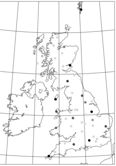
Figure 1: MIDAS stations that provide quality-controlled hourly irradiation and cloud cover observations for 2010–2013. Station numbers refer to MIDAS station IDs. The strength of shading indicates the proportion of observations that were observed by a human (15% grey corresponds to 0% human observations, scaling linearly to 100% black representing 100% human observations). The lines of longitude and latitude mark the boundaries of each GLOMAP aerosol climatology grid cell.
observation was automatic or human-observed. The hourly irradiation G is taken from the
94
RO data. Both datasets indicate the date and time of the observation and the station ID
95
code. Data were used when observations of G and N exist for the same station and hourly
96
timestamp, and both pass internal Met Office quality control checks as indicated by state flags
97
for each observation. An additional screening procedure was implemented to remove duplicate
98
observations. One station contained only two hours of valid data for the four years, and this
99
station was also disregarded. Further checks removed observations with unrealistically high
100
clearness index values as described in section 2.4.5. A total of 1,121,334 hourly observations
101
were retained from 63 MIDAS stations across the UK. The locations of these stations are shown
102
in fig. 1.
2.3. Cloud cover observational practice
104
Cloud cover observations can either be made by a human observer or a cloud ceilometer,
105
which uses a laser to detect cloud bases automatically (WMO, 2014). In recent years, the
106
UK Met Office has moved towards fully automated weather measurements at most stations,
107
but human observers are still present at some research stations and airfields during operational
108
hours1. This reflects observational practice in many other countries (Dai et al., 2006; Perez et al.,
109
2001; Wauben et al., 2006). A previous study has found that human and automated methods
110
can produce quite different results, with agreements in N between human and automated
111
observations occurring for 39% of hours and agreements within ±2 oktas occurring for 88% of 112
hours in the Netherlands (Wauben et al., 2006). Wacker et al. (2015) found that ceilometer
113
observations of cloud cover tend to be biased low compared to those observed by a human in
114
Switzerland. A human observer typically makes a subjective judgement of the cloud-obscured
115
proportion of the entire visible sky dome at the end of a reporting period (e.g. every hour in
116
the WH data), while a cloud ceilometer consists of a zenith-pointing device that records the
117
amount of time that a laser beam was intercepted by clouds divided by the length of the period
118
(Dai et al., 2006).
119
The solar irradiation data collected by MIDAS stations are hourly totals. Solar irradiation
120
is measured using Kipp & Zonen CMP10 and CMP11 pyranometers, with cleaning,
level-121
checking and recalibration performed on a regular basis including at fully automated sites2 . As
122
irradiation is recorded hourly, there can be a timing mismatch between the dominant conditions
123
of the hour and the cloud amount recorded at the end of the hour by a human observer if clouds
124
accumulate or disperse during the hour. The automatic ceilometer method assumes that the
125
clouds overpassing the zenith during the hour are representative of the entire sky conditions,
126
which are not always case if clouds are localised in one part of the sky, giving a spatial mismatch
127
between recorded clouds and actual cloud cover. Furthermore, thin cloud is sometimes not
128
detected by the laser and fog can be mistaken for low-level overcast conditions. The distinction
129
of whether an observation was made by a human or was automatic is an important one and is
130
taken into account in the analysis.
131
1
Personal communication with a member of the British Atmospheric Data Centre team.
2
2.4. Generation of clear sky solar irradiance
132
For this study, Gcs is simulated using a radiative transfer simulation with prescribed
atmo-133
spheric constituents. The advantages of this are that climatological values of the main clear-sky
134
solar attenuators can be input into the model to quickly generate an estimate of clear-sky
ir-135
radiance that is location- and month-dependent. For 0 oktas, this also gives an indication of
136
natural variability in atmospheric transmission of clear skies around the climatological mean
137
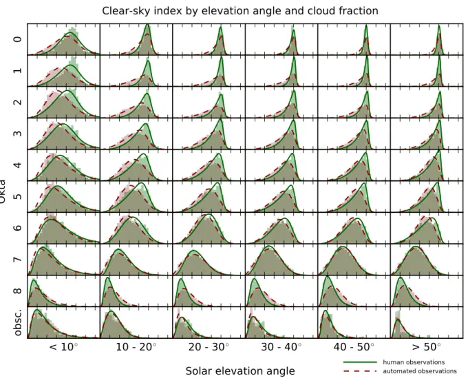
value. A further reason for this approach that is shown in section 3 is that the cloud cover
ob-138
servation method (human or automated) determines the shape of each cloud cover observation
139
bin, including 0 oktas.
140
2.4.1. Atmosphere
141
The two-stream solution to the discrete-ordinate radiative transfer method (Kylling et al.,
142
1995), implemented in the libRadtran software package (Mayer and Kylling, 2005), is used to
143
calculate clear-sky irradiance. The background atmosphere for mixed gases concentration is
144
provided by the Air Force Geophysics Laboratory (AFGL) mid-latitude summer atmosphere
145
for April–September and mid-latitude winter for October–March (Anderson et al., 1986). Air
146
temperature, and ozone and water vapour mass mixing ratios, on 60 model levels for each
147
month of 2010–2013 from the European Centre for Medium-range Weather Forecasts (ECMWF)
148
ERA-Interim reanalysis data, provide the climatological atmospheric conditions. These data
149
are taken on a spatial grid of 1.5◦ ×1.5◦. A pseudo-spherical correction is implemented in 150
the radiative transfer code, which accounts for the curvature of the earth’s atmosphere and
151
improves the accuracy of clear-sky irradiance calculations at low sun.
152
2.4.2. Aerosols
153
Aerosols are highly spatially and temporally variable and may lead to the highest uncertainty
154
in the calculated clear-sky irradiance values. Point measurements of aerosol conditions are made
155
by the AERONET network, but are only possible under favourable conditions and some sites
156
experience several months without a valid observation. Another technique considered was to
157
estimate aerosol conditions based on retrieved values of horizontal visibility from the WH data,
158
but this was found to consistently underestimate clear-sky irradiance and actually increased,
159
rather than reduced, the ranges of Kc observed. Therefore, aerosol optical properties are taken
160
from the Global Model of Aerosol Processes (GLOMAP) model (Scott et al., 2014; Spracklen
et al., 2005), which provides aerosol optical depth, single scattering albedo and asymmetry
162
factor in 6 solar shortwave bands on 31 atmospheric levels for each month. The native GLOMAP
163
spatial grid of 2.8◦×2.8◦ is used without interpolation, which divides the UK into 11 aerosol 164
zones (shown in fig. 1).
165
2.4.3. Surface albedo
166
Surface albedo from the International Geosphere-Biosphere Programme (IGBP) library at
167 a resolution of 1 6 ◦ × 1 6 ◦
has been used (Belward and Loveland, 1996). One issue with using
168
the same surface type for the full year may be to underestimate the albedo from snow-covered
169
surfaces in winter. Radiative transfer simulations performed by the authors suggest that a
170
perfectly reflecting surface predicts about 13% higher downwards irradiance than a perfectly
171
absorbing surface due to multiple reflections between atmosphere and the ground under clear
172
sky. This result is consistent for all solar elevation angles. Real surfaces are not totally absorbing
173
and snow-covered surfaces are not totally reflective. The errors introduced for global horizontal
174
radiation (GHI) by using an incorrect surface albedo are therefore likely to be smaller than 13%
175
under clear sky conditions. The overall impact is expected to be small as this phenomenon will
176
only affect a few winter days each year.
177
2.4.4. Solar position
178
To match the clear-sky simulation to observation as accurately as possible, an accurate
179
representation of solar elevation angle is required. Met Office data recording conventions state
180
that the observation recorded for each UTC hour (SYNOP climate message) is taken 10 minutes
181
before the hour (Met Office, 2015a). For solar irradiation (HCM climate message), the time
182
period of data collection runs from 70 minutes to 10 minutes before the observation time stamp
183
(at the end of every UTC hour). libRadtran provides the Blanco-Muriel et al. (2001) algorithm
184
for calculating solar elevation angle, which provides long-term accuracy for solar elevation
185
within 0.1◦. The effective solar elevation angle is calculated centred at 40 minutes prior to 186
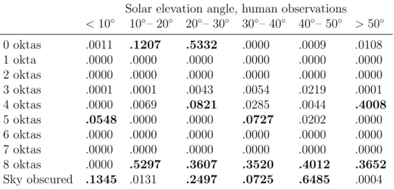
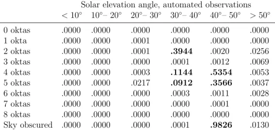
each hour of each day at each MIDAS station by taking a sum of 61 minutely samples of the
187
solar elevation angle between 70 and 10 minutes before the observation time stamp, inclusive.
188
Solar elevation angles below 0◦ are excluded from the sum, and the sum of the minutely sines 189
of elevation angle are divided by the number of minutes in which the sun is above the horizon
190
to obtain the effective sine of elevation angle. This calculation is again performed internally in
libRadtran.
192
This procedure of obtaining an effective solar elevation angle corresponds to practice A3 of
193
Blanc and Wald (2016). It is found that this practice predicts direct normal irradiance (DNI)
194
with a RMSE of 4% for all elevation angles and 24% for elevation angles below 15◦ (Blanc 195
and Wald, 2016) at the high-quality BSRN site at Payerne, Switzerland. This is better than
196
assuming that the elevation angle corresponding to the middle of the hour is representative,
197
however a more accurate practice (A5) involves taking the inverse sine of the ratio of direct
198
horizontal irradiation to direct normal irradiation (Blanc and Wald, 2016). This practice has
199
not been implemented in this work as the hourly DNI is not available in libRadtran.
200
2.4.5. Additional quality control check
201
After calculatingKc and obtaining θefor each valid hour, an additional screening procedure
202
was implemented to remove all observations where the clearness indexKT exceeded 0.85. This
203
is on the basis that hourly clearness indices exceeding 0.85 are very rarely, if ever, observed
204
in high-quality data (NREL, 1993; Vignola et al., 2012). This additional constraint excluded
205
0.34% of observations, the majority of which were at very low elevation angles where small
206
errors in the calculated solar position can cause large errors in the ratios of Kc and KT.
207
3. Distributions of clear-sky index 208
3.1. Aggregated observations
209
Figure 2 shows the overall distribution of clear-sky index from all 63 weather stations in
210
all cloud conditions. The distribution is bimodal with contributions from cloudless hours near
211
Kc = 1 and cloudy hours near Kc = 0.3. There are a lower number of observations for
212
intermediate clear-sky indices. Bimodal behaviour for hourly normalised (scaled to the range
213
0–1) clearness index observations has been observed in Norway and Vancouver (Olseth and
214
Skartveit, 1987), and it is reasonable to expect a similar pattern for clear-sky index would also
215
occur in the similar maritime climate of the UK. The clear sky mode at Kc = 1 shows that
216
the radiative transfer simulation with prescribed albedo, aerosol, H2O and O3 climatologies
217
provides a good estimate of irradiation in cloudless skies.
218
There are a number of observations from hours where Kc is much larger than 1 indicating
219
significantly more solar irradiation than would be expected under cloudless conditions for a
0.0 0.5 1.0 1.5 2.0 Clear-sky index 0.0 0.2 0.4 0.6 0.8 1.0 1.2 1.4 Frequency density
number of hours, despite rejection of values where KT >0.85. For hourly data, it is expected
221
that the averaging time would cause short-term cloud enhancement effects to cancel out. It is
222
however possible that cloud enhancement effects could influence the hourly Kc value if clouds
223
tend to group in, or avoid, one region of the sky due to geographical features, such as mountains
224
or coastlines.
225
3.2. Distribution by solar elevation angle
226
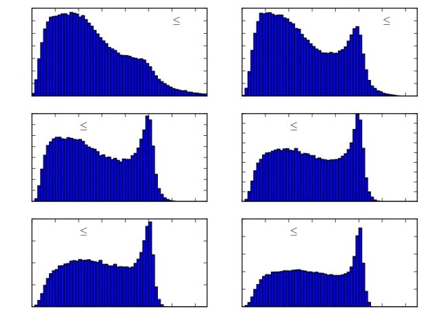
In fig. 3, the clear-sky index histograms are grouped into bins of elevation angle from 0–10◦, 227
10–20◦and so on up to the top group of 50–63◦. These histograms reveal different characteristics 228
of the clear-sky index distribution in each elevation angle bin. The θe ≤ 10◦ bin is unimodal 229
showing the greatest accumulation of Kc values around 0.3–0.4. The spread of values is the
230
largest for any solar elevation class, and this group is also responsible for a large majority of
231
the extremely high, Kc >1.2, observations. For the 10◦ < θe ≤20◦ bin, the bimodal shape of 232
the distribution starts to become apparent. Low Kc values are still more common, and there
233
is a lower frequency of extremely high observations. As elevation angle increases, the Kc ≈ 1
234
“spike” of the distribution becomes sharper and higher than the low Kc “hump”, which starts
235
to flatten out and become more uniform, and instances of Kc >1.2 virtually disappear. In the
236
top elevation angle group the greatest value of Kc barely exceeds 1.1.
237
It is therefore shown that highKc values are more likely to occur at low solar elevation angle
238
bins, and that Kc is not independent of solar elevation angle for the choices of inputs used in
239
the radiative transfer model. There are several reasons why a large spread, including some very
240
large, Kc values can occur for θe ≤ 10◦. At low sun under scattered clouds, reflections from 241
the undersides of clouds can enhance diffuse irradiance, or clouds near the horizon in the solar
242
direction can forward-scatter sunlight. If this happens due to clouds preferentially grouping in
243
one part of the sky, this may lead to consistently highKc values for low solar elevation angles as
244
a result of non-cancelling cloud enhancement effects. The effect of snow in winter and how this
245
enhances surface clear-sky irradiance has been described previously. Under clouds, multiple
246
reflections between snow-covered ground and cloud bases may enhance irradiance under all-sky
247
conditions, and this effect may be greater than the 13% calculated for clear-sky conditions. One
248
reason for the lack of high Kc spike is that where clouds are present, transmitted irradiance
249
may be lower at low solar elevations as both solar beam path through the cloud is longer, and
0.0 0.2 0.4 0.6 0.8 1.0 1.2 1.4 0.0 0.2 0.4 0.6 0.8 1.0 1.2 1.4 0◦ <θ e 10◦ 0.0 0.2 0.4 0.6 0.8 1.0 1.2 1.4 0.0 0.2 0.4 0.6 0.8 1.0 1.2 1.4 10◦ <θ e 20◦ 0.0 0.2 0.4 0.6 0.8 1.0 1.2 1.4 0.0 0.2 0.4 0.6 0.8 1.0 1.2 1.4 1.6 20◦ <θ e 30◦ 0.0 0.2 0.4 0.6 0.8 1.0 1.2 1.4 0.0 0.2 0.4 0.6 0.8 1.0 1.2 1.4 1.6 1.8 30◦ <θ e 40◦ 0.0 0.2 0.4 0.6 0.8 1.0 1.2 1.4 0.0 0.5 1.0 1.5 2.0 40◦ <θe 50◦ 0.0 0.2 0.4 0.6 0.8 1.0 1.2 1.4 0.0 0.5 1.0 1.5 2.0 2.5 50◦ <θe 63◦ Clear-sky index Frequency density
θe = 60°
θe = 15°
(a)
(b)
Figure 4: Schematic of cloud shading for the same (fictional) cloud for solar elevation angle of (a) 60◦ and (b)
15◦. Both the shaded area (light grey) and the maximum path length of the solar beam (arrow through cloud)
increases at low solar elevation angles.
cloud shadows project a greater area (fig. 4). None of these effects are sources of error and
251
represent real-world phenomena; they must therefore be included in the distributions.
252
Extreme high values of Kc could also be due to errors either in measurement or
calcula-253
tion. DNI reported by pyranometers becomes less reliable at low solar elevations due to cosine
254
response errors (Vignola et al., 2012). When generating Kc values, the hourly sine-weighted
255
mean elevation angle may not be adequately representative of all conditions during the hours
256
of sunrise and sunset. Furthermore, UK Met Office practice of recording measurements at 10
257
minutes before the hour may not have been observed at all stations, or errors in the clock time
258
at the MIDAS site may be present3. Large differences between sinθe at the start and end of the
259
hour can account for this. Although the pseudo-spherical correction for the curvature of the
260
earth’s atmosphere is made in the radiative transfer code, all instances whereθe<0◦ are set to 261
zero in the hourly averaging of zenith angle. In reality a small amount of diffuse irradiance at
262
dusk and dawn is present and would contribute to the total received by a pyranometer. Finally,
263
the impact of horizon obstructions can cause instances of otherwise clear sky receiving a low
264
Kc value.
265
3
The datasets were originally analysed without the 10-minute offset where it was observed that the distribu-tional spread was much greater, indicating that the practice has been implemented at the majority of MIDAS stations if not all.
54 67 44 79 113 132 23 161 9 18974 105 1007 24125 212 19260 235 268 177 1568 57063 56963 1450 1467 1033 1023 1083 315 1046 1145 1144 57199 55511 17314 533 384 370 1161 1190 669 643 19187 595 556 583 395 1198 19206 676 692 461 708 726 440 775 1395 1415 1285 1302 842 862 779 30620 811 East → No rt h →
Clear-sky index distributions for 63 UKMO MIDAS stations
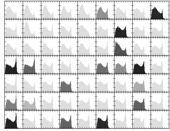
Figure 5: Histograms of Kc for each individual MIDAS station. The shading of the histogram denotes the
proportion of human observations, with light (15%) grey denoting fully automated and black denoting fully human-observed. The x-axis runs from 0 to 1.6 with tick intervals of 0.2 and the y-axis is the probability density running from 0 to 2 in tick intervals of 0.5. Station ID numbers are in the top-right of each histogram. For station locations, refer to fig. 1.
3.3. Distribution by MIDAS weather station
266
Owing to the influence of weather systems from the Atlantic and the rain-shielding effect
267
of hills and mountains such as the Pennines, the western side of the British Isles typically
268
experiences more rainfall than the eastern side (Met Office, 2015b). To investigate whether
269
this pattern is prevalent in cloud transmission, the Kc distribution from each of the 63 MIDAS
270
stations in fig. 1 is investigated individually.
271
The 63 stations are grouped into a 7×9 grid by sorting the station latitudes in order from
272
south to north and then from west to east across each band. In fig. 5, the distribution ofKc for
273
each weather station is shown. The proportion of human observations at each station is denoted
274
by the strength of the shading. A total of 17 stations have at least some human observations,
275
ranging from 19% to 99% of the total for that station.
276
Most individual stations exhibit the bimodal characteristic of clear-sky index that is a
feature of the aggregated distribution in fig. 2. Some individual stations, typically located in
278
Scotland and Northern Ireland, have a low or non-existent clear-sky spike showing a tendency
279
for cloudiness. From south to north, there is a slight trend for a decrease in overall cloud
280
transmission by comparing the frequency densities of the low Kc humps, but this varies from
281
station to station, and could be an consequence of the annually averaged lower solar elevation
282
angles at these latitudes. There does not appear to be an overall trend in the west to east
283
direction. It should be borne in mind that differences in instrumental response and local
284
microclimates may affect the Kc values produced from individual stations. On the whole,
285
there are no clear systematic differences between stations by observation method for total Kc
286
distributions.
287
3.4. Distribution of cloud cover by solar elevation angle
288
The differences in the shape of the Kc distributions for each elevation angle bin could be
289
an indication of generally fairer weather conditions at higher solar elevation angles, or could
290
be a result in the reduction of the variance in Kc values in genuinely clear hours that cause
291
observations to contract towardsKc = 1. The cloud cover habits for each elevation angle class
292
have been investigated. It is confirmed that clearer conditions are not generally more likely at
293
higher solar elevation angle bins as shown in fig. 6.
294
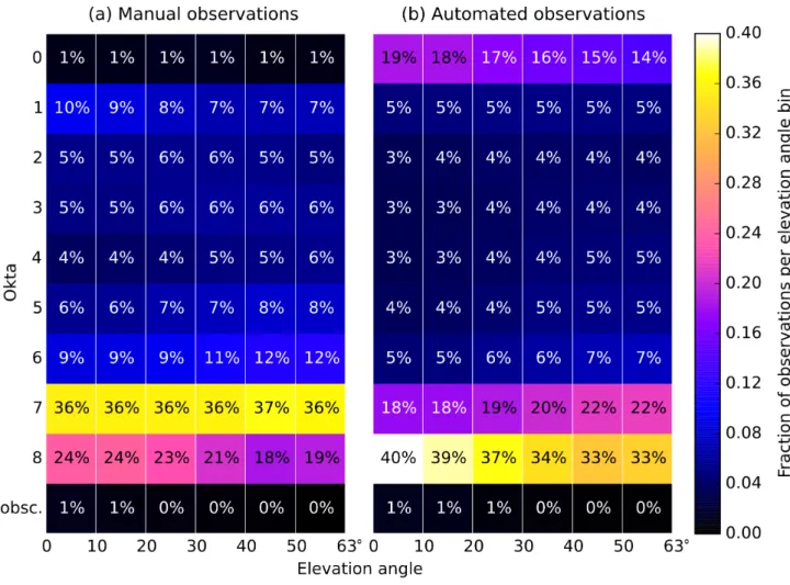
Figure 6 shows there is a significant difference between cloud cover reporting for the human
295
and automatic methods across all solar elevation angles. Automated cloud systems are much
296
more likely (14–19% of hours) to record 0 oktas than human observers (1% of hours). There
297
is also a tendency for the automated recording system to record 8 oktas more commonly than
298
the human observers (33–40% of the time compared to 19–24%). For both 8 oktas and 0 oktas,
299
there is an elevation angle dependency for automated observations, with these classes more
300
likely to be recorded at lower elevation angle bins. For human observations, this pattern is seen
301
with 1 okta and 8 oktas. Conversely, for human observers 7 oktas is most commonly recorded
302
with 36% or 37% of observations (no detectable elevation angle dependency), whereas 7 oktas
303
is recorded only 18–22% of the time in the automated observations, increasing with elevation
304
angle. Intermediate (1 ≤ N ≤ 6) cloudiness is more likely to be noted by human observers
305
across all elevation angle bins. The differences in N frequency between the two methods may
306
be partially due to the recording convention for human observers of 0 oktas representing totally
Figure 6: Heat map of okta frequency count for each elevation angle bin for (a) human and (b) automated cloud cover observations. Percentages and shading colour relates to the fraction of each elevation angle class (column) assigned to each cloud okta class. Columns may not sum to 100% due to rounding.
cloudless skies and 8 oktas representing fully overcast skies. Any cloud presence, however small,
308
should be recorded as 1 okta, and likewise a small break in an otherwise overcast sky should
309
be recorded as 7 oktas. It is unlikely that a ceilometer would “hit” a small isolated cloud or
310
cloud-break over the course of an hour, therefore classifying more “true” 1 okta hours as 0
311
oktas, and “true” 7 okta hours as 8 oktas.
312
The lack of Kc ≈ 1 spike for the θe ≤ 10◦ bin is unlikely to be due to significantly higher 313
cloudiness for these observations in both the human-observed and automated cases. Separate
314
analysis shows that the seasonal distribution shapes are similar to the annual ones in fig. 3, with
315
a slightly greater tendency to lowKc values in winter where okta 8 is observed more frequently.
316
3.5. Distribution by okta and elevation angle
317
The distributions at each okta class were subdivided by elevation angle group (fig. 7),
318
with separate results provided for human and automated observations. It is seen that this
319
division is a necessary one, particularly at low okta classes. The 0 oktas distribution for human
observations is slightly left-skewed at low solar elevation angles, becoming more symmetric
321
aroundKc = 1 at higher elevations. In contrast, the histograms of automated observations for
322
0 oktas exhibit more left skew that does not vanish at the highest elevation angle class. This
323
implies that humans are more able to detect cases of genuine clear sky and that the spatial
324
mismatch between the observation ofN by the ceilometer and the rest of the sky is more serious
325
than the temporal mismatch of N recorded by a human at the end of the hour and irradiance
326
measured over the course of the hour. For automated observations, it is clear that a significant
327
number of hours that are not cloudless are being reported as 0 oktas. This results in the left
328
skew present at 0 oktas and the heavier weight of the left tails for 1–3 oktas compared to the
329
human observations. The left-skew for 0 oktas is still present for human observations, albeit
330
smaller.
331
When cloud coverage is between 1 and 6 oktas, more of the mass of the distributions
332
are located to the left for automated observations than for human observations in all solar
333
elevation angle bins. This indicates that the automatic method tends to attribute cloudier
334
observations to a particular okta value than a human would for intermediate cloudiness. The
335
7 okta distributions are roughly similar to first order. However, a large difference occurs in
336
“overcast” skies (8 oktas), where humans tend to record a greater proportion of low Kc hours
337
than the ceilometer. This would suggest that humans are generally more able to correctly
338
identify genuine instances of overcast sky than ceilometers.
339
The general pattern for both observation types where θe >10◦ is for severe left-skew at 0 340
oktas, which becomes gradually milder up to 6 oktas. The distribution for 7 oktas shows a mild
341
right-skew, and 8 oktas and the sky-obscured state are more heavily right-skewed. Except for
342
N = 8 and the obscured sky state, the distributions of observed Kc is qualitatively different
343
for the θe ≤10◦ group than for other elevation angles. 344
One explanation for the differences in distribution shape by elevation angle class for cloud
345
coverages of 0–7 oktas are the relative probabilities of the solar beam being obscured by cloud
346
(assuming that some observations of 0 oktas have been incorrectly classified as clear). At low
347
solar elevations, the solar path length through the atmosphere is longer than at high elevations,
348
and the probability of the sun being obscured by a cloud increases. This is true for both
349
human and automated observations, but as the ceilometer method only records the conditions
0
1
2
3
4
5
6
7
8
< 10
◦obsc.
10 - 20
◦20 - 30
◦30 - 40
◦40 - 50
◦> 50
◦ human observations automated observationsClear-sky index by elevation angle and cloud fraction
Solar elevation angle
Okta
Figure 7: Matrix of histograms of Kc values for each okta class and solar elevation angle band for human
and automated cloud observations. The x-axes run from 0 to 1.5 with ticks in intervals of 0.2; the y-axes are probability density which has not been standardised between subplots for clarity. Marked fits correspond to the distributions described in sections 3.6.1 and 3.6.2.
in the zenith direction, the probability of a cloud not being detected is much higher. A related
351
effect was noticed by Muneer and Gul (2000) who found that the relationship between hourly
352
sunshine fraction and cloud coverage was dependent on solar elevation and was not linear. Low
353
observed values ofKc at 0 oktas forθe≤10◦ could be effects from horizon obstruction, ground 354
reflection, small errors in zenith angle for sunrise/sunset hours, or other differences as described
355
in section 3.2.
356
3.6. Fitting statistical distributions
357
The aim of fitting statistical distributions to each okta, elevation angle class and observation
358
type histogram is to be able to use each distribution to generate random variables of clear-sky
359
index. Such a method can be used in a Markov chain model of hourly cloud coverage (Bright
360
et al., 2015; Ehnberg and Bollen, 2005). The highly negatively-skewed low okta classes
pro-361
vide a particular challenge as positively-skewed distributions tend to appear more commonly
362
in natural processes (McLaughlin, 2014). A candidate distribution that fits all okta and
el-363
evation classes fairly well is the four-parameter skew-t distribution (Azzalini and Capitanio,
364
2003), which can handle both severe positive and negative skew as well as high kurtosis. A
365
computational drawback of the skew-t distribution is the lack of an analytic form for the
cumu-366
lative distribution function which prevents fast computation of random variables. Therefore,
367
to promote distributions where analytic forms were possible, the cases of “mostly clear”, where
368
distributions are typically and sometimes extremely left-skewed, and “mostly cloudy”, where
369
distributions are approximately symmetric to mildly right-skewed, are considered separately.
370
The boundary between cases depends on the method used to retrieve the cloud cover
observa-371
tion, and “mostly clear” is defined as 5 oktas or less for human observations and 3 oktas or less
372
for automated observations (approximately 30% of observations in both cases).
373
3.6.1. “Mostly clear” hours: the Burr distribution
374
The probability density function (PDF) of the Burr (type III) distribution is given by (Burr,
375 1942; Tadikamalla, 1980) 376 f(x) = ck a x a −c−1 1 +x a −c−k−1 (3)
where cand k are positive shape parameters anda is a positive scale parameter.
3.6.2. “Mostly cloudy” hours: the generalised gamma distribution
378
The generalised gamma is a superset of several common distributions used in
mathemat-379
ics and engineering, and includes the gamma, exponential, Weibull, chi-squared, normal and
380
lognormal distributions as special or limiting cases. The PDF is given by (Stacy, 1962)
381
f(x) = px
d−1exp(−(x/a)p)
adΓ(d/p) (4)
where a is a positive scale parameter, d and p are shape parameters, and Γ(·) is the gamma 382
function that generalises factorials to all real numbers.
383
3.6.3. Discussion of statistical fits
384
Two additional advantages of the Burr (type III) and generalised gamma models compared
385
to the skew-t is the use of one less parameter, and the imposition of Kc = 0 as a lower bound,
386
which represents physical reality. In contrast, the skew-t distribution is defined on (−∞,∞).
387
For all distribution histograms, the probability functions were fit using the method of maximum
388
likelihood estimation.
389
In fig. 7, the histograms have been fit with the Burr (type III) distribution where the cloud
390
coverage is 5 oktas or less for human observations and 3 oktas or less for automated observations,
391
and the generalised gamma distribution for higher okta classes. In general, the distribution fits
392
visually appear to be satisfactory for all solar elevation angle bins excluding the lowest.
393
To assess the quality of the fit to the proposed distribution, Pearson’s χ2 test can be
per-394
formed to determine whether the hypothesis that data fits the given distribution is appropriate.
395
To perform this, theKc values from each okta and elevation angle class are binned into deciles,
396
so that each decile contains a number of observations, oi, that is 10% (to within rounding) of
397
the total. The ranges of the bottom and top deciles are extended to Kc values of 0 and +∞ 398
respectively. Then, for the Kc ranges covered in each decile, the number of observations that
399
would be expected in each decile according to the distribution, ei, is calculated from the CDF
400
of the distribution. The χ2 statistic is calculated from
401 χ2 = 10 X i=1 (oi−ei)2 ei . (5) The χ2
test is most reliable when both the observed and expected frequency in a bin is
Solar elevation angle, human observations <10◦ 10◦– 20◦ 20◦– 30◦ 30◦– 40◦ 40◦– 50◦ >50◦ 0 oktas .0011 .1207 .5332 .0000 .0009 .0108 1 okta .0000 .0000 .0000 .0000 .0000 .0000 2 oktas .0000 .0000 .0000 .0000 .0000 .0000 3 oktas .0001 .0001 .0043 .0054 .0219 .0001 4 oktas .0000 .0069 .0821 .0285 .0044 .4008 5 oktas .0548 .0000 .0000 .0727 .0202 .0000 6 oktas .0000 .0000 .0000 .0000 .0000 .0000 7 oktas .0000 .0000 .0000 .0000 .0000 .0000 8 oktas .0000 .5297 .3607 .3520 .4012 .3652 Sky obscured .1345 .0131 .2497 .0725 .6485 .0004
Table 1: p-values forχ2
goodness-of-fit tests for the distributions shown in fig. 7 for human observations (solid lines). Bold values indicate where there is no evidence to reject the hypothesis that the stated distribution (Burr type III forN ≤5, generalised gamma for N ≥6) is appropriate.
at least 5; this criterion was met for all oktas ≤ 8, but not for some sky-obscured bins which 403
had a total lower number of total observations. The value of χ2 calculated in eq. (5) is then
404
compared to a χ2 distribution with 6 degrees of freedom4. High values of χ2 indicate large
405
differences between the observed and expected bin frequencies. The p-value indicates how
406
much of the χ2 distribution lies to the right of the calculated statistic, and can be interpreted
407
as how likely a χ2 value that is at least as high as that calculated could occur by random
408
chance if the distribution was indeed appropriate. Conventionally, a p-value of 0.05 is used to
409
determine whether the distribution fit is acceptable, with values below this implying that there
410
is evidence to suggest that the proposed distribution is not acceptable.
411
The χ2 values calculated from each okta and elevation angle bin are shown in tables 1
412
and 2. It can be seen that instances where thep-value exceeds 0.05 are limited, and as such the
413
suggested distribution fits may not be appropriate. However, for human observations, it should
414
be noted that for all solar elevation angle classes above 10◦ and cloud coverage of 8 oktas, the 415
generalised gamma distribution does provide an appropriate fit using theχ2 test. This suggests
416
that where cloud transmission is purely a function of cloud thickness (and is not affected by
417
gaps in the clouds), a generalised gamma model is appropriate.
418
4
10 degrees of freedom for eachKcinterval, subtract one degree of freedom for the constraint that the sum of
oiequals the total number of observations, and subtract another 3 degrees of freedom for each of the parameters
Solar elevation angle, automated observations <10◦ 10◦– 20◦ 20◦– 30◦ 30◦– 40◦ 40◦– 50◦ >50◦ 0 oktas .0000 .0000 .0000 .0000 .0000 .0000 1 okta .0000 .0000 .0001 .0000 .0000 .0000 2 oktas .0000 .0000 .0001 .3944 .0020 .0256 3 oktas .0000 .0000 .0000 .0001 .0012 .0069 4 oktas .0000 .0000 .0003 .1144 .5354 .0053 5 oktas .0000 .0000 .0217 .0912 .3566 .0037 6 oktas .0000 .0000 .0000 .0003 .0011 .0028 7 oktas .0000 .0000 .0000 .0000 .0001 .0000 8 oktas .0000 .0000 .0000 .0000 .0000 .0000 Sky obscured .0000 .0000 .0000 .0001 .9826 .0130
Table 2: p-values for χ2
goodness-of-fit tests for the distributions shown in fig. 7 for automated observations (dashed lines). Bold values indicate where there is no evidence to reject the hypothesis that the stated distri-bution (Burr type III forN ≤3, generalised gamma forN ≥4) is appropriate.
4. Conclusion 419
The hourly clear-sky index distribution for each cloud cover and solar elevation angle bin
420
can be a useful tool to predict the distribution of irradiance where long-term data is unavailable
421
but knowledge of cloud cover and solar elevation angle is. The hourly cloud transmission of
422
solar irradiance due to clouds in the UK is found to follow a bimodal distribution that can be
423
attributed to hours that are mostly cloudless (clear-sky index close to 1) and hours that are
424
mostly overcast (clear-sky index of 0.2–0.4).
425
The clear-sky index distribution for each okta class, and overall cloud coverage distribution,
426
is useful to characterise the expected solar irradiance at a site of interest. For low cloudiness,
427
the Kc distributions follow a left-skew distribution and for high cloudiness they resemble an
428
approximately symmetric to right-skew distribution. For human observations of 8 oktas, with
429
solar elevation angle greater than 10◦, there is no evidence to reject the hypothesis that the 430
clear-sky index follows a generalised gamma distribution.
431
The most reliable cloud observations are from those sites where a human observer is present.
432
This can be determined by the fact that the distribution shapes are more symmetric and
433
grouped nearer to Kc = 1 for 0 oktas, whereas there is a heavier left tail present for the 0
434
okta distributions from automated observations. Figures 6 and 7 show that the ceilometer
435
method probably overestimates the occurrences of 0 oktas and 8 oktas and underestimates
436
intermediate cloud coverages. As meteorological observations are increasingly likely to be made
437
automatically in the future, it is important that a distinction be made to classify observations
as human-observed or automated, or that algorithms are developed to consistently convert
439
automated observations to an equivalent value that a human would estimate. The differences
440
in distribution values for human and automated observations would suggest that the overall
441
distribution of okta observations have changed over time as the network has become more
442
automated (Dai et al., 2006). This would be an interesting hypothesis to pursue.
443
Although clear-sky index is less airmass (elevation angle) dependent than clearness index,
444
some dependence remains. Future work could investigate correcting for the effect of solar
445
elevation angle in cloudy skies, so that the clear-sky index distribution is a function only of
446
cloud cover and cloud optical thickness.
447
Notes 448
The distribution parameters used for the plots in fig. 7 are available as an electronic
ap-449
pendix.
450
Acknowledgements 451
The authors thank the UK Met Office for providing the MIDAS RO and WH data through
452
the British Atmospheric Data Centre. This work was financially supported by the Engineering
453
and Physical Sciences Research Council through the University of Leeds Doctoral Training
454
Centre in Low Carbon Technologies (grant number EP/G036608/1). The authors also thank
455
two anonymous reviewers for their constructive comments which has resulted in an improved
456
manuscript.
457
References 458
Anderson, G. P., Clough, S. A., Kneizys, F. X., Chetwynd, J. H., Shettle, E. P., 1986. AFGL
459
Atmospheric Constituent Profiles (0–120km). Air Force Geophysics Laboratory.
460
˚
Angstr¨om, A., 1924. Solar and terrestrial radiation. Report to the International Commission for
461
Solar Research on actinometric investigations of solar and atmospheric radiation. Quarterly
462
Journal of the Royal Meteorological Society 50 (210), 121–126.
Azzalini, A., Capitanio, A., 2003. Distributions generated by perturbation of symmetry with
464
emphasis on a multivariate skewtdistribution. Journal of the Royal Statistical Society B 65,
465
367–389.
466
Belward, A., Loveland, T., 1996. The DIS 1-km land cover data set. Global Change, the IGBP
467
Newsletter 27.
468
Bendt, P., Collares-Pereira, M., Rabl, A., 1981. The frequency distribution of daily insolation
469
values. Solar Energy 27, 1–5.
470
Blanc, P., Wald, L., 2016. On the effective solar zenith and azimuth angles to use with
mea-471
surements of hourly irradiation. Advances in Science and Research 13, 1–6.
472
Blanco-Muriel, M., Alarc´on-Padilla, D. C., L´opez-Moratalla, T., Lara-Coira, M., 2001.
Com-473
puting the solar vector. Solar Energy 70 (5), 431–441.
474
Bright, J. M., Smith, C. J., Taylor, P. G., Crook, R., 2015. Stochastic generation of synthetic
475
minutely irradiance time series derived from mean hourly weather observation data. Solar
476
Energy 115, 229–242.
477
Brinsfield, R., Yaramanoglu, M., Wheaton, F., 1984. Ground level solar radiation prediction
478
model including cloud cover effects. Solar Energy 33 (6), 493–499.
479
Bristow, K. L., Campbell, G. S., 1984. On the relationship between incoming solar radiation
480
and daily maximum and minimum temperature. Agricultural and Forest Meteorology 31 (2),
481
159–166.
482
Burr, I. W., June 1942. Cumulative frequency functions. The Annals of Mathematical Statistics
483
13 (2), 215–232.
484
Dai, A., Karl, T. R., Sun, B., Trenberth, K. E., 2006. Recent trends in cloudiness over the
485
United States: A tale of monitoring inadequacies. Bulletin of the American Meteorological
486
Society 87 (5), 597–606.
487
de Jong, R., Stewart, D. W., 1993. Estimating global solar radiation from common
meteoro-488
logical observations in western Canada. Canadian Journal of Plant Science 73 (2), 509–518.
Ehnberg, J. S. G., Bollen, M. H. J., 2005. Simulation of global solar radiation based on cloud
490
observations. Solar Energy 78, 157–162.
491
Graham, V. A., Hollands, K. G. T., 1990. A method to generate synthetic hourly solar radiation
492
globally. Solar Energy 44 (6), 333–341.
493
Graham, V. A., Hollands, K. G. T., Unny, T. E., 1988. A time series model for kt with
appli-494
cation to global synthetic weather generation. Solar Energy 40 (2), 83–92.
495
Gueymard, C. A., 2012. Clear-sky irradiance predictions for solar resource mapping and
large-496
scale applications: Improved validation methodology and detailed performance analysis of
497
18 broadband radiative models. Solar Energy 86 (8), 2145–2169.
498
Gueymard, C. A., Wilcox, S. M., 2011. Assessment of spatial and temporal variability in the
499
US solar resource from radiometric measurement and predictions from models using
ground-500
based or satellite data. Solar Energy 85 (5), 1068–1084.
501
Hargreaves, G. L., Hargreaves, G. H., Riley, J., 1985. Irrigation Water Requirements for Senegal
502
River Basin. Journal of Irrigation and Drainage Engineering 111 (3), 265–275.
503
Hollands, K. G. T., Suehrcke, H., 2013. A three-state model for the probability distribution of
504
instantaneous solar radiation, with applications. Solar Energy 96, 103–1112.
505
Jones, P. A., 1992. Cloud-cover distributions and correlations. Journal of Applied Meteorology
506
31, 732–741.
507
Jurado, M., Caridad, J. M., Ruiz, V., 1995. Statistical distribution of the clearness index with
508
radiation data integrated over five minute intervals. Solar Energy 55 (6), 469–473.
509
Kasten, F., Czeplak, G., 1980. Solar and terrestrial radiation dependent on the amount and
510
type of cloud. Solar Energy 24 (2), 177–189.
511
Kylling, A., Stamnes, K., Tsay, S.-C., 1995. A reliable and efficient two-stream algorithm for
512
spherical radiative transfer: Documentation of accuracy in realistic layered media. Journal
513
of Atmospheric Chemistry 21, 115–150.
514
Liu, B. Y. H., Jordan, R. C., 1960. The interrelationship and characteristic distribution of
515
direct, diffuse and total solar radiation. Solar Energy 4 (3), 1–19.
Matuszko, D., 2012. Influence of the extent and genera of cloud cover on solar radiation intensity.
517
International Journal of Climatology 32, 2403–2414.
518
Mayer, B., Kylling, A., 2005. Technical note: The libRadtran software package for radiative
519
transfer calculations – description and examples of use. Atmospheric Chemistry and Physics
520
5, 1855–1877.
521
McLaughlin, M. P., 2014. Compendium of common probability distributions. http://www. 522
causascientia.org/math_stat/Dists/Compendium.pdf.
523
Met Office, 2010. Observations: National Meteorological Library and Archive Fact sheet 17
524
— Weather observations over land. http://www.metoffice.gov.uk/media/pdf/p/6/10_ 525
0230_FS_17_Observations.pdf.
526
Met Office, 2012. Met Office Integrated Data Archive System (MIDAS) Land and Marine
527
Surface Stations Data (1853-current). NCAS British Atmospheric Data Centre.
528
Met Office, 2015a. Met Office surface data users guide. http://badc.nerc.ac.uk/data/ 529
ukmo-midas/ukmo_guide.html. Accessed 31.07.2015.
530
Met Office, 2015b. UK climate. http://www.metoffice.gov.uk/public/weather/climate/.
531
Accessed 18.11.2015.
532
Moreno-Tejera, S., Silva-P´erez, M. A., Lillo-Bravo, I., Ram´ırez-Santigosa, L., 2016. Solar
re-533
source assessment in Seville, Spain. Statistical characterisation of solar radiation at different
534
time resolutions. Solar Energy 132, 430–441.
535
M¨uller, R., Behrendt, T., Hammer, A., Kemper, A., 2012. A new algorithm for the
satellite-536
based retrieval of solar surface irradiance in spectral bands. Remote Sensing 4 (3), 622–647.
537
Muneer, T., Gul, M., Kambezedis, H., 1998. Evaluation of an all-sky meteorological
radia-538
tion model against long-term measured hourly data. Energy Conversion and Management
539
19 (3/4), 303–317.
540
Muneer, T., Gul, M. S., 2000. Evaluation of sunshine and cloud cover based models for
gener-541
ating solar radiation data. Energy Conversion & Management 41, 461–482.
Nielsen, L. B., Prahm, L. P., Berkowicz, R., Conradsen, K., 1981. Net incoming radiation
543
estimated from hourly global radiation and/or cloud observations. Journal of Climatology
544
1 (3), 255–272.
545
NREL, 1993. Users manual for SERI QC software. assessing the quality of solar radiation
546
data. Tech. rep., National Renewable Energy Laboratory, Golden, Colorado, USA, http: 547
//www.nrel.gov/docs/legosti/old/5608.pdf.
548
Olseth, J. A., Skartveit, A., 1984. A probability density function for daily insolation within the
549
temperate storm belts. Solar Energy 33 (6), 533–542.
550
Olseth, J. A., Skartveit, A., 1987. A probability density model for hourly total and beam
551
irradiance on arbitrarily orientated planes. Solar Energy 39 (4), 343–351.
552
Perez, R., Bonaventura-Sparagna, J., Kmiecik, M., George, R., Renn´e, D., 2001. Cloud cover
553
reporting bias at major airports. In: Forum Proceedings. American Solar Energy Society &
554
The American Institute of Architects, pp. 319–324.
555
Perez, R., Ineichen, P., Seals, R., Zelenka, A., 1990. Making full use of the clearness index for
556
parameterising hourly insolation conditions. Solar Energy 40 (2), 111–114.
557
Prescott, J. A., 1940. Evaporation from water surfaces in relation to solar radiation.
Transac-558
tions of the Royal Society of South Australia 64, 114–118.
559
Scott, C. E., Rap, A., Spracklen, D. V., Forster, P. M., Carslaw, K. S., Mann, G. W., Pringle,
560
K. J., Kivek¨as, N., Kulmala, M., Lihavainen, H., Tunved, P., 2014. The direct and indirect
561
radiative effects of biogenic secondary organic aerosol. Atmospheric Chemistry and Physics
562
14 (1), 447–470.
563
Spracklen, D. V., Pringle, K. J., Carslaw, K. S., Chipperfield, M. P., Mann, G. W., 2005.
564
A global off-line model of size-resolved aerosol microphysics: I. Model development and
565
prediction of aerosol properties. Atmospheric Chemistry and Physics Discussions 5 (1), 179–
566
215.
567
Stacy, E. W., 1962. A generalization of the gamma distribution. The Annals of Mathematical
568
Statistics 33 (3), 1187–1192.
Suehrcke, H., McCormick, P. G., 1988. The frequency distribution of instantaneous insolation
570
values. Solar Energy 40 (5), 413–422.
571
Supit, I., van Kappel, R. R., 1998. A simple method to estimate global radiation. Solar Energy
572
63 (3), 147–160.
573
Tadikamalla, P. R., 1980. A look at the Burr and related distributions. International Statistical
574
Review / Revue Internationale de Statistique 48 (3), 337–344.
575
Tovar, J., Olmo, F. J., Alados-Arboledas, L., 1998. One minute global irradiance probability
576
density distributions conditioned to the optical air mass. Solar Energy 62, 387–393.
577
Vignola, F., Michalsky, J., Stoffel, T., 2012. Solar and infrared radiation measurements. CRC
578
Press.
579
Wacker, S., Gr¨obner, J., Zysset, C., Diener, L., Tzoumanikas, P., Kazantzidis, A.,
Vuilleu-580
mier, L., St¨ockli, R., Nyeki, S., K¨ampfer, N., 2015. Cloud observations in Switzerland using
581
hemispherical sky cameras. Journal of Geophysical Research: Atmospheres 120 (2), 695–707.
582
Wauben, W., Baltink, H. K., de Haij, M., Maat, N., The, H., 2006. Status, evaluation and new
583
developments of the automated cloud observations in the Netherlands. In: World
Meteoro-584
logical Organization (Ed.), TECO-2006 — WMO Technical Conference on Meteorological
585
and Environmental Instruments and Methods of Observation. Geneva, Switzerland.
586
WMO, 2014. Guide to meteorological instruments and methods of observation
(WMO-587
No. 8). World Meterological Association, https://www.wmo.int/pages/prog/www/IMOP/ 588
publications/CIMO-Guide/Provisional2014Edition.html. Provisional 2014 edition.
Ac-589
cessed 31.07.2015.
590
W¨orner, H., 1967. Zur frage der automatisierbarkeit der bew¨olkungsangaben durch verwendung
591
von strahlungsgr¨oßen. Abh. Met. Dienst DDR 11 (82).