arXiv:1305.2160v2 [astro-ph.GA] 10 Jun 2013
Branimir Sesar1, ˇZeljko Ivezi´c2, J. Scott Stuart3, Dylan M. Morgan2, Andrew C. Becker2, Sanjib Sharma4, Lovro Palaversa5, Mario Juri´c6,7, Przemyslaw Wozniak8, Hakeem
Oluseyi9
ABSTRACT
We present a sample of∼5,000 RR Lyrae stars selected from the recalibrated LINEAR dataset and detected at heliocentric distances between 5 kpc and 30 kpc over ∼ 8,000 deg2 of sky. The coordinates and light curve properties, such as
period and Oosterhoff type, are made publicly available. We analyze in detail the light curve properties and Galactic distribution of the subset of ∼ 4,000 type-ab RR Lyrae stars, including a search for new halo substructures and the number density distribution as a function of Oosterhoff type. We find evidence for the Oosterhoff dichotomy among field RR Lyrae stars, with the ratio of the type II and I subsamples of about 1:4, but with a weaker separation than for globular cluster stars. The wide sky coverage and depth of this sample allows unique constraints for the number density distribution of halo RRab stars as a function of galactocentric distance: it can be described as an oblate ellipsoid with the axis ratio q = 0.63 and with either a single or a double power law with a power-law index in the range−2 to−3. Consistent with previous studies, we find that the Oosterhoff type II subsample has a steeper number density profile than
1
Division of Physics, Mathematics and Astronomy, Caltech, Pasadena, CA 91125
2University of Washington, Department of Astronomy, P.O. Box 351580, Seattle, WA 98195-1580 3Lincoln Laboratory, Massachusetts Institute of Technology, 244 Wood Street, Lexington, MA 02420-9108 4Sydney Institute for Astronomy, School of Physics, University of Sydney, NSW 2006, Australia
5
Observatoire astronomique de l’Universit´e de Gen`eve, 51 chemin des Maillettes, CH-1290 Sauverny, Switzerland
6Steward Observatory, University of Arizona, Tucson, AZ 85121 7
LSST Corporation, 933 North Cherry Avenue, Tucson, AZ 85721
8Los Alamos National Laboratory, 30 Bikini Atoll Rd., Los Alamos, NM 87545-0001 9
the Oosterhoff type I subsample. Using a group-finding algorithm EnLink, we detected seven candidate halo groups, only one of which is statistically spurious. Three of these groups are near globular clusters (M53/NGC 5053, M3, M13), and one is near a known halo substructure (Virgo Stellar Stream); the remaining three groups do not seem to be near any known halo substructures or globular clusters, and seem to have a higher ratio of Oosterhoff type II to Oosterhoff type I RRab stars than what is found in the halo. The extended morphology and the position (outside the tidal radius) of some of the groups near globular clusters is suggestive of tidal streams possibly originating from globular clusters. Spectroscopic followup of detected halo groups is encouraged.
Subject headings: stars: variables: RR Lyrae — Galaxy: halo — Galaxy: stellar
content — Galaxy: structure
1. Introduction
Studies of the Galactic halo provide unique insights into the formation history of the Milky Way, and for the galaxy formation process in general (Helmi 2008). One of the main reasons for this uniqueness is that dynamical timescales are much longer than for disk stars and thus the “memory of past events lasts longer” (e.g., Johnston et al. 1996; Mayer et al. 2002). For example, within the framework of hierarchical galaxy formation (Freeman & Bland-Hawthorn 2002), the spheroidal component of the luminous matter should reveal substructures such as tidal tails and streams (Johnston et al. 1996; Helmi & White 1999; Bullock et al. 2001; Harding et al. 2001). The amount of substructures and the distri-bution of their properties like mass, and radial distance can be used to place constraints on the accretion history of the Galaxy (Johnston et al. 2008; Sharma et al. 2011). The number of these substructures, created due to mergers and accretion over the Galaxy’s lifetime, may provide a crucial test for proposed solutions to the “missing satellite” problem (Bullock et al. 2001). Substructures are expected to be ubiquitous in the outer halo (galactocentric distance >15−20 kpc), and indeed many have been discovered (for a recent review, see Ivezi´c et al. 2012). Understanding the number density distribution of stars (i.e., the structure) in the halo is equally important because its shape and profile affect estimates of the degree of veloc-ity anisotropy and estimates of the mass of the Milky Way (Deason et al. 2012; Kafle et al. 2012). Various luminous tracers, such as main-sequence turn-off stars, RR Lyrae variables, blue horizontal branch stars, and red giants, are used to map halo structure and substruc-tures; among them, RR Lyrae stars have proven to be especially useful.
nearly standard candles, are sufficiently bright to be detected at large distances, and are suf-ficiently numerous to trace the halo substructures with good spatial resolution (Sesar et al. 2010b). Fairly complete and relatively clean samples of RR Lyrae stars can be selected using single-epoch colors (Ivezi´c et al. 2005), and if multi-epoch data exist, using variabil-ity (Ivezi´c et al. 2000; QUEST, Vivas et al. 2001; Sesar et al. 2007; De Lee 2008; SEKBO, Keller et al. 2008; LONEOS-I, Miceli et al. 2008). A useful comparison of recent RR Lyrae surveys in terms of their sky coverage, distance limits, and sample size is presented by Keller et al. (2008, see their Table 1).
As an example of the utility of RR Lyrae samples, the period and amplitude of their light curves may hold clues about the formation history of the Galactic halo (Catelan 2009). The distribution of RR Lyrae stars in globular clusters in the period-amplitude diagram displays a dichotomy, first noted by Oosterhoff (1939). According to Catelan (2009), if the Galactic halo was entirely built from smaller “protogalactic fragments” like the present-day Milky Way dwarf spheroidal (dSph) satellite galaxies, the halo should not display this so-called Ooster-hoff dichotomy (see Section 4 for details) because the dSph galaxies and their globular clusters are predominantly intermediate between the two Oosterhoff classes. Whether the present-day halo displays the Oosterhoff dichotomy is still a matter of contention. Some studies claim detection of distinct Oo I and and Oo II components (Miceli et al. 2008; De Lee 2008; Szczygie l et al. 2009), while others do not see a clear Oo II component (Kinemuchi et al. 2006).
In order to determine the Oosterhoff class for an RR Lyrae star, a well-sampled light curve is needed. Most of the above studies used RR Lyrae stars selected from surveys that were either deep with small sky coverage (e.g., 300 deg2 large SDSS Stripe 82; De Lee 2008;
Watkins et al. 2009; Sesar et al. 2010b), or shallow with wide sky coverage (e.g., ASAS; Szczygie l et al. 2009). LINEAR is a wide-area survey that provides both depth and a large area1; RR Lyrae stars from LINEAR are detected to the edge of the inner halo (∼30 kpc)
over a sky area of ∼8000 deg2. The main goals of this paper are to i) present a sample of
∼5,000 RR Lyrae stars selected from the LINEAR database, and ii) quantify their spatial distribution and the differences, if any, between the behavior of the two Oosterhoff classes.
This paper is the second one in a series based on light curve data collected by the asteroid LINEAR survey. In the first paper, Sesar et al. (2011b) described the LINEAR survey and photometric recalibration based on SDSS stars acting as a dense grid of
stan-1While this paper was in preparation, the first analysis of
∼12,000 RR Lyrae stars selected from half of the sky monitored by the Catalina Survey was reported by Drake et al. (2013). For a comparison of their results and our work, see Section 7.
dard stars. In the overlapping ∼10,000 deg2 of sky between LINEAR and SDSS, Sesar et
al. obtained photometric errors of 0.03 mag for sources not limited by photon statistics, with errors rising to 0.2 mag at r ∼ 18. LINEAR data provide time domain informa-tion for the brightest 4 magnitudes of SDSS survey, with 250 unfiltered photometric ob-servations per object on average (rising to ∼500 along the Ecliptic). Public access to the recalibrated LINEAR data, including over 5 billion photometric measurements for about 25 million objects (about three quarters are stars) is provided through the SkyDOT Web site (https://astroweb.lanl.gov/lineardb/). Positional matches to SDSS and 2MASS (Skrutskie et al. 2006) catalog entries are also available for the entire sample.
The selection criteria for RR Lyrae stars and analysis of the contamination and com-pleteness of the resulting sample are described in Section 2. Estimation of the light curve parameters and distance determination are discussed in Section 3, and the period-amplitude distribution in Section 4. The spatial distribution of the resulting samples is quantified in Section 5, and the search for halo substructures is presented in Section 6. Our results are discussed and summarized in Section 7.
2. Selection of RR Lyrae stars
In this Section we describe the method used to select RR Lyrae stars from the recali-brated LINEAR dataset. The selection method is fine-tuned using a training set of known RR Lyrae stars selected by Sesar et al. (2010b, hereafter Ses10) from the SDSS Stripe 82 region. Even though this training set is estimated to be essentially complete (∼99%; S¨uveges et al. 2012) and contamination-free, we confirm these estimates in Sections 2.3 and 2.4. In the context of this work, the sample completeness is defined as the fraction of RR Lyrae stars recovered as a function of magnitude, and the contamination is defined as the fraction of non-RR Lyrae stars in a sample.
We start initial selection by selecting point-like (SDSS objtype=6) objects from the LINEAR database that:
• are located in the region of the sky defined by 309◦ < R.A. < 60◦ and |Dec|< 1.23◦,
where both SDSS Stripe 82 and LINEAR have uniform coverage,
• have light curves with at least 15 good observations in LINEAR (nPtsGood≥15), and
dust map) in these ranges:
0.75< u−g <1.45 (1)
−0.25< g−r <0.4 (2)
−0.2< r−i <0.2 (3)
−0.3< i−z <0.3. (4)
The last criterion limits the acceptable range of single-epoch SDSS colors that a candidate RR Lyrae star may have (Sesar et al. 2010b). Using a sample of ∼ 500 RR Lyrae stars from the SDSS Stripe 82 region, Ses10 have shown that Equations 1 to 4 encompass the full range of SDSS colors that a RR Lyrae star may have, irrespective of the phase. Therefore, by considering LINEAR objects with these single-epoch SDSS colors we eliminate most non-RR Lyrae stars, and still select all true RR Lyrae stars. The last criterion reduces the sample of candidates by a factor of eight to 90,897 candidates.
2.1. Light curve analysis
In the next step, we use an implementation of the Supersmoother algorithm (Friedman 1984; Reimann 1994) to find five most likely periods of variability for the 90,897 LINEAR objects that pass the above cuts. For 22,117 candidate RR Lyrae stars, Supersmoother returns one or more periods in the 0.2−0.9 day range (typical of RR Lyrae stars, Smith 2004); the curves are phased (period-folded) with each period and a set of SDSS r-band templates from Ses10 are fitted to phased data.
Even though LINEAR cameras observe without a spectral filter, the choice of SDSS r-band templates for light curve fitting is an appropriate one. As shown in Figure 4 from Sesar et al. (2011b), the color term between the LINEAR magnitude and SDSS r-band magnitude is essentially independent of color for blue stars such as RR Lyrae stars (∼0.02 mag within 0 < g−i < 0.5). This means that the shapes of RR Lyrae light curves in the LINEAR and SDSSr-band will be identical for all practical purposes (especially so given the systematic error in LINEAR magnitudes of ∼0.03 mag and rapidly increasing photometric uncertainty at magnitudes fainter than 15 mag, see Figure 12 in Sesar et al. 2011b).
The light-curve fitting to estimate the best period and template is performed by min-imizing the robust goodness-of-fit cost function defined in Equation 5 in the least-square sense, with the heliocentric Julian date (HJD) of peak brightness HJD0, peak-to-peak
with a χ2-like parameter (L
1 norm)
ζ = median(|miobserved−mtemplate|/ǫiobserved), (5)
where mobserved and ǫobserved are the observed magnitude and its uncertainty, mtemplate is
the magnitude predicted by the template, and i = 1, Nobs, where Nobs is the number of
observations. Here we use the median to minimize the bias inζ due to rare observations with anomalous (non-Gaussian) errors (e.g., due to image artifacts, cosmic rays). The template with the lowest ζ value is selected as the best fit, and the best-fit parameters are stored.
In addition to these parameters, we also estimate the shape of the folded light curve using the skewness of the distribution of the medians of magnitudes binned in phase bins (binned 0.1 in phase). We find this skewness (hereafter γ) to be more robust than the skewness calculated using all data points (not binned in phase), because it reduces the impact of uneven sampling and filters out observations that may have unreliable errors (e.g., due to image artifacts, cosmic rays).
2.2. Optimization of the selection criteria for RR Lyrae stars
At the end of the template fitting step, each light curve is characterized with the fol-lowing parameters: χ2 per degree of freedom χ2
pdf, number of good LINEAR observations nP tsGood, period of variabilityP, peak-to-peak amplitudeA, peak brightnessm0, and
light-curve skewness γ. The next step is to find the right combination of cuts on these parameters that yields a sample with as high as possible completeness and as low as possible contamina-tion for bothtypeaband type cRR Lyrae stars (i.e., the selection is not optimized for either type). The virtually complete and contamination-free sample of RR Lyrae stars selected by Ses10 greatly simplifies this process.
For a given trial set of cuts, we tag LINEAR candidates that pass these cuts as RR Lyrae stars, while those that do not pass cuts are tagged as non-RR Lyrae stars. The tagged candidates are then positionally matched to the SDSS Stripe 82 sample of RR Lyrae stars to confirm whether the tagging was correct or not.
We have found that the following cuts offer the best trade-off between contamination and completeness (2% contamination and 80% completeness for objects brighter than ∼18
mag, see Sections 2.4 and 2.5): χ2pdf >1 (6) nP tsGood >100 (7) −0.6<log(P/day)<−0.046 (8) A >0.3 mag (9) m0 <17.8 mag (10) −1< γ <0.2. (11) The χ2
pdf > 1, nP tsGood > 100, and m0 < 17.8 mag cuts were motivated by properties
of the LINEAR data set (e.g., the LINEAR faint limit is at ∼ 18 mag and the median number of non-flagged observations per object is ∼ 200; Sesar et al. 2011b), while the cuts on amplitude, period, and skewness were motivated by light curve properties of RR Lyrae stars (e.g., see Figure 11 in Sesar et al. 2007 and Figure 16 in Sesar et al. 2011b). In total, the above criteria tag 226 objects from SDSS Stripe 82 that also have LINEAR light curves as RR Lyrae stars.
2.3. Contamination in the Sesar et al. (2010b) sample of RR Lyrae stars
In Sections 2.4 and 2.5, the Ses10 sample of RR Lyrae stars is used as the “ground truth” when estimating the efficiency of the above selection algorithm. Before proceeding further, it seems prudent to verify the level of contamination in this “ground truth” sample using more numerous observations provided by the LINEAR data set.
The key factor that influences the classification of an object is its period. If the period is incorrect, a true RR Lyrae star may be rejected or a non-RR Lyrae stars may be accepted. Thus, a good starting point for finding possible contaminants is to search for objects that have different periods when derived from different light curve data sets.
To check for contamination by non-RR Lyrae stars in the Ses10 sample of RR Lyrae stars, we compare two sets of phased LINEAR light curves of Ses10 RR Lyrae stars. The first set is phased with periods derived from LINEAR data, and the second set is phased with periods derived from SDSS Stripe 82 data. For most bright (m0 < 17) and
well-sampled LINEAR objects, the LINEAR and SDSS periods agree within a root-mean-square scatter (rms) of 0.3 sec. However, there are two Stripe 82 objects (RR Lyrae ID 747380 and 1928523 from Ses10) for which the LINEAR period provides a much smoother phased light curve than the period derived from SDSS Stripe 82 data. These LINEAR periods are much shorter than the SDSS periods (∼0.28 days vs. ∼0.6 days), and challenge the initial
RR Lyrae classification of the two objects.
After a visual inspection of their phased light curves, shown in Figure 1, we conclude that these objects are likely type c RR Lyrae stars, instead of type ab RR Lyrae stars as originally classified by Ses10. Even though the classification changed from one RR Lyrae type to another, these stars are still RR Lyrae stars and should not be considered as contaminants in the Ses10 sample. Based on this analysis, we confirm our initial assumption that the Ses10 sample is essentially free of contamination.
2.4. Contamination in the LINEAR sample of RR Lyrae stars
The contamination, or the fraction of non-RR Lyrae stars in a sample of candidate RR Lyrae stars, is an important quantity that needs to be known (and minimized) before the Galactic halo is mapped. As an illustration of the impact of contamination on Galactic halo number density maps, consider RR Lyrae samples obtained by Sesar et al. (2007) and Ses10. Due to the smaller number of epochs available at the time, the Sesar et al. (2007) sample of RR Lyrae stars had a higher contamination than a more recent sample constructed by Ses10 (∼30% vs. close to zero contamination in Ses10). The result of contamination in the Sesar et al. (2007) sample was the appearance of false halo overdensities in their halo number density maps (e.g., overdensities labeled D, F, H, I, K, and L in Figure 13 by Sesar et al. 2007), which are not present in density maps obtained using a much cleaner Ses10 sample (see Figure 11 by Ses10). These false overdensities observed by Sesar et al. (2007) consist of variable, non-RR Lyrae stars (mainly δ Scuti stars), which were projected in distance far into the halo due to the incorrect assignment of absolute magnitudes (i.e., MV = 0.6 mag
typical of RR Lyrae stars was assigned when the true absolute magnitude value is much lower).
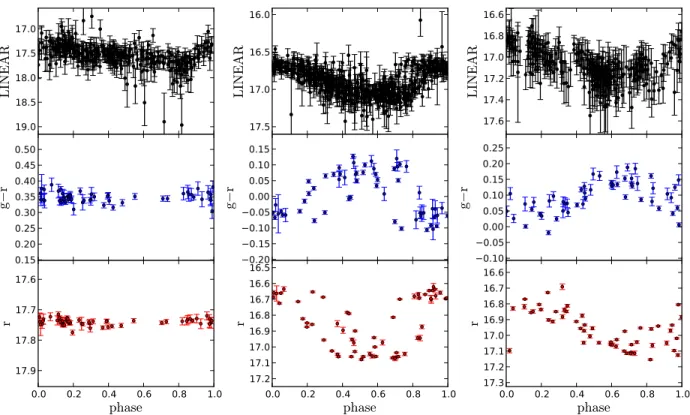
Out of 226 LINEAR objects tagged as RR Lyrae stars in the SDSS Stripe 82 by our selection algorithm, only 6 (or ∼ 3%) are not in the Ses10 Stripe 82 sample of RR Lyrae stars. One possibility is that these objects are non-RR Lyrae stars. Alternatively, some or all of them may be true RR Lyrae stars that were overlooked by Ses10 and therefore were not included in their final sample (i.e., the Ses10 sample may not be complete). To find whether any of these 6 stars are RR Lyrae stars, we phase their LINEAR and SDSS g- and r-band observations using the best-fit period determined from LINEAR data, and plot their phased light curves in Figure 2 for visual inspection.
Their phased light curves reveal that 4 out 6 objects have noisy LINEAR light curves (objects are faint and have m0 > 17 mag), and show no significant variability in SDSS
data. Noisy LINEAR light curves are the most likely reason why these spurious, non-variable objects end up in our RR Lyrae sample. The remaining two objects show significant variability in SDSS data: one is possibly a Blaˇzko or a double-mode (type-d) RR Lyrae star while the other variable object is probably not a RR Lyrae star.
The above analysis suggests that our selection algorithm produces a RR Lyrae sample where only up to ∼2% of objects are non-RR Lyrae stars. The majority of contaminants are spurious, non-variable objects with noisy LINEAR data. Since the RR Lyrae sample is mostly contaminated at the faint end, special attention needs to be given to distant halo overdensities as these are more likely to contain non-RR Lyrae stars and therefore, more likely to be spurious. This analysis also suggests that the completeness of the Ses10 sample is very high, with plausibly only one RR Lyrae star missed by Ses10 in the range r < 17 (the magnitude range probed by LINEAR).
2.5. Completeness of the LINEAR sample of RR Lyrae stars
The completeness, or the fraction of RR Lyrae stars recovered as a function of magni-tude, is another important quantity that needs to be understood before the spatial distribu-tion of RR Lyrae stars can be analyzed. To quantify completeness, we again use the Ses10 sample of RR Lyrae stars as the “ground truth” and assume the sample is complete and clean based on the analyses presented in the previous two subsections.
The completeness as a function of peak magnitude m0 is defined as the ratio
fcompleteness(m0) =Nselected(m0)/Nall(m0), (12)
where Nselected is the number of SDSS Stripe 82 RR Lyrae stars that have been tagged by
our selection algorithm and Nall is the number of all SDSS Stripe 82 RR Lyrae stars in a
magnitude bin centered on m0. The peak brightness of an SDSS Stripe 82 RR Lyrae star in
the LINEAR photometric system (m0) is calculated using its best-fit peak brightness in the
SDSS r-band light curve (r0; see Table 2 in Sesar et al. 2010b) as
m0 =r0+ 0.0574, (13)
where the 0.0574 mag offset accounts for a small magnitude zero-point shift between SDSS and LINEAR photometric systems (see Equation 6 in Sesar et al. 2011b). A comparison of synthetic and observed m0 values shows that the two are similar within 0.04 mag, as
estimated by their rms scatter.
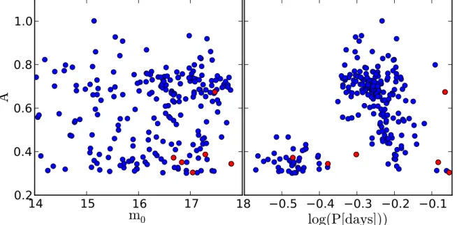
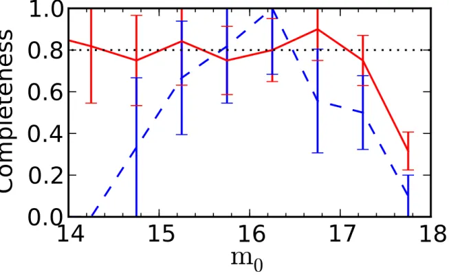
The two types of RR Lyrae stars show a different dependence of completeness on peak magnitudem0, as illustrated in Fig. 4. While the completeness of type abRR Lyrae stars is
estimated at∼80% and is seemingly independent of magnitude form0 <17.2 (corresponding
to heliocentric distances from 5 kpc to 23 kpc), the completeness of type c RR Lyrae shows a strong dependence on magnitude, with low completeness at the bright and faint ends, and a peak at m0 ∼16.2 (but note the size of Poisson error bars).
Detailed analysis has demonstrated that the amplitude cut A >0.3 mag, together with low typical amplitudes of RRc stars (A ∼ 0.3 mag, see Figure 3) are the main reasons for low completeness of RRc stars (the increase in completeness of RRc stars towardsm0 ∼16.2
is likely due to Poisson noise). We could have lowered the cut on amplitude to include more RRc stars, but that would then increase the overall contamination of the more numerous RRab sample, which we wanted to keep low per discussion in Section 2.4.
3. LINEAR catalog of RR Lyrae stars
There are 533,189 point-like (SDSS objtype=6) objects in the LINEAR database that satisfy conditions given by Equations 1–4 and 6–7. Out of this sample, we have selected 4067 typeab(hereafter RRab stars) and 834 typecRR Lyrae stars (hereafter, RRc stars) following the procedure described in Section 2. Equatorial J2000.0 right ascension and declination of selected RRab and RRc stars are listed2 in Table 1. For a catalog of RR Lyrae stars in SDSS
Stripe 82, we instead suggest the more complete and deeper Ses10 catalog be used.
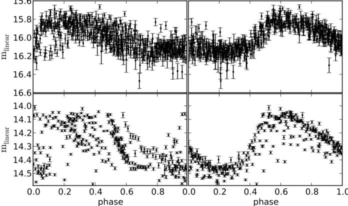
3.1. Final estimation of light curve parameters
Visual inspection of phased light curves has revealed that a non-negligible number of LINEAR RR Lyrae stars have underestimated best-fit light curve amplitudes. As shown in the top plot of Figure 5, some of these stars have two or more different maxima and are most likely undergoing light curve modulations (i.e., the Blaˇzko effect; Blaˇzko 1907; Buchler & Koll´ath 2011). Determining the true amplitude of such stars may not even be pos-sible as the Blaˇzko cycle does not always repeat regularly (Chadid et al. 2010; Kolenberg et al. 2011; S´odor et al. 2011).
In other cases (bottom plot in Figure 5), the light curve amplitude is underestimated because the best-fit template does not adequately model the observed light curve. That some light curves are not adequately modeled is expected because the light curve template set provided by Ses10 is not all-inclusive (see Figure 7 in Ses10). This inadequate modeling
does not affect the selection procedure as the quality of a template fit (ζ parameter; see Equation 5) is not used during selection. The amplitudes, which are used during selection, are underestimated only for RRab stars with light curve amplitudes greater than 0.5 mag, and such stars are already above the A > 0.3 mag selection cut (Equation 9). However, inadequate light curve modeling is a problem as amplitudes (used in Section 4) and flux-averaged magnitudes (used in Section 3.2) are derived from best-fit model light curves.
We address the issue of inadequate template fits by re-fitting LINEAR RR Lyrae light curves with new templates created from the LINEAR RR Lyrae light curve set itself, follow-ing procedure from Ses10. The new templates are constructed by interpolatfollow-ing a B-spline through phased light curves of ∼ 400 brightest, well-sampled, and visually inspected LIN-EAR RRab and RRc light curves that do not seem to be affected by Blaˇzko variations. These templates are normalized to the [0,1] range in magnitude and then fit to all LINEAR RR Lyrae light curves. The final light curve parameters are listed in Table 1.
We emphasize that the point of constructing these templates is simply to provide more accurate model light curves for LINEAR RR Lyrae stars, as these model light curves are used later in the paper. We did not attempt to prune the template set by averaging templates with similar shapes (as done by Ses10), and do not suggest that this new template set should replace the light curve template set constructed by Ses10. However, we do provide the new templates to support future work at extending RR Lyrae template light curves (templates are provided as supplementary data in the electronic edition of the journal).
Table 1 also contains 447 RRab and 336 RRc stars from the LINEAR Catalog of Variable Stars (Palaversa, L. et al., submitted to AJ). These RR Lyrae stars were missed by our selection algorithm and are included for completeness. However, they are not used in the analysis below and their exclusion does not significantly change our results.
3.2. Heliocentric Distances
The heliocentric distances of RR Lyrae stars, D, are calculated as
D= 10(hmi−MRR)/5+1/1000 kpc, (14)
where hmi is the flux-averaged LINEAR magnitude and MRR is the absolute magnitude
of RR Lyrae stars in the LINEAR bandpass. The flux-averaged magnitude is calculated by first converting the best-fit model light curve, A T(φ) +m0, into flux units (A, T(φ),
and m0 are the best-fit amplitude, template, and peak brightness, respectively). This
curve is then integrated and the result is converted back to magnitudes. The flux-averaged magnitudes, listed in Table 1, are also corrected for interstellar medium (ISM) extinction
hmi=hminot corrected−rExt, where rExt = 2.751E(B−V) is the extinction in SDSSr band,
and E(B−V) color excess is provided by the Schlegel et al. (1998) dust map.
For RRab stars, we adopt MRR = 0.6±0.1 as their absolute magnitude. The absolute
magnitude was calculated using the Chaboyer (1999) MV −[Fe/H] relation
MV = (0.23±0.04)[Fe/H] + (0.93±0.12), (15)
where we assume that the metallicity of RRab stars is equal to the median metallicity of halo stars ([Fe/H] =−1.5; Ivezi´c et al. 2008). We also assume that the absolute magnitudes of RRab stars in the LINEAR and Johnson V bandpasses are approximately equal. The estimate of the uncertainty in absolute magnitude is detailed in the next paragraph. For RRc stars, we simply adopt MRR = 0.5±0.1 mag (Kollmeier et al. 2012).
There are three significant sources of uncertainty in the adopted absolute magnitude. First, the MRR ≈ MV approximation is uncertain at ∼ 0.04 mag level (in rms). This
uncertainty was estimated by comparing LINEAR and V-band flux-averaged magnitudes of RR Lyrae stars which have multi-epoch data from SDSS Stripe 82. The V-band flux-averaged magnitudes were calculated from synthetic V-band light curves following Section 4.1 by Ses10. Second, the metallicity dispersion in the Galactic halo is about σ[F e/H] = 0.3
dex (Ivezi´c et al. 2008), and introduces about σM[F e/HV ] = 0.07 mag of uncertainty due to the assumption that all RRab stars have the same metallicity. And third, there is about σev
MV = 0.08 mag of uncertainty due to RR Lyrae evolution off the zero-age horizontal branch
(Vivas & Zinn 2006). By adding all these uncertainties in quadrature, the final uncertainty in the absolute magnitude of RRab stars is about 0.1 mag, implying∼5% fractional uncertainty in distance.
In the rest of this work we only use RRab stars. TypecRR RRLyrae stars are not used due to their much lower completeness (see Section 2.5 and Figure 4).
4. Period-Amplitude Distribution
As suggested by Catelan (2009), the period-amplitude distribution of RR Lyrae stars may hold clues about the formation history of the Galactic halo. Catelan points to a sharp division (a dichotomy first noted by Oosterhoff 1939) in the average period of RRab stars in Galactic globular clusters, hPabi; there are Oosterhoff type I (Oo I) globular clusters with hPabi ∼ 0.55 days, Oosterhoff type II (Oo II) globular clusters with hPabi ∼ 0.65 days, and
very few clusters with hPabi in between. On the other hand, the dwarf spheroidal satellite
0.62; see his Figure 5). Catelan (2009) further argues that, if the Oosterhoff dichotomy is present in the period-amplitude distribution of fieldhalo RRab stars, then the Galactic halo could not have been entirely assembled by the accretion of dwarf galaxies resembling the present-day Milky Way satellites. In light of these conclusions, it is interesting to examine the period-amplitude distribution of LINEAR RRab stars and see whether the Oosterhoff dichotomy is also present among the Galactic halo field RRab stars.
A period-amplitude diagram for RRab stars listed in Table 1 is shown in Figure 6. A locus of stars is clearly visible in this diagram. We trace this locus by binning logP values in narrow amplitude bins, and then calculate the median logP value in each bin. To model the locus in the logP vs. amplitude diagram, we fit a quadratic function to medians and obtain
logP =−0.16625223−0.07021281A−0.06272357A2 (16) as the best fit. The solid line in Figure 6 (top) is very similar to the period-amplitude line of RRab stars in the globular cluster M3 (see Figure 3 by Cacciari et al. 2005). Since M3 is the prototype Oo I globular cluster, we label the main locus as the Oo I locus.
The contours in Figure 6 (top) seem to indicate a presence of a second locus of RRab stars to the right of the Oo I locus. To examine this in more detail, we calculate the period shift, ∆ logP, of RRab stars from the Oo I locus and at a fixed amplitude. The distribution of ∆ logP, shown in Figure 6 (bottom), is centered on zero (the position of the Oo I locus), and has a long-period tail. Even though we do not see the clearly displaced secondary peak that is usually associated with an Oo II component (see Figure 21 by Miceli et al. 2008), hereafter we will refer to stars in the long-period tail as Oo II RRab stars.
To separate the two Oosterhoff types, we model the Oo I peak with a Gaussian and find that this Gaussian roughly ends at ∆ logP = 0.05. RRab stars with ∆ logP <0.05 (where period is measured in days) are tagged as Oo I RRab stars, and those with ∆ logP ≥ 0.05 are tagged as Oo II RRab stars. We find the ratio of Oo II to Oo I RRab stars in the halo to be 1:4 (0.25). A similar ratio was found by Miceli et al. (2008) and Drake et al. (2013) (26% and 24%, respectively).
5. Number Density Distribution
In this Section, we introduce a method for estimating the number density distribution of RR Lyrae stars that is less sensitive to the presence of halo substructures (streams and overdensities). The method is first illustrated and tested on a mock sample of RR Lyrae stars drawn from a known number density distribution. The purpose of this test is to estimate
the precision of the method in recovering the input model. At the end of this section, the method is applied to the observed spatial distribution of LINEAR RRab stars.
We begin by drawing ten mock samples of RRab stars from the following number density distribution: ρmodel(X, Y, Z) =ρRR⊙ R⊙ r n (17) r =pX2+Y2+ (Z/q)2, (18) where ρRR
⊙ = 4.5 kpc−3 is the number density of RRab stars at the position of the Sun
(R⊙ = 8 kpc or (X⊙, Y⊙, Z⊙) = (8, 0, 0) kpc), q = 0.71 is the ratio of major axes in the
Z and X directions indicating that the halo is oblate (flattened in the Z direction), and n = 2.62 is the power-law index. The above model was motivated by Juri´c et al. (2008), who used a similar model to describe the number density distribution of halo main-sequence stars selected from SDSS. TheX,Y, and Z are coordinates in the Cartesian galactocentric coordinate system
X =R⊙−Dcoslcosb, (19)
Y =−Dsinlcosb, (20)
Z =Dsinb, (21)
where l and b are Galactic longitude and latitude in degrees, respectively.
The number density model defined by Equation 17 is assumed to be a fair representation of the actual number density distribution of halo RRab stars. The parameters used in the above model were selected based on previous studies of the Galactic halo. Sesar et al. (2011a) have found that a two parameter, single power-law ellipsoid model (i.e., Equation 17) with q = 0.71±0.01 and n = 2.62±0.04 provides a good description of the number density distribution of halo main-sequence stars within 30 kpc of the Galactic center. Since halo main-sequence stars are progenitors of RR Lyrae stars, it is reasonable to assume that shapes of their number density distributions are similar as well. The number density of RRab stars at the position of the Sun (ρRR
⊙ ) has been estimated by several studies so far, yielding values
ranging from 4 to 5 kpc−3 (Preston et al. 1991; Suntzeff et al. 1991; Vivas & Zinn 2006).
The mock samples were generated using Galfast3 code, which provides the position, magnitude and distance modulus for each star. To simulate the uncertainty in heliocentric distance characteristic of the LINEAR sample of RRab stars, we add Gaussian noise to
3
true distances provided by Galfast (D0) using a 0.1 mag wide Gaussian centered at zero,
D=D010N(0,0.1)/5.
The presence of halo substructure is simulated by adding a clump of about 620 stars to each mock sample (i.e., about 17% of stars are in the substructure) and by distributing them in a uniform sphere 2 kpc wide and centered on (X, Y, Z)=(8, 0, 10) kpc (i.e., roughly in the center of the probed volume of the Galactic halo). Finally, each sample is trimmed down to match the spatial coverage of the LINEAR sample of RRab stars using the following cuts:
b >30◦, (22) δJ2000 <−1.2αJ2000+ 362◦, (23) −4◦ < δ J2000 <72◦, (24) δJ2000 <0.73αJ2000−26.6◦, (25) δJ2000 >1.38αJ2000−338.52◦, (26) 5 kpc< D < 23 kpc, (27) Z >3 kpc, (28)
whereαJ2000andδJ2000are equatorial right ascension and declination in degrees, respectively.
The penultimate cut limits the samples to distances where the LINEAR sample of RRab stars is 80% complete, and with the last cut we minimize possible contamination by thick disk stars. Note that mock samplesdo notsuffer from any incompleteness or contamination. The reason we are applying the above cuts to mock samples is because the same cuts will later be applied to the observed sample of LINEAR RRab stars, which does suffer from incompleteness at greater distances and may have some contamination from thick disk RRab stars.
The spatial distribution of stars in each mock sample traces the underlying number density distribution. To compute the number density of stars at someXY Z position in the Galactic halo, we use a Bayesian estimator developed by Ivezi´c et al. (2005, also see Chapter 6.1 of Ivezi´c et al. 2013): ρ(X, Y, Z) = 3(m+ 1) 4π 1 PNnn k=1d3k = 111 4π 1 P8 k=1[(X−Xk)2+ (Y −Yk)2+ (Z −Zk)2] 3/2, (29) whereNnn = 8 is the number of nearest neighbors to which the distancedin a 3-dimensional
space is calculated, m =Nnn(Nnn+ 1)/2 = 36, and (Xk, Yk, Zk) is the position of the k-th
nearest neighbor in Cartesian galactocentric coordinates. The volume of the Galactic halo probed by LINEAR RR Lyrae stars is binned in 0.1×0.1×0.1 kpc3 bins, and the number
are removed to minimize edge effects. In total, the number density is calculated for about 6 million bins.
Having calculated number densities on a grid, we can now fit Equation 17 to computed number densities in order to find the best-fit n, q, and ρRR
⊙ . Standard χ2 minimization
algorithms (e.g., the Levenberg-Marquardt algorithm; Press et al. 1992) are susceptible to outliers in data, such as unidentified overdensities, and produce biased results unless outliers are removed. Since we would rather avoid ad hoc removal of suspected outliers, we use a fitting method that is instead robust to the presence of outliers.
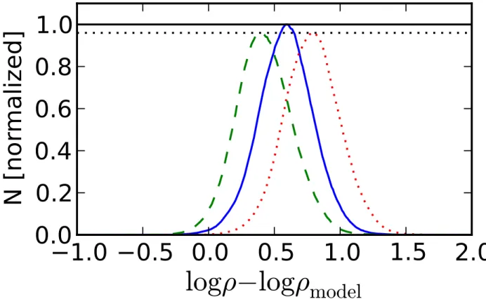
The basic principle of our fitting method is illustrated in Figure 7. When the correct model is used, the height of the distribution of ∆ logρ = logρ−logρmodel values is greater
than when an incorrect model is used. The influence of substructures is attenuated because overdense regions have highly positive values of ∆ logρ (i.e., they are in the wings of the distribution), and thus have little effect on the height of the ∆ logρ distribution. Note that in this method, ρRR
⊙ is not a free parameter; ρRR⊙ is simply estimated as the mode of the
∆ logρ distribution raised to the power of 10.
Due to sparseness of the sample (i.e., Poisson noise), logρ values will have a certain level of uncertainty. This uncertainty, or the average random error in logρ, can be estimated from the rms scatter of ∆ logρ values for the correct model. We find this value to be ∼0.2 dex. While the average random error can be decreased by increasing the number of nearest neighbors used when computing the density, the downside is an increase in edge effects if the sample is too sparse.
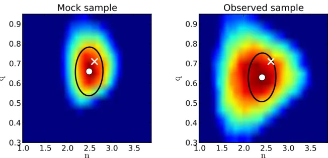
The best-fit values ofnandq parameters are determined by measuring the height of the ∆ logρ distribution on a fixed n vs. q grid. A “height” map for one of the mock RR Lyrae samples generated using Galfast is shown in Figure 8 (left). Due to sparseness of the sample (Poisson noise), the best-fit values ofn andq parameters will not necessarily be exactly the same as input n and q values. To estimate the statistical uncertainty in best-fit n and q parameters due to Poisson noise, we do the fitting on all ten mock samples and analyze the distribution of best-fit parameters. We find thatρRR
⊙ = 4.4±0.6 kpc−3, q= 0.73±0.05, and
n = 2.63±0.13, where the errors represent the rms scatter (recall that the true values are ρRR
⊙ = 4.5 kpc−3, q= 0.71, andn = 2.62).
Finally, we apply the above procedure to the observed sample of LINEAR RRab stars. We find that the distribution of RRab stars in the Galactic halo between 5 and 23 kpc can be modeled as an oblate, single power-law ellipsoid (Equation 17) with the oblateness q= 0.63±0.05 and power-law index n= 2.42±0.13. The uncertainties on these parameters were adopted from the analysis of mock samples described above. The best-fit values are
consistent within the 95% confidence limit with values determined by Sesar et al. (2011a) for the number density distribution of halo main-sequence stars (q = 0.71±0.01,n= 2.62±0.04). The number density of RRab stars at the position of the Sun is ρRR
⊙ = 4.5±0.6 kpc−3, or
ρRR
⊙ = 5.6±0.8 kpc−3 once the measured number density is increased by 20% to account
for completeness of the LINEAR sample of RRab stars (estimated at 80% in Section 2.5). Adoptingq = 0.71 and n= 2.62 from Sesar et al. (2011a), we obtain ρRR
⊙ = 4.9±0.6 kpc−3,
or ρRR
⊙ = 5.9±0.8 kpc−3 once the measured number density is increased to account for
completeness.
Applying the above procedure to Oo I RRab stars we obtain q = 0.59±0.05, n = 2.4±0.09, andρRR
⊙ = 4.0±0.7 kpc−3(ρRR⊙ = 5.0±0.9 kpc−3when corrected for completeness).
For the Oo II subsample, we obtain q = 0.56±0.07, n = 3.1±0.2, and ρRR
⊙ = 2.1±1.0
kpc−3 (ρRR
⊙ = 2.6±1.3 kpc−3 when corrected for completeness). The uncertainties on these
parameters were adopted from the analysis of mock Oo I and Oo II RRab samples. The “height” maps for the Oo I and Oo II RRab subsamples are shown in Figure 9. These power-law indices are consistent with indices obtained by Miceli et al. (2008) for LONEOS-I Oo I and Oo II RRab subsamples (see their Table 3).
5.1. Rejection of a Simple Power-Law Model
The best-fit number density model of the full RRab sample (n = 2.4, q = 0.63) is consistent with previous models for the number density profiles within 30 kpc from the Galactic center of i) RR Lyrae stars (n= 2.4 assumingq = 1.0, Watkins et al. 2009;n = 2.3 assuming q = 0.64, Sesar et al. 2010b), ii) metal-poor main-sequence stars (n = 2.6 and q = 0.7, Sesar et al. 2011a), and iii) blue horizontal branch stars (n = 2.4 and q = 0.6, Deason et al. 2011). However, a closer inspection of ∆ logρ residuals in the R vs. Z map (top left panel in Figure 10), indicates that the best-fit single power-law model overestimates the observed number density of RRab stars for r < 16 kpc. As shown in Figure 11 (thick solid line), the model at r∼5 kpc predicts about 3 times more stars than observed.
A possible explanation for this discrepancy could be the incompleteness of the RRab sample at distances closer than 16 kpc. However, this is unlikely as Figure 4 shows the completeness of RRab stars to be about ∼ 80% within 20 kpc. Adding RR Lyrae stars from the LINEAR Catalog of Variable Stars (see the end of Section 3.1) does not alleviate this discrepancy. Another possible explanation is an inadequate model for number density variation with position.
power-law index. The former is not supported by data: when two subsamples selected by Rgc <12 kpc andRgc>12 kpc are fit separately, the best-fitqis essentially unchanged. This
invariance of oblateness with distance is consistent with several recent studies (Miceli et al. 2008; Sesar et al. 2011a; Deason et al. 2011).
A double power-law model is one possible extension of the single power-law model used above. When a double power-law model with oblateness parameter q = 0.65±0.03, inner power-law index ninner = 1.0±0.3, outer power-law index of nouter= 2.7±0.3, and a break
radius at rbr =
p
X2+Y2+ (Z/q)2 = 16±1 kpc is fit to data, the residuals improve, but
the model now underestimates the observed number densities within r.10 (see Figures 10 and 11). Again, the errors on best-fit parameters are statistical uncertainties adopted from the analysis of mock RRab samples, as done in the previous Section. The remaining residuals within r . 10 may be (again) due to an inadequate model or they may be due to an overdensity (a diffuse overdensity has been reported in this region, see Figure 13). A power-law with an index of n = 2.5 can model the residuals within r . 10 fairly well, but that would mean that the number density distribution of RR Lyrae stars in the halo has a much more complicated shape than ever reported (three power-laws).
Another possible explanation for the peculiar shape of the observed number density distribution is that the halo does not have a smooth distribution of RR Lyrae stars, with an occasional overdensity imprinted on top of it, but that the distribution is more clumpy. To verify this hypothesis, we generated a mock sample consisting of 400 uniform spheres with a radius of 2 kpc, with each sphere containing 7 stars. The residuals obtained after fitting a single power-law model to the number density distribution of this clumpy mock sample are shown in Figure 10 (bottom right panel) and Figure 11 (dotted line). As evident from Figure 11, the residuals for the clumpy mock sample and the observed sample exhibit similar trends with logr when fitted with a single power-law. The agreement is qualitative enough to suggest that the shape of the observed number density distribution of RRab stars could be due to a purely clumpy halo.
We have used a broken power law to separately model the number densities of the Oo I and Oo II samples. For the former, the best-fit parameters are the same as for the full sample (recall that Oo I stars account for 75% of the full sample). The best parameters for the Oo II sample are q = 0.60, ninner = 1.6, nouter = 3.4, rbr = 18 kpc, and ρRR⊙ = 0.6±0.5 kpc−3.
Therefore, for both single and broken power-law models, the number density distribution for the Oo II subsample is steeper than for the Oo I subsample.
6. Halo Substructures
In the previous Section, we used the spatial distribution of LINEAR RRab stars to estimate the best-fit smooth model for their number density distribution. In this Section, we use a group-finding algorithm EnLink (Sharma & Johnston 2009) to identify significant clusters of RR Lyrae stars (halo substructures). The search for halo substructures is done using LINEAR RRab stars that pass Equations 22–28. The sample of RRab stars is not split by Oosterhoff type so that groups that are “Oosterhoff intermediate”, i.e., groups that may be associated with remnants of dSph galaxies, can be detected as well.
The algorithm EnLink has two free parameters which need to be supplied by the user. The first parameter is the number of nearest neighbors employed for density estimation,kden.
Sharma & Johnston (2009) find thatkden= 30 is appropriate for most clustering tasks, and
we adopt their value. The second parameter is the significance threshold Sth. Clusters of
points that have significance S below threshold Sth are denied the status of a group and are
merged with the background.
Sharma & Johnston (2009) define the statistical significance S for a group as a ratio of signal associated with a group to the noise in the measurement of this signal. The contrast, ln(ρmax)−ln(ρmin) between the peak density of a group (ρmax) and valley (ρmin) where it
overlaps with another group can be thought of as the signal, and the noise in this signal is given by the varianceσlnρ associated with the density estimator (σlnρ= 0.22 for kden = 30).
Combining the definitions of signal and noise then leads to S = (ln(ρmax)−ln(ρmin))/σlnρ.
Selecting the value of Sth is not trivial. For values of Sth that are too low, EnLink
may detect spurious groups (i.e., groups produced by Poisson noise). On the other hand, a threshold that is too high might miss real halo substructures.
To find the optimal choice ofSthfor our sample of LINEAR RRab stars, we run EnLink
on ten mock samples of RRab stars drawn from a number density distribution defined by Equation 17, where n = 2.42, q = 0.63, and ρRR
⊙ = 4.5 kpc−3 (the best-fit single power-law
model; see Section 5). While this model may not be the best description of the number density distribution of RRab stars in the halo (i.e., it overestimates the number of RRab stars, see Section 5.1), it is still useful. Mock samples drawn from this model will have a higher chance of producing spurious groups (simply because they contain more stars), and thus the number of spurious groups detected in such samples can serve as an upper limit on the number of spurious groups that one may expect to find in the observed sample.
To make mock samples similar to our sample of LINEAR RRab stars, we add noise to heliocentric distances in mock samples and then trim down samples using Equations 22 to 28. The EnLink algorithm is applied to each mock sample and the number of detected
groups and the fraction of stars in groups as a function of Sth is recorded. The results are
shown in Figure 14.
When the significance threshold Sth is low (Sth < 0.7), EnLink detects several groups
in mock samples. These groups are spurious, have low significance, and they arise due to Poisson noise. As the threshold Sth increases, the number of groups in mock samples
decreases (i.e., random fluctuations are not likely to create highly significant groups). The number of groups detected in the observed sample also decreases with increasing Sth, but at
a different rate. ForSth = 1.4, EnLink detects seven groups in the observed sample and on
average one (spurious) group in mock samples. By increasing the significance threshold to 2.5, we could eliminate the possibility of detecting a spurious group in the observed sample, but the number of detected groups would drop to two. We selectSth = 1.4 as the significance
threshold; this choice results in one expected spurious group.
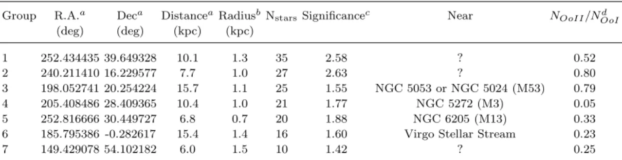
The positions of detected groups, number of stars in a group, and significance of a group are listed in Table 2. The spatial distribution of RRab stars associated with these groups is shown in Figures 15 and 16. The stars associated with these groups are also appropriately labeled in Table 1 (see column “Group ID”). On average, the groups have radii of ∼1 kpc, where the radius is the median distance of stars in a group from the peak in number density for that group.
6.1. Detected Groups
Of the seven groups, three groups (groups 3, 4, 5) are near globular clusters (M53 or NGC 5053, M3, and M13), and one group (group 6) is located in the Virgo constellation where several halo substructures have already been reported (Vivas et al. 2001; Newberg et al. 2002; Duffau et al. 2006; Juri´c et al. 2008). The groups 3 and 4 are not isotropic and seem to have a stream-like morphology (Figure 16). For example, group 4, which is located near the globular cluster M3, extends ∼4 kpc roughly parallel to the Galactic plane, and makes
∼ 45◦ angle with the Sun–Galactic Center line. Group 3, which is located near globular clusters M53 and NGC 5053, on the other hand, extends more towards the Galactic plane. Previous studies have detected tidal streams around NGC 5053 and M53 (Lauchner et al. 2006; Chun et al. 2010), and no streams have been detected around M3 (Grillmair & Johnson 2006).
The seemingly non-isotropic distribution of RRab stars in group 5, which is near globular cluster M13, is likely due to limited spatial coverage (the group is close to the edge of the probed volume). However, even though this group is near globular cluster M13, its
relationship with the cluster is quite tenuous since M13 is known to have a very small number of RR Lyrae stars (Clement et al. 2001).
Groups 1, 2, and 7 do not seem to be near any known halo substructures (e.g., the Sagittarius tidal streams), dSph galaxies or globular clusters. Globular clusters M92 and M13 are the closest clusters to group 1, but they are still off by ∼3 kpc in heliocentric distance. This offset is well outside the uncertainty in distance, especially since the metallicities of clusters are known and can be used to calculate the absolute magnitudes of RRab stars potentially originating from clusters (using Equation 15). Group 7 contains only ten RRab stars and has borderline significance (S = 1.42). Thus, this group is the one most likely to be spurious.
The ratio of Oosterhoff type II (Oo II) to Oosterhoff type I (Oo I) RRab stars in a group may provide additional clues on the nature of detected groups. As shown in Section 4, this ratio is 1:4 for the halo. For group 4, this ratio is close to zero (0.05; see Table 2), indicating that the group 4 is dominated by Oo I RRab stars. This result is interesting because M3 is classified as an Oo I-type globular cluster (Catelan 2009) and is located within group 4 (see bottom panel in Figure 17). Thus, the fact that the group 4 and the globular cluster M3 have the same Oosterhoff type may indicate their common origin.
Group 3 is near globular clusters NGC 5053 and M53, both of which are classified as Oo II-type globular clusters (Catelan 2009). Again, we find many more Oo II RRab stars from this group near the centers of globular clusters NGC 5053 and M53 (bottom panel in Figure 18), and the group as a whole has a higher ratio of Oo II to Oo I RRab stars (0.79). The reason we are not detecting more Oo II RRab stars and the reason this ratio is not much higher for this particular group is due to the incompleteness of the LINEAR RRab sample in crowded regions (e.g., near centers of globular clusters).
Group 3 may actually consist of two groups of stars that were joined by EnLink into a single group. Looking at group 3 in Figure 16, we can discern a “stream” of points that is parallel to the Galactic plane, and spans ∼ 4 kpc at ∼ 13.5 kpc above the Galactic plane. The ratio of Oosterhoff II to I types in this subgroup is 1:2, or higher than in the halo. Based on the morphology of this subgroup and its distance from the globular clusters M53 and NGC 5053 (∼2−3 kpc), this subgroup may be a separate halo substructure that EnLink joined with the NGC 5053/M53 group of RRab stars.
It is worth mentioning that although M53 and NGC 5053 are relatively close to each other in space, they have radial velocities that differ by more than 100 km s−1 (Harris 1996
catalog, 2010 edition). Followup spectroscopic studies should take advantage of this fact when associating group 3 and its parts with either of these globular clusters.
In principle, the proper motions of clusters could be used to identify RR Lyrae stars that were tidally stripped, as such stars would follow the motion of the clusters. In the case of M53 and NGC 5053, there are a few RR Lyrae stars nearR.A. ∼196◦ andDec∼19◦ (see the bottom panel of Figure 18) that roughly align with the proper motion vector of M53 and with the tidal stream reported by Lauchner et al. (2006). These stars may have been tidally stripped and may be trailing M53 or NGC 5053. However, since the proper motion of M53 is quite uncertain (µαcosδ= 0.5±1.0 mas yr−1,µδ =−0.1±1.0 mas yr−1; Odenkirchen et al.
1997), and since the proper motion of NGC 5053 has not yet been reported, it is difficult to judge whether this is truly the case. In the case of M3, the RR Lyrae stars in group 4 spread in the east-west direction (see the bottom panel of Figure 17), or almost perpendicular to the proper motion vector of M3 (µαcosδ = −0.06±0.3 mas yr−1, µδ = −0.26±0.3 mas
yr−1; Wu et al. 2002). While this observation could be used as an argument against the
claim that the extended parts of group 4 share a common origin with the globular cluster M3, we do point out that the measured proper motion of M3 is still quite uncertain.
Group 6, which is located in the Virgo constellation where several halo substructures have been reported so far, has the ratio of Oosterhoff types that is consistent to the one found for the halo (0.23 vs. 0.25).
Groups 1 and 2 have Oosterhoff types ratios that are higher by a factor of 2 and 3, respectively, relative to the halo. Assuming that the number density distributions of Oo I and Oo II RRab stars in the halo are the same, the probabilities of drawing groups 1 and 2 are 0.07 and 0.01. For comparison, the probability of drawing group 6 (in the Virgo constellation) is 0.21, 0.28 for group 7, and 0.23 for the subgroup of group 3.
7. Discussion and Conclusions
This paper is the second one in a series based on light curve data collected by the asteroid LINEAR survey. In the first paper, Sesar et al. (2011b) described the LINEAR survey and photometric recalibration based on SDSS stars acting as a dense grid of standard stars. Here, we searched the LINEAR dataset for variable RR Lyrae stars and used them to study the Galactic halo structure and substructures.
While this paper was in preparation, a study of RR Lyrae stars selected from the Catalina Surveys Data Release 1 (CSDR1) was announced (Drake et al. 2013). The two works are largely complementary in terms of science; while Drake et al. analyzed radial velocity and metallicity distributions of CSDR1 RR Lyrae stars with spectroscopic mea-surements from SDSS and focused on the Sagittarius stream, we searched for new halo
substructures and studied the number density distribution of RR Lyrae stars as a whole and by Oosterhoff type.
In total, we have selected 4067 type ab and 834 type c RR Lyrae stars from the recali-brated LINEAR dataset. These stars probe∼8000 deg2 of sky to 30 kpc from the Sun. The
LINEAR sample of RR Lyrae stars has low contamination (∼2%) and is ∼80% complete to 23 kpc from the Sun. To facilitate follow-up studies, the coordinates and light curve proper-ties (amplitude, period, etc.) of stars in this sample are made publicly available, as well as their Oosterhoff classification and whether they are associated with a halo substructure.
We also provide light curve templates that were derived from phased light curves of
∼400 bright LINEAR RRab and RRc stars. Even though we used these templates to obtain more accurate model light curves of LINEAR RR Lyrae stars, we emphasize that we did not attempt to prune the template set by averaging templates with similar shapes (as done by Ses10), and do not suggest that this new template set should replace the light curve template set constructed by Ses10. However, we do provide the new templates to support future work at extending RR Lyrae template light curves (templates are provided as supplementary data in the electronic edition of the journal).
We find evidence for the Oosterhoff dichotomy among field RR Lyrae stars. While we do not see the clearly displaced secondary peak in the ∆ logP diagram (bottom panel in Figure 6) that is usually associated with an Oo II component (e.g., see Figure 21 by Miceli et al. 2008), we do detect a long tail that contains RRab stars with periods consistent with Oosterhoff type II RRab stars. The ratio of the number of stars in the Oosterhoff II and I subsamples is 1:4. A similar ratio was found by Miceli et al. (2008) and Drake et al. (2013) (0.26 and 0.24, respectively).
The lack of a clear gap in the ∆ logP distribution between the two components may be a combination of two factors. First, this region in the ∆ logP diagram may contain “Oosterhoff intermediate” RR Lyrae stars. As these stars are presumed to come from dwarf galaxies similar to present-day Milky Way dSph satellite galaxies (Catelan 2009), the lack of a gap may be evidence that some fraction of stars were accreted from such systems. Second, the gap may be filled by short-period Oosterhoff type II RR Lyrae stars that are undergoing Blaˇzko variations. If they are not observed at the maximum of their Blaˇzko cycle when their light curve amplitude is the greatest, or if their maximum light curve amplitude is not recognized in the folded data, these stars will scatter towards lower amplitudes at the same period and will fill in the gap between the two Oosterhoff components.
The wide coverage and depth of the LINEAR RRab sample allowed us to study the number density distribution of halo RRab stars to a much greater extent than it was possible
in previous studies. We find it possible to describe the number density of RRab stars by an oblate 1/rnellipsoid, with the axis ratioq = 0.63 and the power-law index ofn = 2.42. These
values are consistent with previous models for the number density of various tracers within 30 kpc from the Galactic center (Watkins et al. 2009; Sesar et al. 2010b, 2011a; Deason et al. 2011).
However, as discussed in Section 5.1 and as illustrated in Figure 12, the single power-law model overestimates the number density of RRab stars within r ∼16 kpc. Analysis done in Section 2.5 excludes incompleteness as a likely explanation for this discrepancy. Potential problems with the fitting method are also unlikely, as we have repeatedly tested our fitting method on several mock samples drawn from known number density distributions, and have quantified its precision in recovering input parameters in the presence of realistic distance errors and halo substructures. The discrepancy between the best-fit single power-law model and the observed number density can be decreased by using a broken (or double) power-law model, where the power-power-law index changes from ninner = 1.0 to nouter = 2.7 at the
break radius of rbr ∼ 16 kpc, with the best-fit oblateness parameter set at q = 0.65. The
variation in the power-law index is not due to the smaller Oosterhoff II component, because this subsample also shows independent evidence for a variable power-law. Alternatively, as simulations with mock samples have suggested, the observed variable power-law slope may not due to a change in the smooth distribution of stars, but may be evidence of a clumpy distribution of RR Lyrae stars within r∼16 kpc.
Possible independent evidence that may support the density profile observed in Figure 12 may be found in a recent kinematic study by Kafle et al. (2012). Kafle et al. used 4667 blue horizontal branch (BHB) stars selected from the SDSS/SEGUE survey to determine key dynamical properties of the Galactic halo, such as the profile of velocity anisotropy β
β = 1−σ 2 θ +σ2φ 2σ2 r , (30)
where σr, σθ, and σφ are the velocity dispersions in spherical coordinates. They find that
“from a starting value of β ≈ 0.5 in the inner parts (9 < r/kpc < 12), the profile falls sharply in the range r ≈ 13−18 kpc, with a minimum value of β = −1.2 at r = 17 kpc, rising sharply at larger radius”. The metal-rich and metal-poor population of BHB stars analyzed by Kafle et al. (2013) were also found to exhibit similar behaviour inβ. The range of distances where theβ sharply falls is the same range where we find that a shallower power-law with an index of 1.0 provides as better fit to observed number densities of RRab stars. This suggests that the two effects may be related to each other and may have a common cause (e.g., presence of a diffuse substructure).
sample of RRab stars and detected seven candidate halo groups, one of which may be spurious (based on a comparison with mock samples). Three of these groups are near globular clusters (groups 3, 4, and 5), and one (group 6) is near a known halo substructure (Virgo Stellar Stream; Vivas et al. 2001; Duffau et al. 2006). The extended morphology and the position (outside the tidal radius) of some of the groups near globular clusters is suggestive of tidal streams possibly originating from globular clusters. The remaining three groups do not seem to be near any known halo substructures or globular clusters. Out of these, groups 1 and 2 have a higher ratio of Oosterhoff type II to Oosterhoff type I RRab stars than what is found in the halo.
While we have done our best to quantify the significance of detected halo groups, we emphasize that these groups are just candidates whose authenticity still needs to be verified. This verification can be done by analyzing metallicities and velocities of RR Lyrae stars obtained from a spectroscopic followup (e.g., Sesar et al. 2010a, 2012). If a spatial group is real, then its stars should also cluster in the velocity and metallicity space. Such followup studies are highly encouraged and should provide more conclusive evidence on the nature of detected groups.
In this work, we used the sample of LINEAR RR Lyrae stars to study the halo structure and substructures, but its usefulness goes beyond these simple applications. For example, light curves of LINEAR RRab stars are well sampled and should allow a robust decomposition into a Fourier series. In turn, the Fourier components can be used to estimate the metallicity of RRab stars via the Jurcsik & Kovacs (1996) method. These metallicities can then be used to study the metallicity distribution of RR Lyrae stars in the halo. Searches for halo substructures will also benefit from having metallicities as these represent an additional dimension for clustering algorithms such as EnLink. As RRab stars in this sample are brighter than 17 mag, they will be observed by the upcoming surveys such as the LAMOST Experiment for Galactic Understanding and Exploration (LEGUE; Deng et al. 2012) and GAIA (Perryman 2002). These surveys will provide metallicity, proper motion, and parallax measurements for RR Lyrae stars up to 30 kpc from the Sun and will enable unprecedented studies of the structure, formation and the evolution of the Galactic halo.
B.S. thanks NSF grant AST-0908139 to Judith G. Cohen for partial support. ˇZ.I. acknowledges support by NSF grants AST-0707901 and AST-1008784 to the University of Washington, by NSF grant AST-0551161 to LSST for design and development activity, and by the Croatian National Science Foundation grant O-1548-2009. A.C.B. acknowledges support from NASA ADP grant NNX09AC77G. The LINEAR program is funded by the National Aeronautics and Space Administration at MIT Lincoln Laboratory under Air Force Contract FA8721-05-C-0002. Opinions, interpretations, conclusions and recommendations
are those of the authors and are not necessarily endorsed by the United States Government.
REFERENCES
Blaˇzko, S. 1907, Astronomische Nachrichten, 175, 325 Buchler, J. R., & Koll´ath, Z. 2011, ApJ, 731, 24
Bullock, J. S., Kravtsov, A. V., & Weinberg, D. H. 2001, ApJ, 548, 33 Cacciari, C., Corwin, T. M., & Carney, B. W. 2005, AJ, 129, 267 Catelan, M. 2009, Ap&SS, 320, 261
Chaboyer, B. 1999, Post-Hipparcos Cosmic Candles, 237, 111 Chadid, M., Benk˝o, J. M., Szab´o, R., et al. 2010, A&A, 510, A39 Chun, S.-H., Kim, J.-W., Sohn, S. T., et al. 2010, AJ, 139, 606 Clement, C. M., Muzzin, A., Dufton, Q., et al. 2001, AJ, 122, 2587 De Lee, N. 2008, PhD thesis, Michigan State University
Deason, A. J., Belokurov, V., & Evans, N. W. 2011, MNRAS, 416, 2903
Deason, A. J., Belokurov, V., Evans, N. W., & An, J. 2012, MNRAS, 424, L44
Deng, L.-C., Newberg, H. J., Liu, C., et al. 2012, Research in Astronomy and Astrophysics, 12, 735
Drake, A. J., Catelan, M., Djorgovski, S. G., et al. 2013, ApJ, 763, 32 Duffau, S., Zinn, R., Vivas, A. K., et al. 2006, ApJ, 636, L97
Freeman, K., & Bland-Hawthorn, J. 2002, ARA&A, 40, 487
Friedman, J. H. 1984, A variable span scatterplot smoother, Tech. rep., Laboratory for Computational Statistics, Stanford University, technical Report No. 5
Grillmair, C. J., & Johnson, R. 2006, ApJ, 639, L17
Harding, P., Morrison, H. L., Olszewski, E. W., et al. 2001, AJ, 122, 1397 Harris, W. E. 1996, AJ, 112, 1487
Helmi, A. 2008, A&A Rev., 15, 145
Helmi, A., & White, S. D. M. 1999, MNRAS, 307, 495 Ivezi´c, ˇZ., Beers, T. C., & Juri´c, M. 2012, ARA&A, 50, 251
Ivezi´c, ˇZ., Connoly, A., VanderPlas, J., & Gray, A. 2013, Statistics, Data Mining, and Machine Learning in Astronomy: A Practical Guide for the Analysis of Survey Data, Princeton (Princeton University Press)
Ivezi´c, ˇZ., Vivas, A. K., Lupton, R. H., & Zinn, R. 2005, AJ, 129, 1096 Ivezi´c, ˇZ., Goldston, J., Finlator, K., et al. 2000, AJ, 120, 963
Ivezi´c, ˇZ., Sesar, B., Juri´c, M., et al. 2008, ApJ, 684, 287
Johnston, K. V., Bullock, J. S., Sharma, S., et al. 2008, ApJ, 689, 936 Johnston, K. V., Hernquist, L., & Bolte, M. 1996, ApJ, 465, 278 Jurcsik, J., & Kovacs, G. 1996, A&A, 312, 111
Juri´c, M., Ivezi´c, ˇZ., Brooks, A., et al. 2008, ApJ, 673, 864
Kafle, P. R., Sharma, S., Lewis, G. F., & Bland-Hawthorn, J. 2012, ApJ, 761, 98 —. 2013, MNRAS, 430, 2973
Keller, S. C., Murphy, S., Prior, S., Da Costa, G., & Schmidt, B. 2008, ApJ, 678, 851 Kinemuchi, K., Smith, H. A., Wo´zniak, P. R., McKay, T. A., & ROTSE Collaboration. 2006,
AJ, 132, 1202
Kolenberg, K., Bryson, S., Szab´o, R., et al. 2011, MNRAS, 411, 878
Kollmeier, J. A., Szczygiel, D. M., Burns, C. R., et al. 2012, ArXiv e-prints (arXiv:1208.2689) Lauchner, A., Powell, Jr., W. L., & Wilhelm, R. 2006, ApJ, 651, L33
Mayer, L., Moore, B., Quinn, T., Governato, F., & Stadel, J. 2002, MNRAS, 336, 119 Miceli, A., Rest, A., Stubbs, C. W., et al. 2008, ApJ, 678, 865
Newberg, H. J., Yanny, B., Rockosi, C., et al. 2002, ApJ, 569, 245
Oosterhoff, P. T. 1939, The Observatory, 62, 104 Perryman, M. A. C. 2002, Ap&SS, 280, 1
Press, W., Flannery, B., Teukolsky, S., & Vetterling, W. 1992, Numerical Recipes in C: The Art of Scientific Computing, Numerical Recipes in C: The Art of Scientific Computing (Cambridge University Press)
Preston, G. W., Shectman, S. A., & Beers, T. C. 1991, ApJ, 375, 121 Reimann, J. D. 1994, PhD thesis, University of California, Berkeley. Schlegel, D. J., Finkbeiner, D. P., & Davis, M. 1998, ApJ, 500, 525 Sesar, B., Juri´c, M., & Ivezi´c, ˇZ. 2011a, ApJ, 731, 4
Sesar, B., Stuart, J. S., Ivezi´c, ˇZ., et al. 2011b, AJ, 142, 190
Sesar, B., Vivas, A. K., Duffau, S., & Ivezi´c, ˇZ. 2010a, ApJ, 717, 133 Sesar, B., Ivezi´c, ˇZ., Lupton, R. H., et al. 2007, AJ,, 134, 2236 Sesar, B., Ivezi´c, ˇZ., Grammer, S. H., et al. 2010b, ApJ, 708, 717 Sesar, B., Cohen, J. G., Levitan, D., et al. 2012, ApJ, 755, 134 Sharma, S., & Johnston, K. V. 2009, ApJ, 703, 1061
Sharma, S., Johnston, K. V., Majewski, S. R., Bullock, J., & Mu˜noz, R. R. 2011, ApJ, 728, 106
Skrutskie, M. F., Cutri, R. M., Stiening, R., et al. 2006, AJ, 131, 1163
Smith, H. 2004, RR Lyrae Stars, Cambridge Astrophysics (Cambridge University Press) S´odor, ´A., Jurcsik, J., Szeidl, B., et al. 2011, MNRAS, 411, 1585
Suntzeff, N. B., Kinman, T. D., & Kraft, R. P. 1991, ApJ, 367, 528 S¨uveges, M., Sesar, B., V´aradi, M., et al. 2012, MNRAS, 424, 2528
Szczygie l, D. M., Pojma´nski, G., & Pilecki, B. 2009, Acta Astron., 59, 137 Vivas, A. K., & Zinn, R. 2006, AJ, 132, 714
Watkins, L. L., Evans, N. W., Belokurov, V., et al. 2009, MNRAS, 398, 1757 Wu, Z.-Y., Wang, J.-J., & Chen, L. 2002, Chinese J. Astron. Astrophys., 2, 216
–
30
–
LINEAR objectIDa R.A.b Decb Type Period HJDc
0 Amplituded me0 Template IDf rExtg hmih DistanceiOosterhoff classjGroup IDk
(deg) (deg) (day) (day) (mag) (mag) (mag) (mag) (kpc)
29848 119.526418 46.962232 ab 0.557021 53802.775188 0.598 16.020 4068023 0.145 16.129 12.76 1 0 32086 119.324018 47.095636 ab 0.569258 53774.779119 0.721 14.535 32086 0.186 14.705 6.62 1 0
aIdentification number referencing this object in the LINEAR database. ObjectIDs of RR Lyrae stars taken from the LINEAR Catalog of Variable Stars
(Palaversa, L. et al., submitted to AJ) end with a “*” symbol.
bEquatorial J2000.0 right ascension and declination.
cReduced heliocentric Julian date of maximum brightness (HJD
0- 2400000). dAmplitude measured from the best-fit LINEAR template.
eMaximum brightness measured from the best-fit LINEAR template (not corrected for interstellar medium extinction). fBest-fit LINEAR template ID number.
gExtinction in the SDSSrband calculated using the Schlegel et al. (1998) dust map. hFlux-averaged magnitude (corrected for interstellar medium extinction ashmi=hmi
not corrected−rExt.
iHeliocentric distance (see Section 3.2).
jOosterhoff type (1 or 2 for RRab stars, 0 for RRc stars).
kSubstructure group ID (0 for stars not associated with a substructure).