Anticipatory Traders and Trading Speed
Raymond P. H. Fishe Richard Haynes
and Esen Onur*
This version: March 26, 2015
ABSTRACT
We investigate whether there is a class of market participants who follow strategies that appear to anticipate local price trends. The anticipatory traders we identify can correctly process information prior to the overall market and systematically act before other participants. They use manual and automated order entry methods and exhibit varying processing speeds, but most are not fast enough to make them high frequency traders. In certain cases, other market participants are shown to gain by detecting such trading and reacting to avoid adverse selection costs. To identify these traders, we devise methods to isolate price paths—localized price trends and bid-ask bounce sequences—using order book data from the WTI crude oil futures market.
Keywords: Algorithmic traders, Manual traders, Cancellation rates, Order book, WTI crude oil futures, Local price trends
JEL classification: G10, G13
*Fishe: Patricia A. and George W. Wellde, Jr. Distinguished Professor of Finance, Department of Finance, Robins School of Business, University of Richmond, Richmond, VA 23173. Tel: (+1) 804-287-1269. Email: pfishe@richmond.edu. Haynes: U.S. Commodity Futures Trading Commission, Washington, D.C. 20581. Tel: (+1) 202-418-5000. Email: rhaynes@cftc.gov.
Onur: U.S. Commodity Futures Trading Commission, Washington, D.C. 20581. Tel: (+1) 202-418-5000. Email: eonur@cftc.gov. Tel: (+1) 202-418-5000. We thank a number of individuals including Steve Kane, Scott Mixon, Michel Robe, John Roberts, and Sayee Srinivasan for comments on earlier versions of this research. The research presented in this paper was co-authored by Raymond Fishe, a CFTC limited term-consultant, and Richard Haynes and Esen Onur, who are both CFTC employees, in their official capacities with the CFTC. The Office of the Chief Economist and CFTC economists produce original research on a broad range of topics relevant to the CFTC’s mandate to regulate commodity future markets, commodity options markets, and the expanded mandate to regulate the swaps markets pursuant to the Dodd-Frank Wall Street Reform and Consumer Protection Act. These papers are often presented at conferences and many of these papers are later published by peer-review and other scholarly outlets. The analyses and conclusions expressed in this paper are those of the authors and do not reflect the views of other members of the Office of Chief Economist, other Commission staff, or the Commission itself. All errors and omissions, if any, are the authors’ own responsibility. First draft: May 2014. Corresponding author: Raymond P. H. Fishe.
Anticipatory Traders and Trading Speed
I. INTRODUCTION
The growth of algorithmic and high frequency trading (HFT) in financial markets has led regulators and some industry participants to express concerns that such traders may use processing speed to take advantage of other participants.1 One claim is that algorithmic traders can anticipate future order flows because they process intraday order information more quickly than other participants. Some researchers argue that such anticipatory trading generates negative externalities, such as reducing liquidity provision, inducing slower traders to depart, or facilitating overinvestments in technology (e.g., Biais, Foucault, and Moinas, 2014; Foucault, Kozhan and Tham, 2014; Han, Khapko, and Kyle, 2014; Menkveld, and Zoican, 2014).2
Market structure changes have been suggested to reduce the value of minimal speed advantages, such as batch auctions or the slowing down of algorithms by trading venues (Budish, Cramton, and Shim, 2013).3 However, before regulators act broadly on market structure changes, it is important to understand whether the problems associated with trading
1 The popular press has questioned whether diverting resources to gain a speed advantage as small as a millisecond improves welfare (Matthew O’Brien, “High-Speed Trading isn't about Efficiency—It's about Cheating,” The Atlantic, February 8, 2014. Stiglitz (2014) provides an economic rationale behind such claims. A counter-point view argues that supply and demand for liquidity explains what critics claim to be anticipatory trading (Renee Cruthers, “High-Frequency Trading's Manoj Narang Fires Back at Critics,” in Traders Magazine Online News, May 14, 2014).
2 Biais, Foucault, and Moinas (2014) develop a model in which firms over-invest in speedy technologies because they ignore the negative externality of a “technological arms race.” Empirically, such technologies may also have diminishing returns. Specifically, after message technology upgrades by the Nasdaq in 2010, the number of cancelled orders increased, but trading volume and bid-ask spreads were not affected (Gai, Yao, and Ye, 2012). Similarly, latency reductions at the London Stock Exchange between 2007 and 2010 resulted in increased HFT market share, but little change in execution quality for institutional investors (Brogaard, Hendershott, Hunt, and Ysusi, 2014).
3 See Mark Buchanan, “High-Frequency Traders Need a Speed Limit” on Bloombergview.com. Also, the IEX exchange provides a test of a slowdown approach by introducing 350 microseconds of latency for any order message by a participant (e.g., entry, cancellation, or modification). See http://www.iextrading.com/about/.
2
speed are due to high frequency participants or whether similar behavior is found in other groups, who may include both high- and low-speed traders.
This study focuses on the anticipatory trading claim. Our primary goal is to identify participants who can repeatedly execute trades consistent with subsequent price changes to examine whether speed is a determining characteristic of these participants. Previous studies that address this question include Brogaard, Hendershott, and Riordan (2014), Clark-Joseph (2012), Hirschey (2013), and Jiang, Lo, and Valente (2013). Our approach is different, however, because we do not condition on a group of speedy traders. Rather, we allow the data to identify who, if anyone has an anticipatory trading ability. As such, we can infer without particular conditioning adjustments whether speed is an important population characteristic of traders who correctly anticipate subsequent price changes.
The sample data we study are for the WTI crude oil futures contract traded on the CME/Nymex exchange. These detailed, anonymous account-level data are part of the overall information collected from exchanges by the Commodity Futures Trading Commission (CFTC). We examine orders and trades in the December 2011 expiration for 48 days beginning on September 12, 2011. Our methods examine thousands of trader histories and generate a large number of test statistics. To limit the size of the error rate, we control for the false discovery rate that is exacerbated by these numerous tests (Benjamini and Hochberg, 1995). This sample provides evidence that a small number of traders—308 out of 7,871 tested—act to consistently anticipate price changes or price reversals.4
4 There are a total of 20,977 accounts with trades in the WTI futures data. However, to ensure statistical power of the FDR method, we limit our testing to those traders who had 30 or more trades in our sample window.
3
Participants whose trades consistently forecast local price changes are called “anticipatory” traders.5 Those who act early during a directional price change are labelled as “Type E”traders and those who forecast an up-coming price reversal are labelled as “Type R” traders. Among these anticipatory trader types, both algorithmic and manual traders are found in our sample. On any given day, algorithmic traders are about 13% of sample participants and about 20% of the Type E and Type R trader types. Some of these traders are speedy, but only a few appear to trade at high frequencies.
A key component of our analysis is the identification of local price paths. We use data from trade histories to define these local paths.6 This approach makes it more difficult to find anticipatory traders because we have perfect foresight in the sample. A perfect foresight trading strategy suggests that trades occur at price reversals. We build on this idea to identify local patterns of generally increasing or decreasing trade prices. Traders are considered anticipatory if they can consistently buy (sell) at the beginning of an upward (downward) price path or if they can consistently sell (buy) near the end of a path and immediately before the reversal of an upward (downward) price path. Our analysis uses the first 10% of path volume to define the “beginning” and the last 10% of path volume to define the “end” of a path.
We use a statistical rule to define local neighborhoods along the time series of trade prices and to check for non-random, trending behavior. The statistical rule is based on the Sequential
5 The theoretical basis for anticipatory trading ability may follow from proprietary representations of dynamic limit-order book models, such as those by Cont, Stoikov and Talreja (2010), Avellaneda, Reed, and Stoikov (2011), and Huang and Kercheval (2012).
6 Our approach makes results conditional on local price paths in the same way that research on the “Flash Crash” or other market events is conditional on trade paths around those events (e.g., Kirilenko, Kyle, Samadi, and Tuzun, 2011; Menkveld and Yueshen, 2013).
4
Probability Ratio Test (SPRT) by Wald (1945).7 The requirements of the SPRT specify the number of trades in a local neighborhood. By selecting an appropriate alternative hypothesis and a Type II error rate, we find that a local neighborhood size of 17 trades is sufficient to locate non-random price sequences.
The SPRT reveals which neighborhoods have candidate prices indicative of a min-max or max-min trend in the price path. From these candidate prices, we select the best price as the turning point. By linking together all trades between any two best prices, we create local price paths in which trade prices generally trend upward or downward. Within this framework, our methods of finding Type E and Type R traders use information that these traders would not have at the time of their trades, so this approach is biased against finding such systematically successful participants.
We use Anova and inverse regression techniques to investigate the characteristics of Type E and Type R traders. Type E participants are no different in speed than what would be predicted from the sample data. However, Type E traders are found to be faster than the speed of the overall sample when trading in the first 10% of path volume. Type R traders are distinguished by slower execution speeds than the overall sample and are slower still in the last 10% of path volume. Also, being an algorithmic trader does not distinguish the Type E participant from the overall sample, but it does help identify a Type R trader. As trading speed is not a distinguishing characteristic of Type R participants in the last 10% of path volume, being algorithmic appears to matter only for their trades elsewhere on a local price path. In effect, we find that processing speed is less important than critics suggest as many slower
7
An alternative is to use a preset condition to define whether prices have changed sufficiently to identify turning points (cf., Hautsch (2012, p.36). Instead, our method is one that participants might use to test for non-randomness in short-term price changes. This approach is consistent with a momentum strategy that seeks confirmation on the underlying price direction.
5
manual-entry traders are able to anticipate local price trends. As such, processing speed alone does not identify who is an anticipatory trader.
Our secondary goal is to examine whether other traders can detect and react to these anticipatory traders in a manner that reduces adverse selection costs. Because Type E and Type R traders are not found in every local price path, we observe the behavior of other traders when anticipatory traders are present and when they are absent. Participants who can identify when anticipatory traders are in the market and react accordingly may lower adverse selection costs. Specifically, they may cancel or modify resting orders on the order book. To the extent that other traders make such adjustments, then Type E and Type R traders may offer a positive externality to other market participants.
We find that market participants cancel standing orders at higher rates when Type R traders are present. Specifically, an increase in net buying (selling) by Type R traders in the last 10% of path volume is followed by an increase in sellside (buyside) cancellation rates in the next price path. As net buying (selling) by Type R traders signals an upcoming increase (decrease) in market price, cancelling sell (buy) orders avoids adverse selection costs. A one standard deviation change in net buying by Type R traders is expected to increase sellside cancellation rates by 0.42%. In contrast, the market reacts in the wrong direction to the net buying behavior of other participants. A one standard deviation change in net buying by all non-anticipatory traders is expected to decrease sellside cancellation rates by 0.51%, which will increase adverse selection costs.
In contrast, other market participants do not gain from Type E traders. When Type E traders are present, other market participants cancel orders by a small amount in the wrong direction: a 0.20% decrease in sellside cancellation rates from a one standard deviation
6
increase in net buying by Type E traders. The reaction to Type E traders appears larger for the modification of standing orders. A one standard deviation increase in net buying by Type E traders is expected to increase buyside modification rates by .49%, but this is in the wrong direction. It thus appears that other market participants alter limit prices to chase a new price trend; not behavior that avoids adverse selection, which would be found if the sellside had increased modification rates.8 Because of these mixed findings, we can only conclude that Type R participants appear to offer a positive externality to the market as a whole.
This paper proceeds as follows. Section II discusses the related literature and how our work differs from previous research on anticipatory trading. Section III describes the methods used to identify anticipatory traders, along with a general discussion of the local price path approach. Section IV discusses the data and how we measure the speed of trading. Section V provides our analyses and results. Finally, Section VI offers a few conclusions.
II. RELATED LITERATURE
The literature on high frequency and algorithmic trading has grown rapidly in the past decade. Jones (2013), Biais and Foucault (2014), and the U. S. Securities and Exchange Commission (2014) provide recent reviews. Much of this research is aimed at determining how such trading affects the overall quality of the market.
As examples, Hendershott, Jones, and Menkveld (2011) find that the introduction of automated quoting by the NYSE in 2003 reduced effective spreads, lowered adverse selection costs, and improved price discovery on large-cap stocks.9 Hasbrouck and Saar (2013) find that
8
The responses observed give support to the “influential” order component in the limit-order book model by Cartea, Jaimungal, and Ricci (2012).
9 Boehmer, Fong, and Wu (2012) find that other technology changes specific to lowering execution latency such as co-location have similarly helped improve market quality measures.
7
increased submit-and-cancel sequences—an indicator of HFT activity—are associated with reduced spreads and increases in nearby book depth. Jovanovic and Menkveld (2013) and Menkveld (2012) study the entrance of a single HFT market maker to the Chi-X exchange. Using a control group of Belgian stocks not trading on Chi-X, they find lower effective bid-ask spreads and reduced adverse selection costs. Hagströmer and Nordén and Zhang (2014) find that HFTs are primarily market makers whose activity helps to mitigate intraday price volatility. However, Zhang (2010) reports that HFTs are correlated with increased price volatility, but his methods cast a broad net over what trades are due to HFT participation.
To investigate market quality most of the extant research proceeds after somehow identifying—via proxy measures or a combination of factors, such as inventory turnover, trading volume, cancellations, order-to-execution ratios, etc.—the trades or accounts associated with HFTs or algorithms. Biais and Foucault (2014) discuss several of the filter methods used to classify data as algorithmic- or HFT-related. They warn that “One problem with this approach is that it may select HFTs with a specific trading style…while excluding others (p. 10).” Our concern with the filter-first approach is similar because we seek to understand the characteristics of traders who successfully follow anticipatory strategies. Thus, rather than pre-condition our analysis on a subset of trader characteristics, we seek to infer those population characteristics from all successful traders associated with a specific strategy. Several researchers have evidence related to our primary goal of assessing whether some participants anticipate subsequent price behavior. Brogaard, Hendershott, and Riordan (2014) and Hirschey (2013) both use a Nasdaq sample with HFT participation noted in the trade data. Brogaard et al. find that the correlation between net order flow for all sample HFTs and subsequent returns is positive, but short lived and quite low being less than 4% at one second
8
and near zero at two seconds. Interestingly, they find that non-HFTs demanding liquidity show higher, longer lived correlations with subsequent returns than HFTs demanding liquidity, implying that sub-groups excluding HFTs appear informed of future returns. This implication is developed more fully by our methods, which focus on finding all members of a group that follow a given strategy.
Hirschey’s (2013) also finds that demanding trades by HFTs precede liquidity-demanding trades by non-HFTs. He examines whether serial correlation in non-HFT order flow, momentum strategies by non-HFTs, or a faster reaction to news by HFTs explains these results. On net, he suggests that his results are best explained by HFTs anticipating price pressure from non-HFTs. There are some sample differences between Hirschey, who uses 2009 data, and Brogaard et al. (2014) who include data from 2008 and 2009. However, both studies include randomly selected stocks, so the question that arises is why are liquidity-demanding non-HFTs predictive of returns if HFTs have anticipated their net orders? In other words, why do HFTs leave “money on the table” for non-HFTs? A possible explanation that we offer is that successful anticipatory strategies are found among both HFT and non-HFT groups, so the HFT filter in the Nasdaq dataset may be insufficient to examine anticipatory behavior.
Jiang, Lo and Valente (2013) analyze how often transactions are in the “right” direction compared to subsequent price changes. Their sample consists of trade and order data for the U.S. Treasury market on the BrokerTec platform operated by ICAP plc. They specifically study price responses around major macroeconomic announcements and find that non-HFT limit orders are vastly more predictive of subsequent price changes, but that HFT executions
9
are often more predictive than non-HFT trades. Again, these results suggest that those who can anticipate subsequent prices are not singly defined by an HFT label.
Clark-Joseph (2012) examines order and transaction data for the e-Mini S&P 500 futures contract during 30 days in 2010. Following Baron, Brogaard, and Kirilenko (2012), he examines the source of trading profits for HFTs, particularly aggressive-type HFTs. He suggests that aggressive HFTs execute smaller size, generally unprofitable trades to obtain order book information that subsequently offers profits on their larger orders. Only eight out of the 30 HFTs identified in his sample follow this “exploratory” strategy. Because Clark-Joseph (2012) applies filters such as those discussed by Biais and Foucault (2014), we do not know how many other participants engage in this exploratory trading strategy and thus we do not know if speed is a necessary component of such a strategy.
III.METHODS
Our analysis involves statistical methods to identify local price paths in intraday data. In the discussion below we explain how such paths are identified. Once we have identified these paths, we discuss the how the FDR method is used to determine whether any participant can systematically execute trades during these intervals. Finally, we show how the characteristics of anticipatory traders may be inferred using an inverse regression technique (Li, 1991).
A. Local Price Paths
Our approach to identify price paths uses statistical methods to identify conditions under which a participant may believe that price changes are not random over a given interval. Specifically, we seek to define periods during which prices tend to move in one direction or
10
another in a non-random manner.10 We use the SPRT to define the local neighborhood size and to test for non-randomness. We then search for local price extrema in the identified sequences.
We start with a trade price series and then remove all cases where , keeping the first price of each such sequence to preserve any contiguous, unique price levels. Then, we remove all sequences of continuous bid-ask bounce. We investigate the condition,
, to identify potential bounce sequences. We retain the trend into an out of such sequences, but remove the intermediate implied bid-ask trades. The purpose behind removing bid-ask bounce sequences is to exclude periods in which liquidity replenishment is sufficient to satisfy liquidity demand at existing prices. These sequences arguably provide no information on local price trends.
The above procedure produces a sequence in which so that the new set of all contiguous prices show non-zero price changes for each observation. We then define a set of candidate prices based on our statistical test. Within a group of K prices, the price is a candidate for a local minimum at trade if
(i) the count of previous price changes, , where for
, and
(ii) the count of subsequent price changes, , where for
.
10 The method implemented here may also be adapted to a state space model such as that estimated by Hendershott and Menkveld (2014). In their model, trade prices evolve from permanent and transitory components related to an intermediary’s inventory levels. We use prices and price changes directly to identify price paths, but an alternative is to estimate the parameters of the state space model and then investigate residual estimates of the transitory price component. A sufficiently long sequence of positives followed by another sufficiently long sequence of negatives (or vice versa) would define local extrema generated by the transitory component of trade prices. Under this construction, anticipatory traders would be those who had the ability to identify temporary changes in “price pressure”.
11
The parameter creates a consistency condition and is used to assign confidence to our selection mechanism based on the power of the SPRT. The parameter K defines the local neighborhood of trades. For example, if K is large and , then every price change before the candidate local minimum will decrement the previous price towards the minimum and every price change after the local minimum will increment the previous price higher and away from the minimum. We use the same approach, but reverse the inequalities to define a candidate local maximum price.11
The basic statistical properties of error rates guide the selection of the consistency parameter and the size of the local neighborhood. Consider the null hypothesis that the sign of any price change is binomial with null parameter, which normalizes the null distribution of positive and negative sign changes to a random sequence. A participant attempting to detect a price change is most concerned about rejecting this null in the neighborhood of a candidate price extrema, otherwise there is really no temporary trend. Thus, it is useful to establish confidence that the null is rejected. The SPRT offers an answer to the size of the local neighborhood necessary to reject this null. This test is uniformly most powerful against any other test in its expected stopping time (Wald, 1948).
The SPRT computes the likelihood ratio for each successive observation in the trade sequence given a null and alternative hypothesis. It uses type I ( ) and type II ( ) errors rates for these hypotheses to establish bounds for rejecting one hypothesis versus another. In our calculations we set both of these error rates equal to 10 percent, which then feeds back to the neighborhood size and consistency parameter.
11 This method may produce cases in which multiple minimums or maximums are contiguous on a price path. We remove such cases by selecting the maximus or minimus as appropriate in such sequences. The final price paths alternate in the sign of , where this price change is from the beginning to the end of a path.
12
To determine the neighborhood size, we simulate the number of trades necessary to reject the null ( ) against the alternative ( ). We use a strongly convincing alternative versus one closer to the null as participants would not rely on a testing method for local trends if it required a large number of trades, perhaps more than might be observed in a local trend. Using small differences between the null and alternative hypotheses creates longer required sampling sequences. With 1,500 simulations, we found that if participants selected 17 observations, then in only 10 percent of the cases would they require more observations before the test signaled a rejection of the null. As this choice equals the required 10% Type II error rate of the test, we use 17 observations on both sides of a candidate price extrema to define the neighborhood.
To define the consistency parameter, we use a choice that follows from the = 10% Type I error rate used in the SPRT. Under the null hypothesis, the error rate is
, where to indicate either a negative or positive price change. As the neighborhood size is set by the SPRT such that using the binomial distribution, we find that the cutoff for 10 percent arises when We experimented on randomly chosen days with both choices and found that gave somewhat more paths, but the overlap was near 100% with . As more paths are expected to make it more difficult to consistently trade in the correct direction of path prices, we used in our analysis. Thus if at least 10 out of 17 price changes are observed with the appropriate sign—positive (negative) before a candidate price maximum (minimum) and negative (positive) after the candidate price—then we define that price as a “valid” candidate for a local extrema. This
13
approach produces a consistency parameter approximately equal to 60%.12 To choose among the set of candidate prices within the same neighborhood, we select based on the conditions:
(iii) , where for a minimum, and
(iv) , where for a maximum.
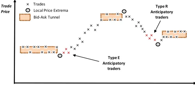
Figure 1 illustrates how we conceptualize the working of the price path algorithm and the relative location of anticipatory traders. The figure shows a sequence of trades (the “x’s”) for a portion of the day’s trading. There are periods with market-making activity in which non-price moving liquidity-based trading creates a bid-ask bounce sequence (shaded areas). When new information about the value of the asset arrives or liquidity demand changes, the market price reacts until the information is impounded in the price or new liquidity arrives to resolve the imbalance. Price reversals occur at the specified local price extrema (the circled trades).
In the figure, Type E traders possess the skills to process order flow and trade information to systematically forecast the short-term direction of trade prices. These participants react quickly after a price reversal occurs. Type R traders may use strategies that analyze order book liquidity or possess new information to place limit order prices near upcoming price reversals. The trades of these participants occur before but close to the local price extrema.
12 We also simulated our results with Type I and Type II error rates equal to 5%. These simulations gave a neighborhood size of 24 observations to maintain the type II error rate and a consistency parameter of approximately 63%.
14 B. Finding Anticipatory Traders
The WTI crude oil futures contract is among to most active contracts in futures markets. Thus, it has a large number of participants in any given expiration month. We use the False Discovery Rate (FDR) method of Benjamini and Hochberg (1995) as applied by Storey (2002) and Fishe and Smith (2012) to adjust for multiple testing problems.13 The FDR controls for the expected proportion of false discoveries in our sample. Specifically, as we increase the number of test statistics, we expect to increase the number of false rejections of the null. By effectively adjusting the critical levels for the appropriate test statistic, the FDR method limits these expected mistakes to a pre-specified proportion of successful statistics. We use a 5 percent control rate for this fraction. The FDR method increases the hurdle level and gives greater confidence that the participants we identify as anticipatory traders are truly either Type E or Type R traders.
We use a volume metric to determine whether a trader may be classified as participating early or late in a price path. Let be the quantity traded by participant i at time t in the vector of all trades ( ) on price path j. If participant i is a buyer (seller) at time t in path j then If participant i does not trade at time t in path j then . The heaviside function, defines whether trade arises in the first dth percentile of path j’s volume. The heaviside function equals 1 if the trade is in the first dth percentile and equals zero otherwise. The price direction along path j is defined to be
13 Recent applications of FDR include Barras, Scaillet, and Wermers (2010) who sought to identify fund managers with positive alpha performance, Bajgrowicz and Scaillet (2012) who examine the success of technical trading rules, Fishe and Smith (2012) who identified the number of informed traders in several futures contracts, and Harvey, Liu, and Zhu (2014) who examine threshold critical values necessary to claim a new risk factor after hundreds of asset pricing tests by previous researchers.
15
increasing (decreasing) if , where the first and last trade prices on the path are used to compute this difference.
Participants are identified as successful Type E traders on a given path if their trades occur in the first dth percentile of path volume and their trades are on the correct side for the path’s price change. For a given value of d, we compute the sample frequency of successes for each participant:
, (1)
where 1( ) is the binary indicator function based on the given expression, Tj is the number of
trades on path j, and J is the number of price paths in the sample.
To determine the null hypothesis, consider what may arise for traders who are not attempting to compute turning points for intraday prices. If a trader is randomly placing both buys and sells during the day in small sizes, then across all paths we might expect to find about 10% of these trades in the first 10% of path volume with d = 10. But how many of these are expected to be successful, meaning that they are aligned with the price path direction? The answer depends on how volume is distributed across up and down paths as well as how a trader mixes order size and side (e.g., buy or sell sides). If volume is approximately equally distributed between up and down paths, order sizes are small, and order sides are about equal in number during the day, then a null of 5% may be appropriate for our tests. However, volume is on average higher in down paths, traders often vary order sizes, and many traders end up with an unequal numbers of buys and sells. Such differences will alter the relevant null hypothesis.
16
Rather than seek a general solution for such nuances, we back up a step and impose a more restrictive condition in our tests. The measure in equation (1) is a statistic indicating the proportion of participant i’s trades that were executed in the first dth percentile of volume and were in the correct price direction. This proportion is conditional on our perfect foresight calculation of local price paths. If d = 10, then it is clear from how the price paths are created that a trader has a 10% chance of executing (buy or sell) within the first 10% of path volume assuming trades are randomly placed during the day. Any adjustments for order size or order side will lower this fraction. Thus, to make it more difficult to find successful anticipatory traders we use 10% as our null hypothesis. For each trader we test the null hypothesis,
. This is a binomial test and will have statistical power if a participant trades a sufficient number of times.
For our empirical work, we set d = 10 to identify Type E traders. To identify Type R traders, we consider the last 10th percentile of trading volume to be indicative of whether a trader uses information or foresight to anticipate the coming reversal of the price path. To measure success for Type R traders, we compute the proportion analogous to equation (1) using d = 90 to define the heaviside function:
. (2)
The null hypothesis that we test to identify Type R traders is . Note that to ensure statistical power, we confine our investigation to participants with more than 30 trades in our sample.
17
C. Inverse Regression and Anticipatory Trader Characteristics
We ask whether anticipatory traders are different from other participants in characteristics other than their trade placement along local price paths. Because the FDR method makes subsequent analyses conditional on the Type E and Type R groups, we use the inverse regression method to extract these characteristics.14 Consider the effects of a vector of exogenous variables ( ) on a binary dependent variable ( ) summarized as , where the subscript i denotes an observation index. Here the binary dependent variable indicates membership in either the Type E or the Type R group. We recognize the initial conditioning from the FDR method and seek to solve for , which requires a dimensional reduction. Fishe and Smith (2012) provide a detailed discussion of this reduction for the case of a binary dependent variable. Following their approach, assume a regression model:
(3)
where and is a coefficient in the parameter vector that belongs to a particular variable of interest ( ), with observations indexed by i. Then, the effects of for the identified participants may be measured by:
(4) where is a linear projection of the ith observation of the variable of interest using the least squares estimator of ; the latter is computed by regressing the variable of interest on all other exogenous variables in , which is labelled as . In this formulation, the least squares method serves to reduce the dimensionality of the problem.
For example, if the characteristic of interest is the average speed of trading and there is only an intercept term in the remaining vector ( ), then reduces to the average speed of
18
trading in the sample. The estimate of the net effects of being a type of anticipatory trader ( ) is from equation (4), which is the average trading speed of that group of anticipatory participants net of the average trading speed of all participants. In effect, the least squares projection serves as a reference point, so that we are measuring Type E or Type R characteristics relative to what would be predicted given the overall incidence of those characteristics in the sample.
IV.DATA
The data we examine are derived from audit trail files for the CME/Nymex WTI light sweet crude oil futures contract. The WTI contract is traded worldwide on the Globex and ClearPort electronic platforms. A trading session commences at 6:00 p.m. and concludes at 5:15 p.m. (EST) the next day. However, the majority of a session’s volume occurs during the open outcry period, which is from 9:00 a.m. to 2:30 p.m. (EST) on Monday through Friday. For the WTI contract each one cent move in price represents a $10 change in contract value, which provides leveraged returns even for relatively small changes in price.
A. Sample Information
Our sample covers the period from September 12, 2011 to November 18, 2011, the latter of which was the last day of trading for the December 2011 expiration. This period is selected based on the trading and open interest activity in the December 2011 contract. The December 2011 contract is traditionally the first or second most active month in the year. Beginning on September 12th, the December expiration becomes the 1st or 2nd highest open interest and is the 1st, 2nd, or 3rd highest volume going forward. On September 21st, this expiration becomes the second highest volume contract. On October 7th it is the highest open contract, and on Oct
19
18th it is the highest volume contract going forward. On November 16th to 18th the volume rank falls from 1st to 2nd, and then 5th on the last day of trading in the expiration.
These files contain all trades and orders posted, modified, and/or cancelled on the Nymex exchange. The trade prices that we study are from outright trades and also prices on the outright side if the other side is a spread trade. All spread-to-spread trades are excluded as they are only indicative of relative prices.
Because we use order book data, we limit our sessions to all trades and orders between 6:00 a.m. and 4:15 p.m. (EST), which is the time range provided for the order book information in the CFTC database. There are a total 48 trading days and 20,977 unique participant accounts Note that all account data are anonymous, so we do not know names or locations of these market participants.
In order to determine price paths using the SPRT method described above, we remove non-price forming trades from the sample, which are mainly transfers and offsets. We filter out spread trades where both sides are holding the spread. If one side of a spread trade is an outright, we keep that side’s price if it is for the December 2011 contract. After applying these filters, there are 6,736,520 buy and sell trades in the sample.
Table I provides sample statistics on the trading volume, number of participants, and order book data. The information is calculated across days in the sample. Volume is active in the WTI contract with an average of 356,645 contracts traded each day. There are in total 24,977 unique participants with trades in our data, with an average of 2,939 of them active in any given day. Out of the many participants in this market, the majority of them are using manual entry methods to place their orders. There are only 399 algorithmic traders on average each day or about 13.6% of the daily average. Participants will modify about 60.5% of the daily
20
average new orders and eventually cancel an average of 85.5% of those orders. These data also show that the WTI crude oil contract is traded in a nearly pure limit order market, with market orders on average only 0.5% of daily orders. In our analysis, we do not examine stop orders, offsets, transfer messages, or special order trade types, such as TAS (Trade at settlement) trades.
B. Measuring and Modeling Speed
There are several ways to measure and model speed. The autoregressive conditional durations models of Engle and Russell (1998) and the multi-fractal Markov models of Chen, Diebold, and Schorfheide (2013) focus on inter-trade durations. These empirical models often study the high persistence and over-dispersion of duration data. These models inherently capture the flow of bids and offers off of the order book without special regard to who is trading.
As our focus is on the participants’ characteristics, we seek to identify and measure individual durations. To compute individual durations, we identify the initial order submission time for every order in the sample and document the exit accounting for those orders. Specifically, there are three ways an order may exit the order book: (1) cancellation, (2) matching a counterparty for an execution, and (3) administrative action. We exclude orders canceled by administrative action. If an individual cancels, we measure duration as the difference between the time the Nymex received the cancel message and the initial confirmation time of the order. This duration may be considered the participant decision speed because it is based on the speed at which the participant acts and does not explicitly depend on flows onto the order book to find a match.
21
If a trade occurs, we measure duration as the difference between the time the Nymex confirms the trade message and the initial confirmation time of the order. This duration may be considered the individual execution ormatching engine speed because it depends on a host of factors that affect the order book, such as liquidity flows and new information about price, as well as the initial and subsequent decisions of the participant placing the order message, such as whether to modify the limit price or quantity.
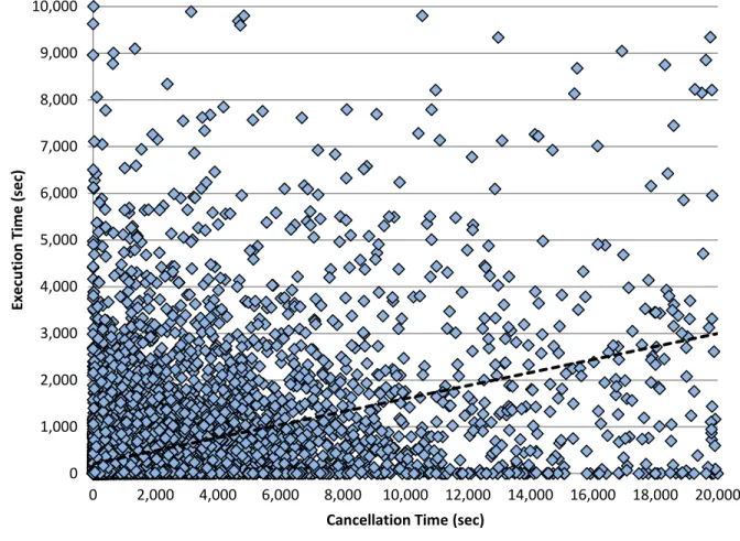
Figure 2 shows a comparison between participant cancellation and execution speeds. In this figure we have plotted the average values of these speeds for all participants in the sample. The plot is heavily populated near the origin, but there are many participants spread over the entire quadrant. In particular, there is a cluster of data points with low average cancellation speeds matched to higher average execution speeds and vice versa. In effect, some participants may have the capacity to act quite fast but their strategies result in slower execution speeds.
V. ANALYSIS
Our first task is to estimate local price paths in the WTI crude oil contract data. Then we use the FDR method to assess whether any participants can systematically trade in the correct direction either at the beginning of a price path or just before the next price reversal. After identifying such traders, we examine their characteristics relative to other traders, specifically decision speed and matching engine speed. Finally, we determine if the other traders react differently to the trades of anticipatory traders compared to how they react when such traders are not in the market.
22 A. Local Price Paths
We apply the SPRT method to find price paths for each day in the sample. Table 2 reports summary statistics derived from the calculation of these daily price paths. This table summarizes information by month and path direction and reports the average and median path returns in percent, average path duration in seconds, average path volume, average number of trades, and the average number of unique participants in a local price path. These statistics show that September had fewer paths and lower trading volume, which is expected as December was not the front month contract at this time. Trading activity and the number of paths increase markedly in October and November when the December expiration becomes the front month contract. These data do not show any strong patterns except that the “up” paths have lower average volume and somewhat shorter average path durations.
B. Identifying Anticipatory Participants
To provide statistical power to the FDR approach, we limit our analysis to a sub-sample of 7,871 participants who had 30 or more trades in the sample. This restriction removed 13,106 accounts, some of which may be anticipatory traders. Using the binomial statistic given by equation (1) in the FDR method, we found 112 participant accounts that indicated a systematic ability to trade in the first 10 percent of a given local path’s volume and to trade in the correct direction on that price path. These are all Type E traders. Using equation (2) in the FDR method, we identified 196 participant accounts that systematically executed trades during the last 10 percent of volume in the correct direction based on the subsequent price path. Within these two groups, we find that a total of 198 are algorithmic traders; 70 in the Type E group and 128 in the Type R group. The remaining traders use manual order entry methods.
23
Table III illustrates the effectiveness of the FDR method in identifying Type E and Type R traders, as well as how successful those traders are compared to other participants. The table shows the fraction of all trades on the buyside by Type E, Type R, and other traders in four volume segments within the local price paths, and also by the months in the sample. The four segments correspond to the first 10 percent of path volume, the next 40 percent to the volume midpoint, then the next 40 percent to the 90 percent level, and finally the last 10 percent of path volume. Panel A shows results for upward trending price paths and Panel B shows the same results for downward trending paths. In the first 10 percent of volume, Type E anticipatory traders are expected to disproportionately buy in upward trending paths and sell in downward trending paths. The data show an overwhelming tendency for this result with no less than an average of 82% of the trades on the buyside in the first volume segment for upward trending prices and between only 10% and 38% on the buyside in downward trending prices.
For type R traders, a similar effectiveness is found. In the last 10 percent of volume, Type R traders are expected to sell in upward trending price paths and buy in downward trending paths, thereby anticipating the change in local price direction in the next path. Table III shows that between 87% and 92% of the trades are on the buyside in the last volume segment for downward trending price paths. Similarly, between 5% and 12% of trades are on the buyside in the last segment for upward trending paths. These are compelling results given that the buyside percentages for other participants show no pattern different than a 50-50 split between buys and sells in these same volume segments.
Table III also shows trade count information for the different types of participants. The Type E and Type R traders execute only a small number of trades in September consistent
24
with the smaller path counts found during these months. These statistics suggest that anticipatory traders may be focused on the most active contract for implementing their strategies.
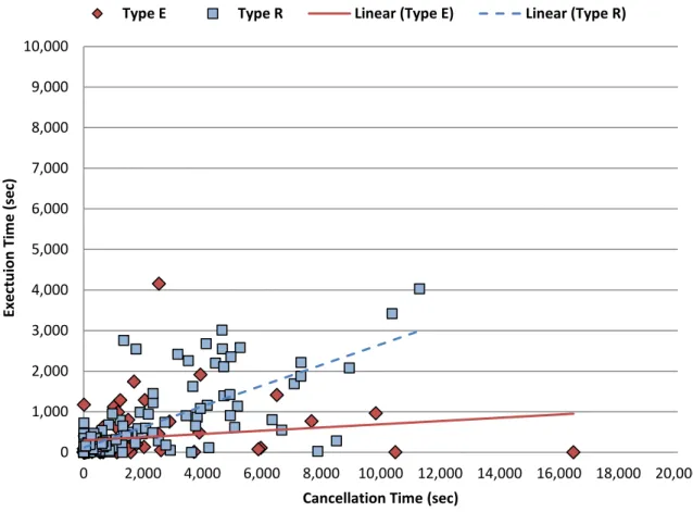
We are also interested in whether these anticipatory traders tend to be low latency or high frequency traders in the usual sense of the term. The Securities and Exchange Commission (2014) offers five criteria to identify high frequency traders: (1) high speed in routing and executing orders, (2) use of co-location services, (3) short time between establishing and liquidating positions, (4) using a submit and cancel approach to orders, and (5) ending trading sessions with near zero inventories. We have information on items (1), (3), and (4) from our calculation of average decision speeds from cancellation times and average matching speeds from execution times. A comparison of these speeds for Type E and Type R participants is shown in Figure 3.
From Figure 3, we see that several of the identified anticipatory traders are reasonably speedy, but the average times shown here are not on the order of 1-2 seconds as examined in previous studies. Visually, these traders appear to be a microcosm of the plot in Figure 2. The trend lines suggest that there is no linear connection between average execution matching speeds and average cancellation decision speeds for Type E traders, but there is a strong relationship for Type R traders where the trend line has an R-squared of 54.1%. It is possible that Type R traders use information gained from cancellations to influence when they execute a position.
Table IV provides additional evidence that almost no Type E traders, but possible a few Type R traders, can be considered analogous to what the literature calls HFTs. This table reports summary statistics from the CME/Nymex order book. Since July 2011, the CME has
25
required a binary flag on all orders submitted to its platform to identify whether an order is entered manually or electronically. A negative response means that the order is entered electronically, which then carries an automated trading system (ATS) label for that account. We report counts as well as the ATS order ratios for Type E, Type R, and other traders. The ATS order ratio is defined as the number of ATS orders divided by the total number of orders for a given trader group.
Panel A shows that a slight majority of the orders submitted by Type E traders are manual, with only 48.6% of their orders submitted electronically. In contrast, a much higher ratio of Type R traders orders are submitted electronically, 92.6%. Similar to Type R traders, the messages of other participants are dominated by electronic order submission with 92.8% of their orders marked as using an ATS. This strengthens the result that a few of the Type R traders can be HFTs.
Panel B of Table IV reports the distribution of messages by participant type. We observe that cancellation, execution, and modification rates differ significantly between Type E, Type R, and the rest of the market participants. Type E traders cancel very few orders when compared to everybody else. They also have a significantly higher order execution ratio, suggesting that they place their orders with the intention of execution, with little cancellations. Type R participants, on the other hand, have much higher modification rates compared to everyone else and lower execution rates. This suggests that they modify their orders a lot and few of those orders get executed.
Importantly, Panel C shows counts across trader types for those whose average decision and execution speeds are less than 0.5 seconds. Although we report counts in the teens for Type E and Type R execution speeds, these are driven by cases in which certain participants
26
use more market orders. For average decision speeds, there are no Type E participants and only three Type R participants revealing actions faster than 0.5 seconds. In contrast we find 75 high-speed participants among the remaining traders.15 These results confirm that the anticipatory trading we identify is not primarily a HFT phenomena.
C. Speed Characteristics
An important goal is to characterize the anticipatory participants in terms of speed. We follow two steps in this task. First, we specify an Anova model with characteristics partitioned by a set of dummy variables, some of which identify the anticipatory traders. With the Anova model, the effects of the anticipatory participants are measured relative to other omitted groups. In the second step, we implement the inverse regression approach to show the net effects of selected characteristics on anticipatory traders. Figure 2 and Table IV have shown that the population includes a heterogeneous mix of manual and ATS traders with varying speeds and types of messages. Thus, we choose several variables to characterize the Type E and Type R traders relative to other groups.
Table V shows regression results using participant decision speeds—measured from order cancellations—as the dependent variable. The transformation, natural logarithm of one plus the cancellation speed (in seconds with fractional milliseconds), is used in the regression. The variables, "First 10% of Path Volume", "Last 10% of Path Volume", and "Between 10% to 50% of Path Volume", indicate whether the cancellation message occurs during the first 10% of path volume, last 10%, or during the first half of volume that excludes the first 10%, respectively. The "Type E Trader" and "Type R Trader" variables indicate whether the trade is made by a Type E or Type R trader, respectively. Interaction terms are included in selected
15 Similar results are found if we compute decision speeds from order entry to an order modification, although the counts are lower because not all participants use modification strategies.
27
models: (1) Type E trader in the first 10% volume bin; (2) Type R trader in the last 10% volume bin; (3) Type E trader that is also algorithmic (ATS); and (4) Type R trader that is also algorithmic. Additional binary variables are "Modified Order" if there are any modification messages to the original order, "Proprietary trader" if the trade is made from a proprietary account, "Buy-Sell Indicator" which is one if this is a buy order, and the "Algorithmic Trader" variable which is one if this side of the trade was submitted by a computer algorithm. As all variables are binary, the intercept captures the omitted categories.
The p-values of these estimates are shown in parentheses below each coefficient. These are computed using heteroscedasticity-consistent standard errors. The adjusted R-squared for each model is also shown at the bottom of the table. The sample size is 30,870,516 observations.
The intercept term captures the average decision speed of the omitted group, which in the most general case (Model VI) is a non-anticipatory, non-proprietary, manual participant, cancelling during the 50-90% of path volume with no order modifications before the cancellation message. The average cancellation speed of the omitted group is 29.858 seconds, which decreases to an average of 4.388 seconds if these are algorithmic participants. The estimates in Models II-IV show that Type E and Type R participants are faster than the omitted group until we control for other order characteristics: proprietary trades, modifications, order side, and algorithmic variables. Adjusting for these features, Model VI shows that the average cancellation speed of manual Type E (Type R) traders is 91.579 (76.663) seconds. The interaction terms with the algorithmic variable show that Type E (Type R) traders are marginally faster that the omitted algorithmic group with an average
28
cancellation speed of 4.352 (4.090) seconds. From these estimates, the algorithmic trader coefficient is found to have the largest impact on average decision speed.
We reported above that Type E and Type R groups are composed of both manual and algorithmic traders and as Table V shows the average decision speeds of these traders are significantly different. Thus, it stands to reason that the capacity for speedy actions is per sé insufficient to define anticipatory trading. At least anticipatory trading as measured against our definition of local price paths.
Table V also includes regression estimates under the "Bootstrap" column heading. These estimates are averages of coefficient results from 1,500 random samples (with replacement) in which each trader account is chosen only once per sample. The purpose here is to equally weight each account in the Anova approach so that the volume from higher frequency participants does not give them greater influence on the resulting average comparisons. The 95% confidence intervals ("C.I.") from these simulations are shown below the average coefficient value. The sample size for each bootstrap sample is 11,869 observations.
The average coefficient signs and the confidence interval results generally confirm the comparisons using the full sample of data. However, the most notable difference is that the biggest effect on whether a participant’s decisions are speedy compared to other participants is the proprietary trading variable. That is, removing the volume influence of higher frequency traders, the algorithmic coefficient reduces its relative impact by 75%. As many manual traders may also be proprietary, these results suggest that some manual traders may operate at relatively fast decision speeds.
In fact, these data reveal that 32 manual traders have average cancellation speeds less than one second, with eleven of these less than one-half a second. More broadly, there are 100
29
manual traders with average cancellation speeds less than three seconds. Certainly, there are more algorithmic traders with these speeds as the comparable counts are 130 and 268, respectively. However the point is that some manual participants may use strategies that require quick actions, and some of these participants have that capacity.
Table VI presents similar speed results using the individual execution speed measure. In addition to the binary variables in Table V, we include a dummy variable for whether this participant was on the aggressive side of the trade. Model VI coefficient estimates show that manual Type E (9.50 sec) and Type R (24.71 sec) traders are on average slower than the base speed of the omitted group (4.88 sec), which now includes non-aggressive traders. Execution speed increases significantly in the first 10% of path volume for Type E traders, falling to 6.70 seconds for manual traders and from 3.95 to 2.63 seconds for algorithmic traders. These results suggest that when Type E traders detect that a path has a new local trend, they act quickly to execute directional positions. In contrast, average speeds decrease for Type R traders in the last 10% of path volume suggesting that strategies for these participants are not based a fast execution. Given their relatively high use of modifications (see Table IV), Type R traders appear to reposition their limit prices until they execute in the order flow near the end of a local price path.
The bootstrap results are also computed for individual execution speeds and shown in the last column in Table VI. These results confirm the execution speed profile of the Type R participants found when using the full sample. However, they suggest that the Type E participants may not be significantly faster that non-anticipatory participants, particularly in the first 10% of path volume when the data are not influenced by the volume from frequent
30
traders. In effect, those that act relatively fast in the first 10% of path volume are likely those who trade more than the average among the Type E participants.
We also estimated a logistic model (not shown) using the aggressor indicator as the dependent variable. The full sample results show that Type E traders (manual and algorithmic) are more aggressive than other participants and the probability of aggressive trades increases in the first 10% of path volume. The bootstrap estimates show that trader volume affects these observations as the previous claim holds only for algorithmic Type E participants with manual participants no more aggressive than other traders. Also, there is no aggressiveness effect in the first 10% of path volume in the bootstrap estimates. In contrast, the Type R traders are less likely to be aggressive that other participants, both for manual and algorithmic cases and this holds for the full sample and the bootstrap estimates. In short, higher volume, algorithmic Type E participants are more aggressive than other traders, but Type R participants are uniformly less aggressive.
The inverse regression results are presented in Table VII. As noted in the discussion of our methods above, these results show how the characteristics of Type E and Type R participants are different from what we would predict from the general distribution of those characteristics across the sample. The data in this table are for the sample of participants tested using the FDR method, so they all have 30 or more trades in the sample. As Type E and Type R findings are drawn from this group, their characteristics are defined similarly.
Table VII shows results for the following variables: average speed during the first 10% of path volume; average speed during the last 10% of path volume; average speed over all trades; average trade size; percentage of aggressive trades; percentage of trades on the buyside; binary indicator for proprietary trader; and a binary indicator for algorithmic trader. When a
31
participant has no data in either the first or last 10% of path volume, they are excluded from these regressions, so sample sizes vary between Type E and Type R results.
The speed results in Table VII are similar to the bootstrap findings for Table VI.16 Type E traders are found to be no different in speed than the general speed of sample, except when trading in the first 10% of path volume. Type R traders are slower than the sample average, but are not significantly slower during the last 10% of path volume. Thus, speed of execution is a distinguishing characteristic of Type E traders only when they detect a new price trend, otherwise they are similar to the sample average. Execution speed is a defining characteristic of Type R participants in that they are slower than would be expected from the sample data. These speed results suggest that Type E traders act quickly to execute orders when a new local price trend is detected, while Type R traders appear to modify their limit orders (see Table IV) in order to time their executions near the end of a price path. In the former case speed is important, but not significantly for the latter case.
Related to execution speed are the results for the algorithmic flag. Table VII shows that being algorithmic does not distinguish the Type E participant from the overall sample. This finding is consistent with the bootstrap results for the interaction between algorithmic trading and the first 10% of path volume in Table VI. However, algorithmic traders have significantly greater representation versus the overall sample for Type R traders, approximately 5.5% greater based on these estimates. We also isolated the algorithmic trader flag by excluding other variables and repeated the inverse regression procedure. The coefficient on this variable for the Type R group is 0.249 or 24.9%, which is significantly greater than the 18.3% sample average. Interestingly, because trading speed is not a distinguishing characteristic of Type R
16 The bootstrap findings are based on equal-weights for all participants, so they are most similar to these inverse regression results.
32
participants in the last 10% of path volume, being algorithmic appears to matter only for their trades elsewhere on a local path.
Other coefficient estimates in Table VII show characteristics that distinguish the Type E and Type R groups from the remaining participants. Both Type E and Type R traders have relatively larger trade sizes, which may explain why market participants can detect their activity as reported in the next section. Both groups also tend to be more represented on the buyside of the market. Lastly, Type E participants are more likely to be aggressive with their trades and Type R participants are more likely to be proprietary compared to the overall sample.
D. Measuring Effects on Other Market Participants
Our second goal is to determine whether other participants are affected by the trades of either Type E or Type R traders.17 Specifically, we want to know if other participants may reduce adverse selection costs by detecting such traders. Commonly, adverse selection costs are measured as a component of the bid-ask spread (Van Ness, Van Ness, and Warr, 2001; Barclay and Hendershott, 2004). Because we have order book data, we follow an alternative approach and investigate how anticipatory traders affect other participants by examining whether order cancellations and modifications by other participants are different in local price paths with anticipatory traders versus in paths without such traders. An obvious way to avoid or lower adverse selection costs if you can react quickly to such traders is to cancel or modify your order on the order book.
17 In a similar idea, Bernales (2014) presents a model of dynamic limit order markets with algorithmic traders. In his model, slow traders observe the fundamental value of an asset with a time lag and they can learn from market trading activity and improve the accuracy of their beliefs.
33
Thus, we examine whether the cancellations and order modifications of other participants later in a price path are correlated with the earlier trades of Type E and Type R participants. For Type E traders, we examine the activity of other participants in the path volume intervals: 10th to 50th percentile and the 10th to 100th percentile. For the Type R traders, we examine the 0 to 50th percentile and the 0 to 90th percentile of volume in the subsequent price path. We use regression methods adjusted appropriately for the time series characteristics of these data when analyzing cancellation and modification variables.
In Table VIII we measure the effects of Type E traders using their relative net buying behavior in the first 10% of current path volume and the effects of Type R traders using their relative net buying behavior in the last 10% of previous path volume. The relative net buying variable equals the buy minus sell volume of anticipatory traders divided by the total buy and sell volume of both anticipatory and other traders. These variables have zero values when there is no trading by Type E or Type R traders in these deciles. To correspond correctly, the dependent variables are all measured in the upper 90% of path volume in the Type E models and in the lower 90% of path volume in the next path following the path that measures Type R trading.
The dependent variable in Table VIII is the cancellation fraction for buyside orders for all other participants. This variable equals the volume of buy orders cancelled divided by the volume of both buy and sell orders cancelled for other participants. All of these variables are measured over the time corresponding to the relevant volume percentile. The other independent variables are the rate of price change over the current path and its lag value, the rate of trading over the current path and its lag value, and a dummy variable for path direction (one is for upward paths). The regressions are estimated after controlling for an AR(1) process