Understanding AIC and BIC in Model Selection
KENNETH P. BURNHAM DAVID R. ANDERSON
Colorado Cooperative Fish and Wildlife Research Unit (USGS-BRD)
The model selection literature has been generally poor at reflecting the deep foundations of the Akaike information criterion (AIC) and at making appropriate comparisons to the Bayesian information criterion (BIC). There is a clear philosophy, a sound criterion based in information theory, and a rigorous statistical foundation for AIC. AIC can be justified as Bayesian using a “savvy” prior on models that is a function of sample size and the number of model parameters. Furthermore, BIC can be derived as a non-Bayesian result. Therefore, arguments about using AIC versus BIC for model selection cannot be from a Bayes versus frequentist perspective. The philosophical context of what is assumed about reality, approximating models, and the intent of model-based infer-ence should determine whether AIC or BIC is used. Various facets of such multimodel inference are presented here, particularly methods of model averaging.
Keywords:AIC; BIC; model averaging; model selection; multimodel inference
1. INTRODUCTION
For a model selection context, we assume that there are data and a set of models and that statistical inference is to be model based. Clas-sically, it is assumed that there is a single correct (or even true) or, at least, best model, and that model suffices as the sole model for making inferences from the data. Although the identity (and para-meter values) of that model is unknown, it seems to be assumed that it can be estimated—in fact, well estimated. Therefore, classical infer-ence often involves a data-based search, over the model set, for (i.e., selection of ) that single correct model (but with estimated para-meters). Then inference is based on the fitted selected model as if it were the only model considered. Model selection uncertainty is
SOCIOLOGICAL METHODS & RESEARCH, Vol. 33, No. 2, November 2004 261-304 DOI: 10.1177/0049124104268644
© 2004 Sage Publications
ignored. This is considered justified because, after all, the single best model has been found. However, many selection methods used (e.g., classical stepwise selection) are not even based on an explicit criterion of what is a best model.
One might think the first step to improved inference under model selection would be to establish a selection criterion, such as the Akaike information criterion (AIC) or the Bayesian information cri-terion (BIC). However, we claim that the first step is to establish a philosophy about models and data analysis and then find a suitable model selection criterion. The key issue of such a philosophy seems to center on one issue: Are models ever true, in the sense that full real-ity is represented exactly by a model we can conceive and fit to the data, or are models merely approximations? Even minimally experi-enced practitioners of data analysis would surely say models are only approximations to full reality. Given this latter viewpoint, the issue is then really about whether the information (“truth”) in the data, as extractable by the models in the set, is simple (a few big effects only) or complex (many tapering effects). Moreover, there is a fundamen-tal issue of seeking parsimony in model fitting: What “size” of fitted model can be justified given the size of the sample, especially in the case of complex data (we believe most real data are complex)?
Model selection should be based on a well-justified criterion of what is the “best” model, and that criterion should be based on a phi-losophy about models and model-based statistical inference, includ-ing the fact that the data are finite and “noisy.” The criterion must be estimable from the data for each fitted model, and the criterion must fit into a general statistical inference framework. Basically, this means that model selection is justified and operates within either a likeli-hood or Bayesian framework or within both frameworks. Moreover, this criterion must reduce to a number for each fitted model, given the data, and it must allow computation of model weights to quan-tify the uncertainty that each model is the target best model. Such a framework and methodology allows us to go beyond inference based on only the selected best model. Rather, we do inference based on the full set of models: multimodel inference. Very little of the extensive model selection literature goes beyond the concept of a single best model, often because it is assumed that the model set contains the true model. This is true even for major or recent publications (e.g., Linhart and Zucchini 1986; McQuarrie and Tsai 1998; Lahiri 2001).
Two well-known approaches meet these conditions operationally: information-theoretic selection based on Kullback-Leibler (K-L) information loss and Bayesian model selection based on Bayes fac-tors. AIC represents the first approach. We will let the BIC approxima-tion to the Bayes factor represent the second approach; exact Bayesian model selection (see, e.g., Gelfand and Dey 1994) can be much more complex than BIC—too complex for our purposes here. The focus and message of our study is on the depth of the foundation underlying K-L information and AIC. Many people using, abusing, or refusing AIC do not know its foundations or its current depth of development for coping with model selection uncertainty (multimodel inference). Moreover, understanding either AIC or BIC is enhanced by contrast-ing them; therefore, we will provide contrasts. Another reason to include BIC here, despite AIC being our focus, is because by using the BIC approximation to the Bayes factor, we can show that AIC has a Bayesian derivation.
We will not give the mathematical derivations of AIC or BIC. Neither will we say much about the philosophy on deriving a prior set of models. Mathematical and philosophical background for our purposes is given in Burnham and Anderson (2002). There is much other relevant literature that we could direct the reader to about AIC (e.g., Akaike 1973, 1981; deLeeuw 1992) and Bayesian model selec-tion (e.g., Gelfand and Dey 1994; Gelman et al. 1995; Raftery 1995; Kass and Raftery 1995; Key, Pericchi, and Smith 1999; Hoeting et al. 1999). For an extensive set of references, we direct the reader to Burnham and Anderson (2002) and Lahiri (2001). We do not assume the reader has read all, or much, of this literature. However, we do assume that the reader has a general familiarity with model selection, including having encountered AIC and BIC, as well as arguments pro and con about which one to use (e.g., Weakliem 1999).
Our article is organized around the following sections. Section 2 is a careful review of K-L information; parsimony; AIC as an asymptotically unbiased estimator of relative, expected K-L informa-tion; AICcand Takeuchi’s information criterion (TIC); scaling crite-rion values (i); the discrete likelihood of modeli, given the data; Akaike weights; the concept of evidence; and measures of precision that incorporate model selection uncertainty. Section 3 is a review of the basis and application of BIC. Issues surrounding the assumption of a true model, the role of sample size in model selection when a
true model is assumed, and real-world issues such as the existence of tapering effect sizes are reviewed. Section 4 is a derivation of AIC as a Bayesian result; this derivation hinges on the use of a “savvy” prior on models. Often, model priors attempt to be noninformative; however, this practice has hidden and important implications (it is not innocent). Section 5 introduces several philosophical issues and com-parisons between AIC versus BIC. This section focuses additional attention on truth, approximating models of truth, and the careless notion of true models (mathematical models that exactly express full reality). Model selection philosophy should not be based on simple Bayesian versus non-Bayesian arguments. Section 6 compares the performance of AIC versus BIC and notes that many Monte Carlo sim-ulations are aimed only at assessing the probability of finding the true model. This practice misses the point of statistical inference and has led to widespread misunderstandings. Section 6 also makes the case for multimodel inference procedures, rather than making inference from only the model estimated to be best. Multimodel inference often lessens the performance differences between AIC and BIC selection. Finally, Section 7 presents a discussion of the more important issues and concludes that model selection should be viewed as a way to com-pute model weights (posterior model probabilities), often as a step toward model averaging and other forms of multimodel inference.
2. AIC: AN ASYMPTOTICALLY UNBIASED ESTIMATOR OF EXPECTED K-L INFORMATION
SCIENCE PHILOSOPHY AND THE INFORMATION-THEORETIC APPROACH
Information theorists do not believe in the notion of true models. Models, by definition, are only approximations to unknown reality or truth; there are no true models that perfectly reflect full reality. George Box made the famous statement, “All models are wrong but some are useful.” Furthermore, a “best model,” for analysis of data, depends on sample size; smaller effects can often only be revealed as sample size increases. The amount of information in large data sets (e.g.,n =3,500) greatly exceeds the information in small data sets (e.g.,n=22). Data sets in some fields are very large (terabytes), and
good approximating models for such applications are often highly structured and parameterized compared to more typical applications in which sample size is modest. The information-theoretic paradigm rests on the assumption that good data, relevant to the issue, are available, and these have been collected in an appropriate manner (Bayesians would want this also). Three general principles guide model-based inference in the sciences.
Simplicity and parsimony. Occam’s razor suggests, “Shave away all but what is necessary.” Parsimony enjoys a featured place in scientific thinking in general and in modeling specifically (see Forster and Sober 1994; Forster 2000, 2001 for a strictly science philo-sophy perspective). Model selection (variable selection in regression is a special case) is a bias versus variance trade-off, and this is the statistical principle of parsimony. Inference under models with too few parameters (variables) can be biased, while with models having too many parameters (variables), there may be poor precision or iden-tification of effects that are, in fact, spurious. These considerations call for a balance between under- and overfitted models—the so-called model selection problem (see Forster 2000, 2001).
Multiple working hypotheses. Chamberlin ([1890] 1965) advo-cated the concept of “multiple working hypotheses.” Here, there is no null hypothesis; instead, there are several well-supported hypothe-ses (equivalently, “models”) that are being entertained. The a priori “science” of the issue enters at this important stage. Relevant empiri-cal data are then gathered and analyzed, and it is expected that the results tend to support one or more hypotheses while providing less support for other hypotheses. Repetition of this general approach leads to advances in the sciences. New or more elaborate hypothe-ses are added, while hypothehypothe-ses with little empirical support are gradually dropped from consideration. At any one point in time, there are multiple hypotheses (models) still under consideration—the model set evolves. An important feature of this multiplicity is that the number of alternative models should be kept small; the analysis of, say, hundreds or thousands of models is not justified, except when prediction is the only objective or in the most exploratory phases of an investigation. We have seen applications in which more than a million models were fitted, even though the sample size was modest (60-200); we do not view such activities as reasonable.
Similarly, a proper analysis must consider the science context and cannot successfully be based on “just the numbers.”
Strength of evidence. Providing quantitative information to judge the “strength of evidence” is central to science. Null hypothesis testing only provides arbitrary dichotomies (e.g., significant vs. nonsignifi-cant), and in the all-too-often-seen case in which the null hypothesis is false on a priori grounds, the test result is superfluous. Hypothesis testing is particularly limited in model selection, and this is well docu-mented in the statistical literature. Royall (1997) provides an interest-ing discussion of the likelihood-based strength-of-evidence approach in simple statistical situations.
KULLBACK-LEIBLER INFORMATION
In 1951, S. Kullback and R. A. Leibler published a now-famous paper (Kullback and Leibler 1951) that quantified the meaning of “information” as related to R. A. Fisher’s concept of sufficient statistics. Their celebrated result, called Kullback-Leibler infor-mation, is a fundamental quantity in the sciences and has earlier roots back to Boltzmann’s concept of entropy (Boltzmann 1877). Boltzmann’s entropy and the associated second law of thermody-namics represents one of the most outstanding achievements of nineteenth-century science.
We begin with the concept thatf denotes full reality or truth;fhas no parameters (parameters are a human concept). We usegto denote an approximating model, a probability distribution. K-L information
I (f, g)is the information lost when modelgis used to approximate
f; this is defined for continuous functions as the integral
I (f, g)=f (x)log f (x) g(x|θ ) dx.
Clearly, the best model loses the least information relative to other models in the set; this is equivalent to minimizing I (f, g)over g. Alternatively, K-L information can be conceptualized as a “distance” between full reality and a model.
Full realityf is considered to be fixed, and only gvaries over a space of models indexed byθ. Of course, full reality is not a function of sample size n; truth does not change as nchanges. No concept
of a true model is implied here, and no assumption is made that the models must be nested.
The criterion I (f, g) cannot be used directly in model selection because it requires knowledge of full truth, or reality, and the para-metersθin the approximating models,gi(or, more explicitly,gi(x|θ )). In data analysis, the model parameters must be estimated, and there is often substantial uncertainty in this estimation. Models based on estimated parameters represent a major distinction from the case in which model parameters are known. This distinction affects how K-L information must be used as a basis for model selection and ranking and requires a change in the model selection criterion to that of min-imizing expected estimated K-L information rather than minmin-imizing known K-L information (over the set ofRmodels considered).
K-L information can be expressed as
I (f, g)=f (x)log(f (x))dx−f (x)log(g(x|θ ))dx,
or
I (f, g)=Ef[log(f (x))]−Ef[log(g(x|θ ))],
where the expectations are taken with respect to truth. The quantity
Ef[log(f (x))] is a constant (say,C) across models. Hence,
I (f, g)=C−Ef[log(g(x|θ ))], where
C =f (x)log(f (x))dx
does not depend on the data or the model. Thus, only relative expected K-L information, Ef[log(g(x|θ ))], needs to be estimated for each model in the set.
AKAIKE’S INFORMATION CRITERION (AIC)
Akaike (1973, 1974, 1985, 1994) showed that the critical issue for getting a rigorous model selection criterion based on K-L information was to estimate
where the inner part is justEf[log(g(x|θ ))], withθ replaced by the maximum likelihood estimator (MLE) of θ based on the assumed modelgand datay. Although onlyydenotes data, it is convenient to conceptualize bothxandyas independent random samples from the same distribution. Both statistical expectations are taken with respect to truth (f). This double expectation is the target of all model selection approaches based on K-L information (e.g., AIC, AICc, and TIC).
Akaike (1973, 1974) found a formal relationship between K-L information (a dominant paradigm in information and coding theory) and likelihood theory (the dominant paradigm in statistics) (see deLeeuw 1992). He found that the maximized log-likelihood value was a biased estimate of EyEx[log(g(x| ˆθ (y)))], but this bias was approximately equal toK, the number of estimable para-meters in the approximating model, g (for details, see Burnham and Anderson 2002, chap. 7). This is an asymptotic result of fun-damental importance. Thus, an approximately unbiased estimator of EyEx[log(g(x| ˆθ (y)))] for large samples and “good” models is log(L(θˆ|data)) –K. This result is equivalent to
log(L(θˆ|data))−K =C− ˆEθˆ[I (f,g)ˆ ], wheregˆ =g(·| ˆθ ).
This finding makes it possible to combine estimation (i.e., maxi-mum likelihood or least squares) and model selection under a uni-fied optimization framework. Akaike found an estimator of expected, relative K-L information based on the maximized log-likelihood func-tion, corrected for asymptotic bias:
relativeE(Kˆ -L)=log(L(θˆ|data))−K.
Kis the asymptotic bias correction term and is in no way arbitrary (as is sometimes erroneously stated in the literature). Akaike (1973, 1974) multiplied this simple but profound result by –2 (for “historical reasons”), and this became Akaike’s information criterion:
AIC= −2 log(L(θˆ|data))+2K.
In the special case of least squares (LS) estimation with normally distributed errors, AIC can be expressed as
where ˆ σ2 = (ˆi)2 n ,
and theˆi are the estimated residuals from the fitted model. In this case,Kmust be the total number of parameters in the model, including the intercept andσ2. Thus, AIC is easy to compute from the results of LS estimation in the case of linear models or from the results of a likelihood-based analysis in general (Edwards 1992; Azzalini 1996). Akaike’s procedures are now called information theoretic because they are based on K-L information (see Akaike 1983, 1992, 1994; Parzen, Tanabe, and Kitagawa 1998). It is common to find literature that seems to deal only with AIC as one of many types of criteria, without any apparent understanding that AIC is an estimate of some-thing much more fundamental: K-L information.
Assuming a set of a priori candidate models has been defined and is well supported by the underlying science, then AIC is computed for each of the approximating models in the set (i.e.,gi,i=1,2, . . . , R). Using AIC, the models are then easily ranked from best to worst based on the empirical data at hand. This is a simple, compelling concept, based on deep theoretical foundations (i.e., entropy, K-L informa-tion, and likelihood theory). Assuming independence of the sample variates, AIC model selection has certain cross-validation properties (Stone 1974, 1977).
It seems worth noting here that the large sample approximates the expected value of AIC (for a “good” model), inasmuch as this result is not given in Burnham and Anderson (2002). The MLEθ (y)ˆ con-verges, asngets large, to theθothat minimizes K-L information loss for modelg. Large-sample expected AIC converges to
E(AIC)= −2C+2I (f, g(·|θo))+K.
IMPORTANT REFINEMENTS: EXTENDED CRITERIA
Akaike’s approach allowed model selection to be firmly based on a fundamental theory and allowed further theoretical work. WhenK
is large relative to sample sizen (which includes when nis small, for anyK), there is a small-sample (second-order bias correction)
version called AICc,
AICc = −2 log(L(θ ))ˆ +2K+
2K(K +1) n−K−1
(see Sugiura 1978; Hurvich and Tsai 1989, 1995), and this should be used unlessn/K >about 40 for the model with the largest value ofK. A pervasive mistake in the model selection literature is the use of AIC when AICcreally should be used. Because AICcconverges to AIC, asngets large, in practice, AICcshould be used. People often conclude that AIC overfits because they failed to use the second-order criterion, AICc.
Takeuchi (1976) derived an asymptotically unbiased estimator of relative, expected K-L information that applies in general without assuming that model g is true (i.e., without the special conditions underlying Akaike’s derivation of AIC). His method (TIC) requires quite large sample sizes to reliably estimate the bias adjustment term, which is the trace of the product of two K-by-K matrices (i.e., tr[J (θo)I (θo)−1]; details in Burnham and Anderson 2002:65-66, 362-74). TIC represents an important conceptual advance and further justifies AIC. In many cases, the complicated bias adjustment term is approximately equal toK, and this result gives further credence to using AIC and AICc in practice. In a sense, AIC is a parsimo-nious approach to TIC. The large-sample expected value of TIC is
E(TIC)= −2C+2I (f, g(·|θo))+tr[J (θo)I (θo)−1].
Investigators working in applied data analysis have several power-ful methods for ranking models and making inferences from empiri-cal data to the population or process of interest. In practice, one need not assume that the “true model” is in the set of candidates (although this is sometimes mistakenly stated in the technical liter-ature on AIC). These information criteria are estimates of relative, expected K-L information and are an extension of Fisher’s likelihood theory (Akaike 1992). AIC and AICcare easy to compute and quite effective in a very wide variety of applications.
iVALUES
The individual AIC values are not interpretable as they contain arbitrary constants and are much affected by sample size (we have
seen AIC values ranging from –600 to 340,000). Here it is imperative to rescale AIC or AICcto
i =AICi −AICmin,
where AICminis the minimum of theRdifferent AICivalues (i.e., the minimum is ati = min). This transformation forces the best model to have = 0, while the rest of the models have positive values. The constant representing Ef[log(f (x))] is eliminated from these
i values. Hence,i is the information loss experienced if we are using fitted model gi rather than the best model, gmin, for infer-ence. Theseiallow meaningful interpretation without the unknown scaling constants and sample size issues that enter into AIC values.
Theiare easy to interpret and allow a quick strength-of-evidence comparison and ranking of candidate hypotheses or models. The larger the i, the less plausible is fitted modeli as being the best approximating model in the candidate set. It is generally important to know which model (hypothesis) is second best (the ranking), as well as some measure of its standing with respect to the best model. Some simple rules of thumb are often useful in assessing the relative merits of models in the set: Models havingi ≤2 have substantial support (evidence), those in which 4 ≤ i ≤ 7 have considerably less sup-port, and models havingi >10 have essentially no support. These rough guidelines have similar counterparts in the Bayesian literature (Raftery 1996).
Naive users often question the importance of ai =10 when the two AIC values might be, for example, 280,000 and 280,010. The difference of 10 here might seem trivial. In fact, large AIC values contain large scaling constants, while theiare free of such constants. Only these differences in AIC are interpretable as to the strength of evidence.
LIKELIHOOD OF A MODEL GIVEN THE DATA
The simple transformation exp(−i/2), for i = 1,2, . . . , R, provides the likelihood of the model (Akaike 1981) given the data: L(gi|data). (Recall that Akaike defined his AIC after multiplying through by –2; otherwise,L(gi|data) = exp(i) would have been the case, withredefined in the obvious way). This is a likelihood
function over the model set in the sense thatL(θ|data, gi) is the like-lihood over the parameter space (for modelgi) of the parameterθ, given the data (x) and the model (gi).
The relative likelihood of model i versus modelj isL(gi|data)/ L(gj|data); this is termed theevidence ratio, and it does not depend on any of the other models under consideration. Without loss of gen-erality, we may assume that modelgiis more likely thangj. Then, if this evidence ratio is large (e.g.,>150 is quite large), modelgj is a poor model relative to modelgi, based on the data.
AKAIKE WEIGHTS,wi
It is convenient to normalize the model likelihoods such that they sum to 1 and treat them as probabilities; hence, we use
wi =
exp(−i/2)
R
r=1exp(−r/2)
.
Thewi, called Akaike weights, are useful as the “weight of evi-dence” in favor of modelgi(·|θ )as being the actual K-L best model in the set (in this context, a model,g, is considered a “parameter”). The ratios wi/wj are identical to the original likelihood ratios, L(gi|data)/L(gj|data), and so they are invariant to the model set, but the wi values depend on the full model set because they sum to 1. However,wi, i =1, . . . , Rare useful in additional ways. For exam-ple, thewi are interpreted as the probability that modeliis, in fact, the K-L best model for the data (strictly under K-L information the-ory, this is a heuristic interpretation, but it is justified by a Bayesian interpretation of AIC; see below). This latter inference about model selection uncertainty is conditional on both the data and the full set of a priori models considered.
UNCONDITIONAL ESTIMATES OF PRECISION, A TYPE OF MULTIMODEL INFERENCE
Typically, estimates of sampling variance are conditional on a given model as if there were no uncertainty about which model to use (Breiman called this a “quiet scandal”; Breiman 1992). When model selection has been done, there is a variance component due to model selection uncertainty that should be incorporated into estimates of
precision. That is, one needs estimates that are “unconditional” on the selected model. A simple estimator of the unconditional variance for the maximum likelihood estimatorθˆfrom the selected (best) model is
var(θ )ˆ¯ = R i=1 wi[var(θˆi|gi)+(θˆi − ˆ¯θ )2]1/2 2 , (1) where ˆ¯ θ = R i=1 wiθˆi,
andθˆ¯represents a form of “model averaging.” The notationθˆi here means that the parameter θ is estimated based on model gi, butθ is a parameter in common to allRmodels (even if its value is 0 in model k, so then we use θˆk = 0). This estimator, from Buckland, Burnham, and Augustin (1997), includes a term for the conditional sampling variance, given modelgi(denoted asvar(θˆi|gi)here), and a variance component for model selection uncertainty,(θˆi− ˆ¯θ )2. These variance components are multiplied by the Akaike weights, which reflect the relative support, or evidence, for modeli. Burnham and Anderson (2002:206-43) provide a number of Monte Carlo results on achieved confidence interval coverage when information-theoretic approaches are used in some moderately challenging data sets. For the most part, achieved confidence interval coverage is near the nominal level. Model averaging arises naturally when the uncondi-tional variance is derived.
OTHER FORMS OF MULTIMODEL INFERENCE
Rather than base inferences on a single, selected best model from an a priori set of models, inference can be based on the entire set of models. Such inferences can be made if a parameter, sayθ, is in common over all models (asθiin modelgi) or if the goal is prediction. Then, by using the weighted average for that parameter across models (i.e.,θˆ¯ =wiθˆi), we are basing point inference on the entire set of models. This approach has both practical and philosophical advan-tages. When a model-averaged estimator can be used, it often has a
more honest measure of precision and reduced bias compared to the estimator from just the selected best model (Burnham and Anderson 2002, chaps. 4–6). In all-subsets regression, we can consider that the regression coefficient (parameter) βp for predictor xp is in all the models, but for some models,βp = 0(xp is not in those models). In this situation, if model averaging is done over all the models, the resultant estimator βp has less model selection bias than βˆp taken from the selected best model (Burnham and Anderson 2002:151-3, 248-55).
Assessment of the relative importance of variables has often been based only on the best model (e.g., often selected using a stepwise test-ing procedure). Variables in that best model are considered “impor-tant,” while excluded variables are considered not important. This is too simplistic. Importance of a variable can be refined by mak-ing inference from all the models in the candidate set (see Burnham and Anderson 2002, chaps. 4–6). Akaike weights are summed for all models containing predictor variablexj, j =1, . . . , R; denote these sums as w+(j ). The predictor variable with the largest predictor weight, w+(j ), is estimated to be the most important; the variable with the smallest sum is estimated to be the least important predictor. This procedure is superior to making inferences concerning the rel-ative importance of variables based only on the best model. This is particularly important when the second or third best model is nearly as well supported as the best model or when all models have nearly equal support. (There are “design” considerations about the set of models to consider when a goal is assessing variable importance. We do not discuss these considerations here—the key issue is one of balance of models with and without each variable.)
SUMMARY
At a conceptual level, reasonable data and a good model allow a separation of “information” and “noise.” Here, informationrelates to the structure of relationships, estimates of model parameters, and components of variance.Noise, then, refers to the residuals: variation left unexplained. We want an approximating model that minimizes information loss,I (f, g), and properly separates noise (noninforma-tion or entropy) from structural informa(noninforma-tion. In a very important sense,
we are not trying to model the data; instead, we are trying to model the information in the data.
Information-theoretic methods are relatively simple to understand and practical to employ across a very large class of empirical situa-tions and scientific disciplines. The methods are easy to compute by hand if necessary, assuming one has the parameter estimates, the con-ditional variancesvar(θˆi|gi), and the maximized log-likelihood values for each of theRcandidate models from standard statistical software. Researchers can easily understand the heuristics and application of the information-theoretic methods; we believe it is very important that people understand the methods they employ. Information-theoretic approaches should not be used unthinkingly; a good set of a priori models is essential, and this involves professional judgment and inte-gration of the science of the issue into the model set.
3. UNDERSTANDING BIC
Schwarz (1978) derived the Bayesian information criterion as BIC= −2 ln(L)+Klog(n).
As usually used, one computes the BIC for each model and selects the model with the smallest criterion value. BIC is a misnomer as it is not related to information theory. As withAICi, we defineBICias the difference of BIC for modelgiand the minimum BIC value. More complete usage entails computing posterior model probabilities,
pi, as pi =Pr{gi|data} = exp(−12BICi) R r=1exp(− 1 2BICr)
(Raftery 1995). The above posterior model probabilities are based on assuming that prior model probabilities are all 1/R. Most applications of BIC use it in a frequentist spirit and hence ignore issues of prior and posterior model probabilities.
The model selection literature, as a whole, is confusing as regards the following issues about BIC (and about Bayesian model selection in general):
1. Does the derivation of BIC assume the existence of a true model, or, more narrowly, is the true model assumed to be in the model set when using BIC? (Schwarz’s derivation specified these conditions.) 2. What do the “model probabilities” mean? That is, how should we
interpret them vis-`a-vis a “true” model?
Mathematically (we emphasizemathematicalhere), for an iid sam-ple and a fixed set of models, there is a model—say, modelgt—with posterior probabilitypt such that asn → ∞, thenpt → 1 and all otherpr → 0. In this sense, there is a clear target model that BIC “seeks” to select.
3. Does the above result mean modelgtmust be the true model?
The answers to questions 1 and 3 are simple: no. That is, BIC (as the basis for an approximation to a certain Bayesian integral) can be derived without assuming that the model underlying the deriva-tion is true (see, e.g., Cavanaugh and Neath 1999; Burnham and Anderson 2002:293-5). Certainly, in applying BIC, the model set need not contain the (nonexistent) true model representing full reality. Moreover, the convergence in probability of the BIC-selected model to a target model (under the idealization of an iid sample) does not logically mean that that target model must be the true data-generating distribution.
The answer to question 2 involves characterizing the target model to which the BIC-selected model converges. That model can be char-acterized in terms of the values of the K-L discrepancy andKfor the set of models. For modelgr, the K-L “distance” of the model from the truth is denotedI (f, gr). Often,gr ≡gr(x|θ )would denote a para-metric family of models forθ ∈ , withbeing aKr-dimensional space. However, we takegr generally to denote the specific family member for the unique θo ∈ , which makes gr, in the family of models, closest to the truth in K-L distance. For the family of models
gr(x|θ ),θ ∈, asn→ ∞(with iid data), the MLE, and the Bayesian point estimator of θ converge to θo. Thus, asymptotically, we can characterize the particular model thatgr represents: gr ≡ gr(x|θo) (for details, see Burnham and Anderson 2002 and references cited therein). Also, we have the set of corresponding minimized K-L dis-tances:{I (f, gr), r =1, . . . , R}. For an iid sample, we can represent these distances asI (f, gr) = nI1(f, gr), where theI1(f, gr)do not
depend on sample size (they are forn=1). The point of this repre-sentation is to emphasize that the effect of increasing sample size is to scale up these distances.
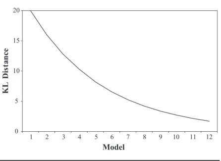
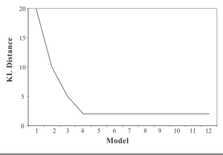
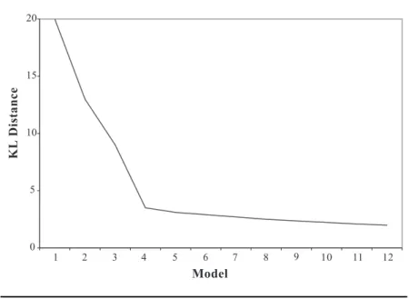
We may assume, without loss of generality, that these models are indexed worst (g1) to best (gR) in terms of their K-L distance and dimension Kr; hence, I (f, g1) ≥ I (f, g2) ≥ · · · ≥ I (f, gR). Figures 1 through 3 show three hypothetical scenarios of how these ordered distances might appear forR= 12 models, for unspecified
n(sincenserves merely to scale they-axis). LetQbe the tail-end subset of the so-ordered models, defined by {gr, r ≥ t,1 ≤ t ≤
R|I (f, gt−1) > I (f, gt) = · · · = I (f, gR)}. Set Qexists because
t =R(andt =1) is allowed, in which case the K-L best model (of theRmodels) is unique. For the case when subsetQcontains more than one model (i.e., 1≤t < R), then all of the models in this sub-set have the same K-L distance. Therefore, we further assume that models gt togR are ordered such thatKt < Kt+1 ≤ · · · ≤ KR (in principle,Kt =Kt+1could occur).
Thus, model gt is the most parsimonious model of the subset of models that are tied for the K-L best model. In this scenario (iid sample, fixed model set,n→ ∞), the BIC-selected model converges with probability 1 to modelgt, andptconverges to 1. However, unless
I (f, gt)=0, modelgtis not identical tof (nominally considered as truth), so we call it a quasi-true model. The only truth here is that in this model set, modelsgt+1togRprovide no improvement over model
gt—they are unnecessarily general (independent of sample size). The quasi-true model in the set of R models is the most parsimonious model that is closest to the truth in K-L information loss (model 12 in Figures 1 and 3, model 4 in Figure 2).
Thus, the Bayesian posterior model probabilitypr is the inferred probability that model gr is the quasi-true model in the model set. For a “very large” sample size, modelgtis the best model to use for inference. However, for small or moderate sample sizes obtained in practice, the model selected by BIC may be much more parsimonious than modelgt, especially if the quasi-true model is the most general model,gR, as in Figure 1. The concern for realistic sample sizes, then, is that the BIC-selected model may be underfit at the givenn. The model selected by BIC approaches the BIC target model from below, as nincreases, in terms of the ordering we imposed on the model
Model KL Dis ta n ce
Figure 1: Values of Kullback-Leibler (K-L) Information Loss,I(f,gr(·|θo)) ≡ nI1 (f,gr(·|θo)), Illustrated Under Tapering Effects for 12 Models Ordered by Decreasing K-L Information
NOTE: Sample sizen, and hence they-axis is left unspecified; this scenario favors Akaike information criterion (AIC)–based model selection.
set. This selected model can be quite far from the BIC theoretical target model at sample sizes seen in practice when tapering effects are present (Figure 1). The situation in which BIC performs well is that shown in Figure 2, with suitably largen.
Moreover, the BIC target model does not depend on sample sizen. However, we know that the number of parameters we can expect to reliably estimate from finite data does depend onn. In particular, if the set of ordered (large to small) K-L distances shows tapering effects (Figure 1), then a best model for making inference from the data may well be a more parsimonious model than the BIC target model (g12 in Figure 1), such as the best expected estimated K-L model, which is the AIC target model. As noted above, the target model for AIC is the model that minimizesEf[I (f, gr(·| ˆθ ))], r = 1, . . . , R. This target model is specific for the sample size at hand; hence, AIC seeks
0 5 10 15 20 Model KL Distance
Figure 2: Values of Kullback-Leibler (K-L) Information Loss,I(f,gr(·|θo)) ≡ nI1 (f,gr(·|θo)), Illustrated When Models 1 (Simplest) to 12 (Most General) Are Nested With Only a Few Big Effects
NOTE: Model 4 is a quasi-true model, and Models 5 to 12 are too general. Sample sizen, and hence they-axis is left unspecified; this scenario favors Bayesian information criterion (BIC)– based model selection.
a best model as its target, wherebestis heuristically a bias-variance trade-off (not a quasi-true model).
In reality, one can only assert that BIC model selection is asymp-totically consistent for the (generally) unique quasi-true model in the set of models. But that BIC-selected model can be quite biased at not-largenas an estimator of its target model. Also, from an infer-ence point of view, observing thatpt is nearly 1 does not justify an inference that modelgt is truth (such a statistical inference requires an a priori certainty that the true model is in the model set). This issue is intimately related to the fact that only differences such as
I (f, gr)−I (f, gt) are estimable from data (these K-L differences are closely related to AICr – AICt differences, hence to the ). Hence, with model selection, the effect is that sometimes people are erroneously lulled into thinking (assuming) that I (f, gt) is 0 and
hence thinking that they have found (the model for) full reality. These fitted models sometimes have seven or fewer parameters; surely, full reality cannot be so simple in the life sciences, economics, medicine, and the social sciences.
4. AIC AS A BAYESIAN RESULT
BIC model selection arises in the context of a large-sample approxi-mation to the Bayes factor, conjoined with assuming equal priors on models. The BIC statistic can be used more generally with any set of model priors. Letqibe the prior probability placed on modelgi. Then the Bayesian posterior model probability is approximated as
Pr{gi|data} = exp(−12BICi)qi R r=1exp(− 1 2BICr)qr
(this posterior actually depends on not just the data but also on the model set and the prior distribution on those models). Akaike weights can be easily obtained by using the model priorqias proportional to
exp 1 2BICi .exp −1 2AICi . Clearly, exp −1 2BICi .exp 1 2BICi .exp −1 2AICi =exp −1 2AICi .
Hence, with the implied prior probability distribution on models, we get pi =Pr{gi|data} = exp(−12BICi)qi R r=1exp(− 1 2BICr)qr = exp(− 1 2AICi) R r=1exp(− 1 2AICr) =wi, which is the Akaike weight for modelgi.
This prior probability on models can be expressed in a simple form as qi =C . exp 1 2Kilog(n)−Ki , (2) where C = R 1 r=1exp( 1 2Krlog(n)−Kr) . (3)
Thus, formally, the Akaike weights from AIC are (for large samples) Bayesian posterior model probabilities for this model prior (more details are in Burnham and Anderson 2002:302-5).
Given a model g(x|θ ), the prior distribution on θ will not and should not depend on sample size. This is very reasonable. Probably following from this line of reasoning, traditional Bayesian thinking about the prior distribution on models has been thatqr, r=1, . . . , R would also not depend onnorKr. This approach is neither necessary nor reasonable. There is limited information in a sample, so the more parameters one estimates, the poorer the average precision becomes for these estimates. Hence, in considering the prior distribution q
on models, we must consider the context of what we are assuming about the information in the data, as regards parameter estimation, and the models as approximations to some conceptual underlying “full-truth” generating distribution. Whileqr =1/Rseems reasonable and innocent, it is not always reasonable and is never innocent; that is, it implies that the target model is truth rather than a best approximating model, given that parameters are to be estimated. This is an important and unexpected result.
It is useful to think in terms of effects, for individual parameters, as|θ|/se(θ )ˆ . The standard error depends on sample size; hence, effect size depends on sample size. We would assume for such effects that few or none are truly zero in the context of analysis of real data from complex observational, quasi-experimental, or experimental studies (i.e., Figure 1 applies). In the information-theoretic spirit, we assume meaningful, informative data and thoughtfully selected predictors and models (not all studies meet these ideals). We assume tapering effects: Some may be big (values such as 10 or 5), but some are only 2, 1, 0.5, or less. We assume we can only estimaten/m parameters reliably;
mmight be 20 or as small as 10 (but surely,m 1 andm100). (In contrast, in the scenario in which BIC performs better than AIC, it is assumed that there are a few big effects defining the quasi-true model, which is itself nested in several or many overly general models; i.e., Figure 2 applies).
These concepts imply that the size (i.e.,K) of the appropriate model to fit the data should logically depend onn. This idea is not foreign to the statistical literature. For example, Lehman (1990:160) attributes to R. A. Fisher the quote, “More or less elaborate forms will be suit-able according to the volume of the data.” Using the notationk0for the optimalK, Lehman (1990) goes on to say, “The value ofk0will tend to increase as the number of observations increases and its determina-tion thus constitutes implementadetermina-tion of Fisher’s suggesdetermina-tion” (p. 162). Williams (2001) states, “We CANNOT ignore the degree of resolu-tion of the experiment when choosing our prior” (p. 235).
These ideas have led to a model prior wherein conceptually,
qr should depend onnandKr. Such a prior (class of priors, actually) is called asavvy prior. A savvy (definition: shrewdly informed) prior is logical under the information-theoretic model selection paradigm. We will call the savvy prior on models given by
qi =C.exp
1
2Kilog(n)−Ki
(formula 3b givesC) the K-L model prior. It is unique in terms of pro-ducing the AIC as approximately a Bayesian procedure (approximate only because BIC is an approximation).
Alternative savvy priors might be based on distributions such as a modified Poisson (i.e., applied to only Kr, r = 1, . . . , R), with expectedK set to ben/10. We looked at this idea in an all-subsets selection context and found that the K-L model prior produces a more spread-out (higher entropy) prior as compared to such a Poisson-based savvy prior when both produced the sameE(K). We are not wanting to start a cottage industry of seeking a best savvy prior because model-averaged inference seems very robust to model weights when those weights are well founded (as is the case for Akaike weights).
The full implications of being able to interpret AIC as a Bayesian result have not been determined and are an issue outside the scope of this study. It is, however, worth mentioning that the model-averaged
Bayesian posterior is a mixture distribution of each model-specific posterior distribution, with weights being the posterior model prob-abilities. Therefore, for any model-averaged parameter estimator, particularly for model-averaged prediction, alternative variance and covariance formulas are
var(θ )ˆ¯ = R i=1 wi[var(θˆi|gi)+(θˆi− ˆ¯θ )2], (4) cov(θ ,ˆ¯ τ )ˆ¯ = R i=1 wi[cov(θˆi,τˆi|gi)+(θˆi − ˆ¯θ )(τˆi− ˆ¯τ )]. (5) The formula given in Burnham and Anderson (2002:163-4) for such an unconditional covariance is ad hoc; hence, we now recom-mend the above covariance formula. We have rerun many simulations and examples from Burnham and Anderson (1998) using variance formula (4) and found that its performance is almost identical to that of the original unconditional variance formula (1) (see also Burnham and Anderson 2002:344-5). Our pragmatic thought is that it may well be desirable to use formula (4) rather than (1), but it is not necessary, except when covariances (formula 5) are also computed.
5. RATIONAL CHOICE OF AIC OR BIC
FREQUENTIST VERSUS BAYESIAN IS NOT THE ISSUE
The model selection literature contains, de facto, a long-running debate about using AIC or BIC. Much of the purely mathematical or Bayesian literature recommends BIC. We maintain that almost all the arguments for the use of BIC rather than AIC, with real data, are flawed and hence contribute more to confusion than to understand-ing. This assertion by itself is not an argument for AIC or against BIC because there are clearly defined contexts in which each method outperforms the other (Figure 1 or 2 for AIC or BIC, respectively).
For some people, BIC is strongly preferred because it is a Bayesian procedure, and they think AIC is non-Bayesian. However, AIC model selection is just as much a Bayesian procedure as is BIC selection. The difference is in the prior distribution placed on the model set.
Hence, for a Bayesian procedure, the argument about BIC versus AIC must reduce to one about priors on the models.
Alternatively, both AIC and BIC can be argued for or derived under a non-Bayesian approach. We have given above the arguments for AIC. When BIC is so derived, it is usually motivated by the mathe-matical context of nested models, including a true model simpler than the most general model in the set. This corresponds to the context of Figure 2, except with the added (but not needed) assumption that
I (f, gt) =0. Moreover, the goal is taken to be the selection of this true model, with probability 1 asn→ ∞(asymptotic consistency or sometimes dimension consistency).
Given that AIC and BIC model selection can both be derived as either frequentist or Bayesian procedures, one cannot argue for or against either of them on the basis that it is or is not Bayesian or non-Bayesian. What fundamentally distinguishes AIC versus BIC model selection is their different philosophies, including the exact nature of their target models and the conditions under which one outperforms the other for performance measures such as predictive mean square error. Thus, we maintain that comparison, hence selection for use, of AIC versus BIC must be based on comparing measures of their perfor-mance under conditions realistic of applications. (A now-rare version of Bayesian philosophy would deny the validity of such hypothetical frequentist comparisons as a basis for justifying inference methodo-logy. We regard such nihilism as being outside of the evidential spirit of science; we demand evidence.)
DIFFERENT PHILOSOPHIES AND TARGET MODELS
We have given the different philosophies and contexts in which the AIC or BIC model selection criteria arise and can be expected to perform well. Here we explicitly contrast these underpinnings in terms of K-L distances for the model set{gr(x|θo), r = 1, . . . , R}, with reference to Figures 1, 2, and 3, which represent I (f, gr) =
nI1(f, gr). Sample size nis left unspecified, except that it is large relative toKR, the largest value ofKr, yet of a practical size (e.g.,
KR =15 andn=200).
Given that the model parameters must be estimated so that parsi-mony is an important consideration, then just by looking at Figure 1,
we cannot say what is the best model to use for inference as a model fitted to the data. Model 12, as g12(x|θo) (i.e., at θ being the K-L distance-minimizing parameter value infor this class of models), is the best theoretical model, butg12(x| ˆθ )may not be the best model for inference. Model 12 is the target model for BIC but not for AIC. The target model for AIC will depend onnand could be, for example, Model 7 (there would be annfor which this would be true).
Despite that the target of BIC is a more general model than the target model for AIC, the model most often selected here by BIC will be less general than Model 7 unlessnis very large. It might be Model 5 or 6. It is known (from numerous papers and simulations in the literature) that in the tapering-effects context (Figure 1), AIC performs better than BIC. If this is the context of one’s real data analysis, then AIC should be used.
A very different scenario is given by Figure 2, wherein there are a few big effects, all captured by Model 4 (i.e.,g4(x|θo)), and Models 5 to 12 do not improve at all on Model 4. This scenario generally corresponds with Model 4 being nested in Models 5 to 12, often as part of a full sequence of nested models,gi ⊂gi+1. The obvious target model for selection is Model 4; Models 1 to 3 are too restrictive, and models in the class of Models 5 to 12 contain unneeded parameters (such parameters are actually zero). Scenarios such as that in Figure 2 are often used in simulation evaluations of model selection, despite that they seem unrealistic for most real data, so conclusions do not logically extend to the Figure 1 (or Figure 3) scenario.
Under the Figure 2 scenario and for sufficiently largen, BIC often selects Model 4 and does not select more general models (but may select less general models). AIC will select Model 4 much of the time, will tend not to select less general models, but will sometimes select more general models and do so even ifnis large. It is this scenario that motivates the model selection literature to conclude that BIC is consistent and AIC is not consistent. We maintain that this conclu-sion is for an unrealistic scenario with respect to a lot of real data as regards the pattern of the K-L distances. Also ignored in this conclusion is the issue that for real data, the model set itself should change as sample size increases by orders of magnitude. Also, infer-entially, such “consistency” can only imply a quasi-true model, not truth as such.
0 5 10 15 20 Model KL Distance
Figure 3: Values of Kullback-Leibler (K-L) Information Loss,I(f,gr(·|θo)) ≡ nI1 (f,gr(·|θo)), Illustrated When Models 1 (Simplest) to 12 (Most General) Are Nested With a Few Big Effects (Model 4), Then Much Smaller Tapering Effects (Models 5-12)
NOTE: Whether the Bayesian information criterion (BIC) or the Akaike information criterion (AIC) is favored depends on sample size.
That reality could be as depicted in Figure 2 seems strained, but it could be as depicted in Figure 3 (as well as Figure 1). The latter scenario might occur and presents a problematic case for theoretical analysis. Simulation seems needed there and, in general, to evaluate model selection performance under realistic scenarios. For Figure 3, the target model for BIC is also Model 12, but Model 4 would likely be a better choice at moderate to even large sample sizes.
FULL REALITY AND TAPERING EFFECTS
Often, the context of data analysis with a focus on model selection is one of many covariates and predictive factors (x). The conceptual truth underlying the data is about what is the marginal truth just for
this context and these measured factors. If this truth, conceptually asf (y|x), implies thatE(y|x) has tapering effects, then any fitted good model will need tapering effects. In the context of a linear model, and for an unknown (to us) ordering of the predictors, then for E(y|x) = β0 + β1x1 + · · · βpxp, our models will have
|β1/se(βˆ1)| > |β2/se(βˆ2)| > · · · > |βp/se(βˆp)| > 0(β here is the K-L best parameter value, given truth f and model g). It is pos-sible that |βp/se(βˆp)| would be very small (almost zero) relative to|β1/se(βˆ1)|. For nested models, appropriately ordered, such taper-ing effects would lead to graphs such as Figure 1 or 3 for either the K-L values or the actual|βr/se(βˆr)|.
Whereas tapering effects for full reality are expected to require tapering effects in models and hence a context in which AIC selec-tion is called for, in principle, full reality could be simple, in some sense, and yet our model set might require tapering effects. The effects (tapering or not) that matter as regards whether AIC (Figure 1) or BIC (Figure 2) model selection is the method of choice are the K-L values I (f, gr(·|βo)), r = 1, . . . , R, not what is implicit in truth itself. Thus, if the type of models g in our model set are a poor approximation to truthf, we can expect tapering effects for the corresponding K-L values. For example, consider the target model
E(y|x) = 17 +(0.3(x1x2)0.5) +exp(−0.5(x3(x4)2)). However, if our candidate models are all linear in the predictors (with main effects, interactions, quadratic effects, etc.), we will have tapering effects in the model set, and AIC is the method of choice. Our conclusion is that we nearly always face some tapering effect sizes; these are revealed as sample size increases.
6. ON PERFORMANCE COMPARISONS OF AIC AND BIC
There are now ample and diverse theories for AIC- and BIC-based model selection and multimodel inference, such as model averaging (as opposed to the traditional “use only the selected best model for inference”). Also, it is clear that there are different conditions under which AIC or BIC should outperform the other one in measures such as estimated mean square error. Moreover, performance evaluations and comparisons should be for actual sample sizes seen in practice,
not just asymptotically; partly, this is because if sample size increased substantially, we should then consider revising the model set.
There are many simulation studies in the statistical literature on either AIC or BIC alone or often comparing them and making recommendations on which one to use. Overall, these studies have led to confusion because they often have failed to be clear on the condi-tions and objectives of the simulacondi-tions or generalized (extrapolated, actually) their conclusions beyond the specific conditions of the study. For example, were the study conditions only the Figure 2 scenarios (all too often, yes), and so BIC was favored? Were the Figure 1, 2, and 3 scenarios all used but the author’s objective was to select the true model, which was placed in the model set (and usually was a simple model), and hence results were confusing and often disap-pointing? We submit that many reported studies are not appropriate as a basis for inference about which criterion should be used for model selection with real data.
Also, many studies, even now, only examine operating properties (e.g., confidence interval coverage and mean square error) of infer-ence based on the use of just the selected best model (e.g., Meyer and Laud 2002). There is a strong need to evaluate operating properties of multimodel inference in scenarios realistic of real data analysis. Authors need to be very clear about the simulation scenarios used vis-`a-vis the generating model: Is it simple or complex, is it in the model set, and are there tapering effects? One must also be careful to note if the objective of the study was to select the true model or if it was to select a best model, as for prediction. These factors and considerations affect the conclusions from simulation evaluations of model selection. Authors should avoid sweeping conclusions based on limited, perhaps unrealistic, simulation scenarios; this error is com-mon in the literature. Finally, to have realistic objectives, the infer-ence goal ought to be that of obtaining best predictive inferinfer-ence or best inference about a parameter in common to all models, rather than “select the true model.”
MODEL-AVERAGED VERSUS BEST-MODEL INFERENCE
When prediction is the goal, one can use model-averaged inference rather than prediction based on a single selected best model (hereafter referred to as “best”).
It is clear from the literature that has evaluated or even considered model-averaged inferences compared to the best-model strategy that model averaging is superior (e.g., Buckland et al. 1997; Hoeting et al. 1999; Wasserman 2000; Breiman 2001; Burnham and Anderson 2002; Hansen and Kooperberg 2002). The method known as boosting is a type of model averaging (Hand and Vinciotti 2003:130; this article is also useful reading for its comments on truth and models). However, model-averaged inference is not common, nor has there been much effort to evaluate it even in major publica-tions on model selection or in simulation studies on model selection; such studies all too often look only at the best-model strategy. Model averaging and multimodel inference in general are deserving of more research.
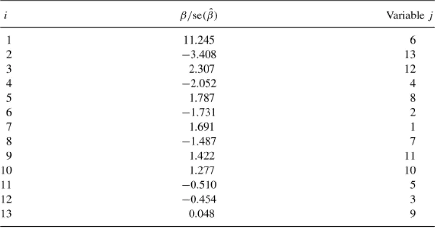
As an example of predictive performance, we report here some results of simulation based on the real data used in Johnson (1996). These data were originally taken to explore multiple regression to predict the percentage of body fat based on 13 predictors (body mea-surements) that are easily measured. We chose these data as a focus because they were used by Hoeting et al. (1999) in illustrating BIC and Bayesian model averaging (see also Burnham and Anderson 2002:268-84). The data are from a sample of 252 males, ages 21 to 81, and are available on the Web in conjunction with Johnson (1996). The Web site states, “The data were generously supplied by Dr. A. Garth Fisher, Human Performance Research Center, Brigham Young University, Provo, Utah 84602, who gave permission to freely distribute the data and use them for non-commercial purposes.”
We take the response variable asy = 1/D;Dis measured body density (observed minimum and maximum are 0.9950 and 1.1089, respectively). The correlations among the 13 predictors are strong but not extreme, are almost entirely positive, and range from−0.245 (age and height) to 0.941 (weight and hip circumference). The design matrix is full rank. The literature (e.g., Hoeting et al. 1999) supports that the measurements y and x = (x1, . . . , x13) on a subject can be suitably modeled as multivariate normal. Hence, we base simula-tion on a joint multivariate model mimicking these 14 variables by using the observed variance-covariance matrix as truth. From that full 14×14 observed variance-covariance matrix for y and x, as well as the theory of multivariate normal distributions, we computed
TABLE 1: Effects, asβ/se(βˆ), in the Models Used for Monte Carlo Simulation Based on the Body Fat Data to Get Predictive Mean Square Error Results by Model Selection Method (AICcor BIC) and Prediction Strategy (Best Model or Model Averaged) i β/se(β)ˆ Variablej 1 11.245 6 2 −3.408 13 3 2.307 12 4 −2.052 4 5 1.787 8 6 −1.731 2 7 1.691 1 8 −1.487 7 9 1.422 11 10 1.277 10 11 −0.510 5 12 −0.454 3 13 0.048 9
NOTE: Modelihas the effects listed on lines 1 toi, and its remainingβare 0. AIC=Akaike information criterion; BIC=Bayesian information criterion.
for the full linear model ofy, regressed onx, the theoretical regres-sion coefficients and their standard errors. The resultant theoretical effect sizes,βi/se(βˆi), taken as underlying the simulation, are given in Table 1, ordered from largest to smallest by their absolute values. Also shown is the index (j) of the actual predictor variable as ordered in Johnson (1996).
We generated data from 13 models that range from having only one huge effect size (generating Model 1) to the full tapering-effects model (Model 13). This was done by first generating a value of
x from its assumed 13-dimensional “marginal” multivariate distri-bution. Then we generated y = E(y|x) + ( was independent of x) for 13 specific models of Ei(y|x) with ∼normal (0, σi2),
i =1, . . . ,13. Given the generating structural model on expectedy,
σi was specified so that the total expected variation (structural plus residual) in y was always the same and was equal to the total vari-ation ofy in the original data. Thus, σ1, . . . , σ13 are monotonically decreasing.
For the structural data-generating models, we used E1(y|x) = β0 +β6x6 (generating Model 1), E2(y|x) = β0 +β6x6 +β13x13 (generating Model 2), and so forth. Without loss of generality, we
usedβ0=0. Thus, from Table 1, one can perceive the structure of each generating model reported on in Table 2. Theory asserts that under generating Model 1, BIC is relatively more preferred (leads to bet-ter predictions), but as the sequence of generating models progresses, K-L-based model selection becomes increasingly more preferred.
Independently from each generating model, we generated 10,000 samples of x andy, each of size n = 252. For each such sample, all possible 8,192 models were fit; that is, all-subsets model selec-tion was used based on all 13 predictor variables (regardless of the data-generating model). Model selection was then applied to this set of models using both AICc and BIC to find the corresponding sets of model weights (posterior model probabilities) and hence also the best model (with n =252, and maximumK being 15 AICc rather than AIC should be used). The full set of simulations took about two months of CPU time on a 1.9-GHz Pentium 4 computer.
The inference goal in this simulation was prediction. Therefore, after model fitting for each sample, we generated, from the same gen-erating model i, one additional statistically independent value ofx
and then ofE(y) ≡ Ei(y|x). Based on the fitted models from the generated sample data and this newx,E(y|x)was predicted (hence,
ˆ
E(y)), either from the selected best model or as the model-averaged prediction. The measure of prediction performance used was pre-dictive mean square error (PMSE), as given by the estimated (from 10,000 trials) expected value of(E(y)ˆ −Ei(y|x))2.
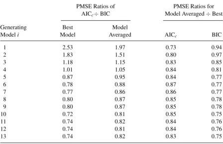
Thus, we obtained four PMSE values from each set of 10,000 trials: PMSE for both the “best” and “model-averaged” strategies for both AICcand BIC. Denote these as PMSE(AICc, best), PMSE(AICc, ma), PMSE(BIC, best), and PMSE(BIC, ma), respectively. Absolute values of these PMSEs are not of interest here because our goal is comparison of methods; hence, in Table 2, we report only ratios of these PMSEs. The first two columns of Table 2 compare results for AICc to those for BIC based on the ratios
PMSE(AICc,best)
PMSE(BIC,best) , column 1, Table 2
PMSE(AICc,ma)
TABLE 2: Ratios of Predictive Mean Square Error (PMSE) Based on Monte Carlo Simulation Patterned After the Body Fat Data, With 10,000 Independent Trials for Each Generating Model
PMSE Ratios of PMSE Ratios for AICc÷BIC Model Averaged÷Best
Generating Best Model
Modeli Model Averaged AICc BIC
1 2.53 1.97 0.73 0.94 2 1.83 1.51 0.80 0.97 3 1.18 1.15 0.83 0.85 4 1.01 1.05 0.84 0.81 5 0.87 0.95 0.84 0.77 6 0.78 0.88 0.87 0.77 7 0.77 0.86 0.86 0.77 8 0.80 0.87 0.85 0.78 9 0.80 0.87 0.85 0.78 10 0.72 0.81 0.85 0.75 11 0.74 0.82 0.84 0.76 12 0.74 0.81 0.84 0.76 13 0.74 0.82 0.83 0.75
NOTE: Margin of error for each ratio is 3 percent; generating modelihas exactlyieffects, ordered largest to smallest for Models 1 to 13 (see Table 1 and text for details). AIC=Akaike information criterion; BIC=Bayesian information criterion.
Thus, if AICc produces better prediction results for generating modeli, the value in that row for columns 1 or 2 is<1; otherwise, BIC is better.
The results are as qualitatively expected: Under a Figure 2 scenario with only a few big effects (or no effects), such as for generating Models 1 or 2, BIC outperforms AICc. But as we move more into a tapering-effects scenario (Figure 1), AICc is better. We also see from Table 2 that, by comparing columns 1 and 2, the performance difference of AICc versus BIC is reduced under model averaging: Column 2 values are generally closer to 1 than are column 1 values, under the same generating model.
Columns 3 and 4 of Table 2 compare the model-averaged to best-model strategy within AICcor BIC methods:
PMSE(AICc,ma) PMSE(AICc,best)
PMSE(BIC,ma)
PMSE(BIC,best), column 4, Table 2.
Thus, if model-averaged prediction is more accurate than best-model prediction, the value in column 3 or 4 is<1, which it always is. It is clear that here, for prediction, model averaging is always better than the best-model strategy. The literature and our own other research on this issue suggest that such a conclusion will hold generally. A final comment about information in Table 2, columns 3 and 4: The smaller the ratio, the more beneficial the model-averaging strategy compared to the best-model strategy.
In summary, we maintain that the proper way to compare AIC- and BIC-based model selection is in terms of achieved performance, espe-cially prediction but also confidence interval coverage. In so doing, it must be realized that these two criteria for computing model weights have their optimal performance under different conditions: AIC for tapering effects and BIC for when there are no effects at all or a few big effects and all others are zero effects (no intermediate effects, no tapering effects). Moreover, the extant evidence strongly supports that model averaging (where applicable) produces better performance for either AIC or BIC under all circumstances.
GOODNESS OF FIT AFTER MODEL SELECTION
Goodness-of-fit theory about the selected best model is a subject that has been almost totally ignored in the model selection litera-ture. In particular, if the global model fits the data, does the selected model also fit? This appears to be a virtually unexplored question; we have not seen it rigorously addressed in the statistical literature. Post–model selection fit is an issue deserving of attention; we present here some ideas and results on the issue. Full-blown simulation eval-uation would require a specific context of a data type and a class of models, data generation, model fitting, selection, and then application of an appropriate goodness-of-fit test (either absolute or at least rel-ative to the global model). This would be time-consuming, and one might wonder if the inferences would generalize to other contexts.
A simple, informative shortcut can be employed to gain insights into the relative fit of the selected best model compared to a global model assumed to fit the data. The key to this shortcut is to deal