FCND DISCUSSION PAPER NO. 184
Food Consumption and Nutrition Division International Food Policy Research Institute
2033 K Street, N.W. Washington, D.C. 20006 U.S.A.
(202) 862–5600 Fax: (202) 467–4439
July 2004
Copyright © 2004 International Food Policy Research Institute
FCND Discussion Papers contain preliminary material and research results, and are circulated prior to a full peer review in order to stimulate discussion and critical comment. It is expected that most Discussion Papers will eventually be published in some other form, and that their content may also be revised.
IMPACT EVALUATION OF A CONDITIONAL CASH
TRANSFER PROGRAM: THE NICARAGUAN
RED DE PROTECCIÓN SOCIAL
John A. Maluccio and Rafael FloresAbstract
This paper presents the main findings of a quantitative evaluation of the Red de Protección Social (RPS), a conditional cash transfer program in Nicaragua, against its primary objectives. These included supplementing income to increase household expenditures on food, reducing primary school desertion, and improving the health care and nutritional status of children under age 5. The evaluation design is based on a randomized, community-based intervention with measurements before and after the intervention in both treatment and control communities. Where possible, we erred on the side of assessing effects in conservative manners, for example, in the calculation of standard errors and the treatment of possible control group contamination. Overall, we find that RPS had positive (or favorable) and significant double-difference estimated average effects on a broad range of indicators and outcomes. Where it did not, it was often due to similar, smaller improvements in the control group that appear to have been stimulated indirectly by the program. Most of the estimated effects were larger for the extreme poor. The findings presented here played an important role in the decision to continue this effective program.
Contents
Acknowledgments... vii
1. Introduction... 1
2. Design and Implementation of the Red de Protección Social... 3
Program Targeting ... 3
Program Design ... 5
3. Design of the Evaluation and Methodology ... 12
Data Collection ... 13
Issues Related to the Experimental Design... 16
Double-Difference Methodology... 19
4. The Effects of Conditional Cash Transfers: The Red de Protección Social... 24
Household Expenditures ... 25
Schooling and Child Labor ... 36
Child Health Care ... 47
Growth Monitoring and Development Program Participation... 47
Vaccination for Children Ages 12–23 Months ... 51
Child Nutritional Status ... 53
5. Conclusions... 62
Appendix A: Household Targeting in Geographically Targeted Areas... 67
Appendix B: Table... 69
References... 70
Tables 1 Nicaraguan Red de Protección Social (RPS) eligibility and benefits in the pilot phase ... 8
2 Nicaraguan Red de Protección Social (RPS) beneficiary co-responsibilities monitored by Phase I ... 10
3 Nicaraguan Red de Protección Social (RPS) evaluation survey nonresponse
and subsequent attrition ... 16 4 Calculation of the double-difference estimate of average program effect... 20 5 Red de Protección Social (RPS) average effect on annual total household
expenditures ... 26 6 Red de Protección Social (RPS) average effect on per capita annual total
household expenditures... 29 7 Red de Protección Social (RPS) average effect on per capita annual food
expenditures ... 31 8 Red de Protección Social (RPS) average effect on food shares (percent)... 32 9 Red de Protección Social (RPS) average effect the composition of food
expenditures ... 34 10 Red de Protección Social (RPS) average effect on enrollment, children 7-to-13 years
old in first through fourth grades ... 40 11 Red de Protección Social (RPS) average effect on school advancement, children
7-to-13 years old in first through fourth grades (2000-2002), by starting grade ... 45 12 Red de Protección Social (RPS) average effect on school advancement, children
7-to-13 years old in first through fourth grades (2000-2002), by poverty group ... 45 13 Red de Protección Social (RPS) average effect on working, children 7-to-13
years old in first through fourth grades... 47 14 Red de Protección Social (RPS) average effect on percent of children age 0-3
taken to health control in past six months... 48 15 Red de Protección Social (RPS) average effect on percent of children age 0-3
taken to health control and weighed in past six months ... 49 16 Red de Protección Social (RPS) average effect on percent of children age 0-3
taken to health control and weighed in past six months, by poverty group... 50 17 Red de Protección Social (RPS) average effect on percent of children age 12-23
18 Malnutrition in Central American countries ... 56 19 Red de Protección Social (RPS) effect on percentage of children under 5 years
of age who are stunted (HAZ < -2.00)... 57 20 Red de Protección Social (RPS) effect on percentage of children under 5 years
of age who are wasted (WHZ < -2.00) ... 58 21 Red de Protección Social (RPS) effect on percentage of children under 5 years
of age who are underweight (WAZ < -2.00) ... 58 22 Red de Protección Social (RPS) effect on HAZ for children under 5 years of age.... 59 23 Red de Protección Social (RPS) average effect on percent of children ages 6-to-59
months given iron supplement (ferrous sulfate) in past four months ... 60 24 Red de Protección Social (RPS) effect on percentage of children 6-to-59 months
of age with anemia ... 61 25 Red de Protección Social (RPS) effect on average hemoglobin for children 6-to-59
months of age... 61
Appendix B Table
26 Indicators for (RPS) evaluation in Inter-American Development Bank
(IADB) loan contract ... 69
Figures
1 Illustration of the double-difference estimate of average program effect... 21 2 Density functions of per capita annual total expenditures in 2002: Control
versus intervention... 30 3a Enrollment in 2000 for 7-to-13-year-olds who have not completed fourth grade,
by age ... 37 3b Enrollment in 2000 for 7-to-13-year-olds who have not completed fourth grade,
4a Current attendance in 2000 for 7-to-13-year-olds who have not completed
fourth grade, by age ... 39 4b Current attendance in 2000 for 7-to-13-year-olds who have not completed
fourth grade, by expenditure group and by gender ... 39 5a Red de Protección Social (RPS) average effect on enrollment for
7-to-13-year-olds who have not completed fourth grade, by age ... 42 5b Red de Protección Social (RPS) average effect on enrollment for
7-to-13-year-olds who have not completed fourth grade, by expenditure group and by gender ... 42 6a Red de Protección Social (RPS) average effect on current attendance for
7-to-13-year-olds who have not completed fourth grade, by age ... 44 6b Red de Protección Social (RPS) average effect on current attendance for
7-to-13-year-olds who have not completed fourth grade, by expenditure group and by gender ... 44
Acknowledgments
This research began under the formal evaluation of the Nicaraguan Red de Protección Social by the International Food Policy Research Institute and in part draws from reports prepared under that project. We thank the Red de Protección Social team, particularly Tránsito Gómez, Caroll Herrera, and Mireille Vijil, for continued support during the evaluation. We thank Natàlia Caldés, Oscar Neidecker-Gonzalez, and Jane Rhode for research assistance, and David Coady, Alexis Murphy, Ferdinando Regalía, Marie Ruel, and Lisa Smith for many helpful comments.
John A. Maluccio
International Food Policy Research Institute Rafael Flores
Department of International Health Rollins School of Public Health Emory University
1. Introduction
In recent years, increasing emphasis has been placed on the importance of human capital in stimulating economic growth and social development. Consequently, investing in the human capital of the poor is widely seen as crucial to alleviating poverty,
particularly in the long term. There is also growing recognition of the need for social safety nets to protect poorer households from poverty and its consequences during the push for economic growth (World Bank 1997). While at first glance stimulating
economic growth and investing in social safety nets are apparently different strategies for economic development, both are important. They are also potentially complementary, as effective social safety nets may directly contribute to economic growth via improved human capital, particularly in the long term (Morley and Coady 2003).
Consistent with this view, several Latin American countries have introduced programs that integrate investing in human capital with access to a social safety net. One reason for the growing popularity of these programs is that by addressing various
dimensions of human capital, including nutritional status, health, and education, they are able to influence many of the key indicators highlighted in national poverty reduction strategies. One of the first, and largest, programs was the Programa Nacional de Educación, Salud y Alimentación (PROGRESA) in Mexico, begun in 1997. Another large program is the Programa de Asignación Familiar (PRAF) in Honduras. This paper examines a third, the Nicaraguan Red de Protección Social (RPS) or “Social Safety Net.”
The primary objective of these programs is to generate a sustained decrease in poverty in some of the most disadvantaged regions in their respective countries. Their basic premise is that a major cause of the intergenerational transmission of poverty is the inability of poor households to invest in the human capital of their children. Supply-side interventions, which increase the availability and quality of education and health services, are often ineffective in resolving this problem, since the resource constraints facing poor households preclude them from incurring the private costs associated with utilizing these services (e.g., travel costs and the opportunity cost of women’s and children’s time).
These programs attack this problem by targeting transfers to the poorest communities and households and conditioning the transfers on actions intended to improve children’s human capital development. This effectively transforms cash transfers into human capital subsidies for poor households.
Modeled after PROGRESA, RPS is designed to address both current and future poverty via cash transfers targeted to households living in poverty in rural Nicaragua. The transfers are conditional, and households are monitored to ensure that children are, among other things, attending school and making visits to preventive health-care providers. When households fail to fulfill those obligations, they lose their eligibility. By targeting the transfers to poor households, the program alleviates short-term poverty. By linking the transfers to investments in human capital, the program addresses long-run poverty. RPS’s specific objectives include
• supplementing household income for up to three years to increase expenditures on food,
• reducing school desertion during the first four years of primary school, and
• increasing the health care and nutritional status of children under age 5.
RPS comprised two phases over five years, starting in 2000. The pilot phase (also known as Phase I) lasted three years and had a budget of $11 million, representing
approximately 0.2 percent of GDP or 2 percent of annual recurring government spending on health and education (World Bank 2001, annex 21). As a condition of the Inter-American Development Bank (IADB) loan financing the project, and to assess whether the program merited expansion in the same or in an altered form, the Government of Nicaragua solicited various external evaluations of Phase I. The International Food Policy Research Institute (IFPRI) conducted the quantitative impact evaluation, using a randomized community-based design. In late 2002, based in part on the positive findings of the various evaluations, the Government of Nicaragua and IADB agreed to an
This paper presents the principal findings from the impact evaluation of RPS for a broad range of outcomes related to the program’s objectives, including (1) household (food) expenditures, (2) child schooling and child labor, (3) preventive health care of children under age 5, and (4) nutritional status of children under age 5. Though they are widely used and have a long history in developed countries, rigorous, large-scale, randomized evaluations of social programs such as the one reported on here remain rare in developing countries (National Research Council 2001; Newman, Rawlings, and Gertler 1994). Such studies have been increasing in popularity recently, however, after the widely cited case of PROGRESA (Skoufias 2003).
2. Design and Implementation of the Red de Protección Social
To analyze how a complex program like RPS altered behavior, it is first necessary to describe the program’s operation and evolution.
Program Targeting
In the design phase of RPS, rural areas in all 17 departments of Nicaragua were eligible for the program. The focus on rural areas reflects the distribution of poverty in Nicaragua—of the 48 percent of Nicaraguans designated as poor in 1998, 75 percent resided in rural areas. For the pilot, the Government of Nicaragua selected the
departments of Madriz and Matagalpa from the northern part of the Central Region, on the basis of poverty as well as on their capacity to implement the program. This region was the only one that showed worsening poverty between 1998 and 2001, a period during which both urban and rural poverty rates declined nationally (World Bank 2003). In 1998, approximately 80 percent of the rural population of Madriz and Matagalpa were poor, and half of those were extremely poor (IFPRI 2002). In addition, these departments had easy physical access and communication (including being less than a one-day drive from the capital, Managua, where RPS is headquartered), relatively strong institutional capacity and local coordination, and reasonably good coverage of health posts and
schools (Arcia 1999). By purposively targeting, RPS avoided devoting a
disproportionate share of its resources during the pilot to increasing the supply of educational and health services.
In the next stage of geographic targeting, all six (out of 20) municipalities that had the participatory development program Microplanificación Participativa (Participatory Micro-planning), run by the national Fondo de Inversión Social de Emergencia (FISE), were chosen.1 The goal of that program was to develop the capacity of municipal governments to select, implement, and monitor social infrastructure projects such as school and health post construction, with an emphasis on local participation. It is possible, then, that the selected municipalities had atypical capacity to carry out RPS. Nevertheless, in terms of poverty, the six municipalities were well targeted. Between 36 and 61 percent of the rural population in each of the chosen municipalities were
extremely poor and between 78 and 90 percent were extremely poor or poor (IFPRI 2002), compared with national averages of 21 and 45 percent, respectively (World Bank 2003). While not the poorest municipalities in the country (or in the chosen departments for that matter), the proportion of impoverished people living in these areas was still well above the national average.
In the last stage of geographic targeting, a marginality index based on information from the 1995 National Population and Housing Census was constructed, and an index score was calculated for all 59 rural census comarcas2 in the selected municipalities. The index was a weighted average of the following set of poverty indicators (with respective weights in parentheses) known to be highly associated with poverty (Arcia 1999):
1. family size (10 percent),
2. access to potable water (50 percent),
1 The six were Totogalpa and Yalagüina municipalities in the department of Madriz, and Terrabona,
Esquipulas, El Tuma-La Dalia, and Ciudad Darío municipalities in the department of Matagalpa.
2 Comarcas are administrative areas within municipalities that include between one and five small communities averaging 100 households each.
3. access to latrines (30 percent), and 4. illiteracy rates (10 percent).
Higher index scores were associated with more impoverished areas. Recognizing that the index could not reliably distinguish between two comarcas with similar scores, rather than use the scores directly, the 59 rural comarcas were grouped into four priority levels after renormalizing the highest index score to 100: a score of above 85 was given highest priority (priority 1); 70–85, priority 2; 60–70, priority 3; and below 60, lowest priority, 4.3 The 42 comarcas with the priority scores 1 and 2 were eligible for the pilot phase’s first stage.
Program Design
RPS has two core components:
1. Food security, health, and nutrition. Each eligible household receives a cash transfer known as the bono alimentario or “food security transfer,”4 every other month, contingent on attendance at educational workshops held every other month and on bringing their children under age 5 for scheduled preventive (or well child) health-care appointments. The workshops are held within the
communities and typically include about 20 participants. They educate women in household sanitation and hygiene, nutrition, reproductive health, breastfeeding, and related topics.
To ensure adequate supply, RPS trained and paid private providers to deliver the specific health-care services required by the program. These services, provided free of charge to beneficiary households, include growth and
3 IFPRI (2002) describes RPS targeting in more detail.
4 One common definition of food security is “when all people at all times have both the physical and
economic access sufficient to meet their dietary needs in order to lead a healthy and productive life” (USAID 1992). In this paper, we do not formally assess food security, however, but focus on indicators of food expenditures that are associated with food security.
development monitoring, vaccination, and provision of antiparasites, vitamins, and iron supplements. Children under age 2 are seen monthly and those between 2 and 5, every other month. In practice, mothers bring their children to the local service location (often a community center or house of one of the beneficiaries) to be seen by the doctor working for the private provider. First, the professional nurse measures the child, inquires about the child’s health and the caretaker’s caring and feeding practices, and checks the vitamin A supplementation record. Then the doctor examines the child, prescribing appropriate antiparasite medicine or iron supplements according to the Ministry of Health protocol for making these prescriptions. If the child is growing well, the doctor congratulates the caretaker. Then the caretaker returns to the nurse to receive individual counselingon how to maintain or improve growth with key messages on breastfeeding, child feeding, illness care, and hygiene, taking into account several factors, such as the age of the child and whether the child gained weight adequately the previous month or had been ill. The RPS adapted the individual counseling material from the
Atención Integral a la Niñez (Integrated Attention to the Child, or AIN) program in Honduras (Van Roekel et al. 2002).
2. Education. Each eligible household receives a cash transfer known as the bono escolar or “school attendance transfer” every other month, contingent on
enrollment and regular school attendance of children ages 7–13 who have not completed fourth grade of primary school. Additionally, for each eligible child, the household receives an annual cash transfer intended for school supplies (including uniforms and shoes) known as the mochila escolar or “school supplies transfer,” which is contingent on enrollment. Unlike the school attendance transfer, which is a fixed amount per household regardless of the number of children in school, the school supplies transfer is for each child.
To provide incentives to the teachers, who have some additional reporting duties and were likely to have larger classes after the introduction of RPS, and to
increase resources available to the schools, there is also a small cash transfer, known as the bono a la oferta or “teacher transfer.”5 This is given to each beneficiary child, who in turn delivers it to the teacher. The teacher keeps one-half, while the other half is earmarked for the school. The delivery of the funds to the teacher is monitored, but not their ultimate use.
Table 1 summarizes the eligibility requirements and demand and supply-side benefits of RPS. At the outset, nearly all households were eligible for the food security transfer, which is a fixed amount per household, regardless of household size (Appendix A describes the small number of households that were not eligible). Households with children ages 7–13 who had not yet completed the fourth grade of primary school were also eligible for the education component of the program.
The amounts for each transfer were initially determined in U.S. dollars and then converted into Nicaraguan córdobas (C$) in September 2000, just before RPS began distribution. Table 1 shows the original U.S. dollar annual amounts and their Nicaraguan córdoba equivalents (using the September [2003] average exchange rate of C$12.85 to US$1). The food security transfer was $224 a year, and the school attendance transfer $112.6 On its own, the food security transfer represents about 13 percent of total annual household expenditures in beneficiary households before the program. A household with one child benefiting from the education component would receive additional transfers of
5 In rural Nicaragua, school’s parents’ associations often request small monthly contributions from parents
to support the teacher and the school; the teacher transfer was, in part, intended to supplant those informal fees.
6 The calculations for the transfer amounts were based on the extreme poverty gap, i.e., the difference
between the extreme poverty line and the average level of expenditures of the extreme poor reported in the 1998 LSMS (World Bank 2001). The 1998 daily per capita extreme poverty line (calculated to enable the purchase of a minimum requirement food basket) is $0.58 and the extreme poverty gap, $0.18. For comparison, the 1998 daily per capita poverty line is $1.12. The amount for the school attendance transfer was calculated using an approximation of the opportunity cost of children multiplied by the average number of children ages 7–13 in households in extreme poverty. The sum of the food and school attendance transfers was an estimated average daily transfer of $0.12, an amount that would fill two-thirds of the average extreme poverty gap for extremely poor households.
Table 1—Nicaraguan Red de Protección Social (RPS) eligibility and benefits in the pilot phase
Program components
Food security, health, and nutrition Education ELIGIBILITY
Geographic targeting All householdsa All householdsa with children ages 7-13
who have not yet completed fourth grade of primary school
DEMAND-SIDE BENEFITS
Monetary transfers Bono alimentario
(food security transfer) (school attendance transfer)Bono escolar
CS2,880 per household per year (US$224) C$1,440 per household per year (US$112)
Mochila escolar (school supplies transfer)
C$275 per child beginning of school year (US$21)
SUPPLY-SIDE BENEFITS Services provided and
monetary transfers
Bimonthly health education workshops Child growth and monitoring
-Monthly (0-2 year olds)
-Bimonthly (2-5 year olds) (teacher transfer)Bono a la oferta
(C$60 per child per year given to teacher/school (US$5) Provision of antiparasites, vitamins, and
iron supplements Vaccinations (0-5 year olds)
a As described in Appendix A, a small percentage of households were excluded.
about 8 percent, yielding an average total potential transfer of 21 percent of total annual household expenditures. Over the two years, the actual average monetary transfer
(excluding the teacher transfer) was approximately C$3,800 (or 18 percent of total annual household expenditures). This is approximately the same percentage of total annual household expenditures as the average transfer in PROGRESA, but more than five times as large as the transfers given in PRAF. In contrast to PROGRESA, which indexes transfers to inflation, the nominal value of the transfers remained constant for RPS, with the consequence that the real value of the transfers declined by about 8 percent over two years in the pilot phase due to inflation. It is possible that any differences in the
effectiveness of RPS between 2001 and 2002 resulted, in part, from a decline in the real value of the transfers, though such effects are likely to be small.
The value of the supply-side services, as measured by how much RPS paid to the providers, was also substantial. On an annual basis, the education workshops cost
approximately $50 per beneficiary and the health services for children under age 5, approximately $110, including the value of the vaccines, antiparasites, vitamins, and iron supplements, all of which were provided by the Ministry of Health.
To enforce compliance with program requirements, beneficiaries did not receive the food or education component of the transfer if they failed to carry out any of the conditions listed in Table 2. The monitoring is done using the management information system (MIS) designed specifically for and by RPS. It comprises a continuously updated, relational database of beneficiaries, health-care providers, and schools. The MIS is also used to (1) select beneficiaries and prepare invitations to program incorporation
assemblies, (2) calculate transfer payments, (3) compile requests to the Ministry of Health for vaccines and other materials, and (4) monitor whether service providers are meeting their responsibilities. Decision rules capturing the requirements in Table 2 are programmed directly into the MIS. Substantial time was dedicated to designing data forms for the various program participants that feed into this system (including the household registry or census forms, school forms, and health-care provider forms that are all sent to the main office where they are entered into the computer).
Table 2 shows the four different “types” of beneficiary households in the program, who receive different transfers and have to fulfill different requirements. Households with no children in the targeted age ranges are only eligible for the food security transfer but, at the same time, need only attend the health education workshops to qualify for continued receipt of the transfers. Households with children under age 5 (but without children ages 7–13 who have not completed the fourth grade) are also
eligible for the food security transfer only, but have more requirements to fulfill related to their young children. Households with children ages 7–13 who have not completed the fourth grade are eligible for both the food security and education transfers and are required to comply with the school-related conditions. If, in addition, there are children under age 5 in the household, it is eligible for the same transfers, but has more
requirements to fulfill, in particular, those related to the health controls for young children.
Table 2—Nicaraguan Red de Protección Social (RPS) beneficiary co-responsibilities monitored by Phase I Household type Program requirement Households with no targeted children (A) Households with children ages 0-5 (B) Households with children ages 7-13 who
have not completed fourth grade
(C) (B) + (C) Attend bimonthly health education workshops ! ! ! ! Bring children to prescheduled health-care
appointments
Monthly (0-2 years) ! !
Every other month (2-5 years)
Adequate weight gain for children under 5a ! !
Enrollment in Grades 1 to 4 of all targeted children
in the household ! !
Regular attendance (85 percent), i.e., no more than five absences every two months without valid
excuse) of all targeted children in the household ! ! Promotion at end of school yearb ! !
Deliver teacher transfer to teacher ! ! Up-to-date vaccination for all children under 5
yearsb ! !
a The adequate weight gain requirement was discontinued in Phase II starting in 2003. b Condition was not enforced
RPS allows this latter type of household to receive a partial transfer if it complies with the health-care requirements and not the education requirements or vice versa. During the first two years of transfers, approximately 10 percent of beneficiaries were penalized at least once and therefore did not receive, or received only part of, their transfer. It was also possible for households to be expelled from the program.7 At the start of the program, about 90 percent of the households in the intervention areas were participating (see Appendix A). Less than 1 percent of households were expelled during the first two years of delivering transfers, though 5 percent voluntarily left the program, e.g., by dropping out or migrating out of the program area.
7 Causes for expulsion include (1) repeated failure to comply with program requirements, (2) failure to
collect the transfer in two consecutive pay periods, (3) more than 27 unexcused school absences during the school year per beneficiary child, (4) failure of a beneficiary child to be promoted to the next grade, and (5) discovery of false reporting of information during any part of data collection, including information about fulfillment of program responsibilities.
When it was learned that some, but not all, schools practiced automatic promotion, enforcement of the grade promotion condition was deemed unfair and
therefore was never enforced. Similarly, when there were some delays in the delivery of vaccines, the up-to-date vaccination condition was also deemed unfair and not enforced. A third condition, punishment of children who did not have adequate weight gain, was dropped at the end of the pilot phase because of a concern about the role of measurement error and the finding that the poorest households were more likely to be punished. These changes highlight the importance of careful consideration of the required responsibilities and how they are to be monitored during the design of a conditional cash transfer
program. At the same time, they show the importance of flexibility during program implementation.
Only the designated household representativecould collect the cash transfers and, where possible, RPS designated the mother as the household representative. This
strategy mimics the design of PROGRESA and PRAF and is based on evidence that resources in the hands of women often lead to better outcomes for child well-being and household food security (Strauss and Thomas 1995). As a result, more than 95 percent of the household representatives were women. These representatives attended the health education workshops and they were responsible for ensuring that the requirements for their households were fulfilled. In a small number of multigenerational households, the grandmother was selected as the household representative. Since the workshops at times cover themes such as family planning, flexibility on who attends the sessions might be called for in this area.
Although centrally administered, with its multisectoral approach across education, health, and nutrition, RPS required bureaucratic cooperation at national, municipal, and community levels. Given funding and administrative oversight from FISE, municipal planning and coordination was conducted by committees composed of delegates from the health and education ministries, representatives from civil society, and RPS personnel. This coordination proved important in directing supply-side responses to increased household demand for health and schooling services. At the comarca level, RPS
representatives worked with local volunteer representatives known as promotoras
(beneficiary women chosen by the community) and local school and health-care service providers, to implement the program. The promotoras were charged with keeping beneficiary household representatives informed about upcoming health-care
appointments for their children, upcoming payments, and any failures in fulfilling the conditions. Each promotora had, on average, 17 beneficiaries in her charge, though this average masked substantial variation ranging from 5 to 30 beneficiaries.
3. Design of the Evaluation and Methodology
The evaluation design is based on a randomized, community-based intervention with measurements before and after the intervention in both treatment and control communities. One-half of the 42 comarcas (targeted in the first stage as described in the first portion of Section 2) were randomly selected into the program. Thus, there are 21
comarcas in the intervention group and 21 in the control group (IFPRI 2001a). Including a control was ethical because the effectiveness of the intervention was unknown. In addition, there was not sufficient capacity to implement the intervention everywhere. Given the geography of the program area, control and intervention comarcas are at times adjacent to one another. The selection was done at a public event with representatives from the comarcas, the Government of Nicaragua, IADB, IFPRI, and the media present. The 42 comarcas were ordered by their marginality index scores and stratified into seven groups of six each. Within each stratum, randomization was achieved by blindly drawing one of six colored balls (three blue for intervention, three white for control) from a box after the name of each comarca was called out. Thus, three comarcas from each group were randomly selected for inclusion in the program, while the other three were selected as controls.
The evaluation was designed to last for one year; that is, the control group was meant to be a control for only one year (after which it was expected there would be capacity to implement the intervention everywhere). Due to delays in funding for RPS as
a result of a governmental audit unrelated to the program, however, incorporation of beneficiaries in the control comarcas was postponed until 2003, extending the possible length of the treatment-control evaluation by more than a year. In fact, control comarcas
waited a little over two years before being fully incorporated into the program.
Data Collection
The data collected for the evaluation are from an annual household panel data survey implemented in both intervention and control areas of RPS before the start of the program in 2000, and in 2001 and 2002 after the program began operations.8 The questionnaire was a comprehensive household questionnaire based on the 1998
Nicaraguan LSMS instrument, expanded in some areas (e.g., child health and education) to ensure that all the necessary program indicators were captured, but cut in other areas (e.g., income from labor and other sources) to minimize respondent burden and ensure collection of high-quality data in a single interview.9 An anthropometric module for children under age 5 was implemented in 200010 and 2002, but not in 2001. In this module, we measured height (or length) and weight; we also measured hemoglobin using portable (Hemocue) machines and following standard international procedures.
The survey sample is a stratified random-sample at the comarca level from all 42
comarcas described above. The areas represented comprise a relatively poor part of the rural Central Region in Nicaragua, but the sample is not statistically representative of the six municipalities (or other areas of Nicaragua, for that matter). Forty-two households were randomly selected in each comarca using a census carried out by RPS three months prior to the survey as the sample frame, yielding an initial target sample of 1,764
households. The sample size calculation was based on assessing the necessary sample sizes for the indicators listed in Appendix B, Table 26. Assuming a random sample, the
8 Results reported on here are based on the September 2003 release of the RPS evaluation data.
9 LSMS surveys are typically implemented in two visits to the household (Grosh and Glewwe 2000).
10 About one-half of the 2000 anthropometry survey had to be completed in early October, one month after
indicator that required the largest sample size, using a significance level of 5 percent and a power of 80 percent, was enrollment for Grades 1–4 (indicator 5 in Appendix B, Table 26). To detect a minimum, statistically significant difference of eight percentage points between intervention and control groups, a sample size of 549 students for each group was required. Of course, not all households had children in this age group. According to the 2000 RPS population census, 63 percent of households had at least one child between ages 6 and 12. Therefore, to obtain a sample of 549 children (in different households), it was necessary to interview 871 households in each group (549 ÷ 0.63) or 1,742 in total. Thus, we arrived at a target sample of 1,764 households.11 The first wave of fieldwork was carried out in late August and early September 2000, without replacement—that is, when it was not possible to interview a selected household, another household was not substituted.
While there was a great deal of progress in getting RPS started throughout 2001, it was not possible to design and implement all the components according to the original timelines. In particular, the health-care component was not initiated until June 2001. This delay occurred because it took longer than originally planned to design the intervention and select, contract, and train the NGO and private health-care providers. There were also delays in the payment of transfers to households due to a governmental audit that effectively froze RPS funds. As a result, the RPS 2001 follow-up survey was delayed until the beginning of October, to allow additional time for the interventions to take root and for five of the scheduled six payments to be effected. Of course, the advantage of the original design, with the scheduled RPS follow-up at exactly the same time of year as in the 2000 baseline, was that it would enable us to control better for possible seasonal variations in consumption and health. With a control group, however, the possible bias introduced by seasonality can be controlled for statistically. This difference in the timing of the survey, then, does not present a serious problem for the
11 IFPRI (2001a) describes the sample size calculations in more detail and IFPRI (2001b and 2003) describe
the baseline and follow-up samples in more detail. Since anthropometric measures were not part of the original indicator list to be evaluated, they were not used in sample size calculations.
estimation of average effects of the program. The delay in the survey work had the advantage of giving the program more time to take effect, thereby providing a more realistic evaluation of program operations (rather than an evaluation of program delays). In October 2001, then, beneficiaries had been receiving transfers, and the educational components of the program had been monitored for 13 months, but they had only received five months of the health and nutrition services, including the health education workshops. This unforeseen change in operations illustrates the importance of having a credible control group—without the control, it would have been very risky to change the timing of the survey and still confidently attribute observed changes to RPS. The 2002 survey was also carried out in October, and in the second year, beneficiaries received all components of the program for a full 12 months.
We now document nonresponse in the 2000 baseline survey and attrition in the follow-up surveys. Overall, 90 percent (1,581) of the stratified random sample was interviewed in the first round (see Table 3). In a handful of comarcas, the coverage was 100 percent, but in six, it was under 80 percent. For the follow-up surveys in October 2001 and October 2002, the target sample was limited to these 1,581 first-round interviews. In 2002, just over 90 percent of these were reinterviewed, on a par with surveys of similar magnitude in other developing countries (Alderman et al. 2001; Thomas, Frankenberg, and Smith 2001). Again, however, coverage in six of the
comarcas was substantially worse, with less than 80 percent successfully reinterviewed (and one of these is one of the six from above with high first-round nonresponse rate). This attrition is unlikely to have been random (a theme we return to later). Because the same target sample was used in 2002 as in 2001, regardless of whether the household was interviewed in 2001, some households that were not interviewed in 2001 were
successfully interviewed in 2002. The sample for which there is a complete set of observations (one in each of the three survey rounds) is 1,396, smaller than the 1,434 shown in the first row of the third column of Table 3. The households are about evenly divided between intervention and control groups, indicating that at least the level of attrition was not significantly different between them.
Table 3—Nicaraguan Red de Protección Social (RPS) evaluation survey nonresponse and subsequent attrition
Baseline 2000 Follow-up 2001 Follow-up 2002
Completed interview 1,581 1,490 1,434
(89.6) (94.2) (90.7)
Completed interview in all three rounds 1,396 1,396 1,396
(79.1) (88.3) (88.3) ...of which Intervention 706 706 706 (percent intervention) (80.0) (87.2) (87.2) Control 690 690 690 (percent control) (78.2) (89.5) (89.5) Not interviewed Uninhabited dwelling 60 51 83 Temporary absence 100 28 46 Refusal 16 6 12 Urban (misclassified) 6 0 0 Lost questionnaire 0 6 6 Target sample 1,764 1,581 1,581
Note: Percent of target sample in parentheses.
Issues Related to the Experimental Design
To measure program impact, it is necessary to know what would have happened had the program not been implemented. The fundamental problem, of course, is that an individual, household, or geographic area cannot simultaneously undergo and not
undergo an intervention. Therefore, it is necessary to construct a counterfactual measure of what might have happened had the program not been available. The most powerful way to construct a valid counterfactual is to randomly select beneficiaries from a pool of equally eligible candidates. This was done for the evaluation of RPS using a community-based randomized intervention (IFPRI 2001a).
The value of such randomized evaluations is widely recognized. When done well, recipients and nonrecipients will have, on average, the same observed and, more
important (since they are more difficult to control for), unobserved characteristics. As a result, they establish a credible basis for comparison, freed from selectivity concerns, and the direction of causality is certain. Nonrandomized approaches, on the other hand, typically rely on assumptions that are often hard to believe and almost always hard to
verify (Burtless 1995). A further advantage to a randomized design is that program impact is easy to calculate and, as a consequence, easier to understand and explain.12
However, even a well-implemented randomized evaluation design is not without its weaknesses. First, the usual difficulties of following subjects over time persist, so selection bias due to attrition remains a potential problem; the advantages of
randomization are dissipated with attrition if it is nonrandom. Second, such studies can be costly (financially and politically), and often one must wait years for results, making them less useful for making pressing policy decisions. Third, there are important ethical concerns about withholding treatment from the control group of an intervention known to have positive effects. In RPS, the randomized design was justified because it had not been shown to have positive effects and because of the infeasibility, given the fixed budget, of extending the program to all potential beneficiaries in a short period of time. In this case, random selection would appear to be as fair as any other arbitrary criterion for selecting the first set of beneficiaries.
Unfortunately, randomized design evaluations can provide only partial answers to important questions they are not explicitly designed to address. This is often referred to as their “black box” nature. The evaluation only allows us to assess the effect of the program (or program components) it was explicitly designed to assess. In the case of the RPS evaluation, this means that we only evaluate the program as a whole, with all of its components. Without further assumptions, we are in the dark if we want to consider how even slightly changing the program would alter the outcomes under consideration. For example, RPS provides a “package” of services in which all households are eligible for the food security transfer, regardless of whether they also receive the educational
transfers. With only the randomized design implemented here, it is not possible to isolate
12 Heckman and Smith (1995), however, point out that this apparent simplicity can be deceiving,
particularly in poorly designed evaluations where there is randomization bias (where the process of randomization itself leads to a different beneficiary pool than would otherwise have been treated) or substitution bias where nonbeneficiaries obtain similar treatments from different sources—a form of “contamination.” The former should not be a concern in the RPS evaluation. We discuss the reasons for this later.
the effects of just the educational transfer—all the observed effects are the result of the program as a whole. Nor is it possible, without further assumptions, to assess reliably what the effect of the program would be if the size of the transfers were to change, as they did when expansion of the program began in 2003.
Another limitation of randomized evaluations is that the results pertain
specifically to the study population—extrapolating them to other populations requires additional assumptions that may not be easy to verify (Burtless 1995). This is typically referred to as the external validity problem. In the case of RPS, the purposive selection of program areas may have affected program performance; therefore the generalizability of the results is questionable. As described earlier, the selection of municipalities was conditioned on the likelihood of success, so that the observed outcomes might exaggerate the likely outcomes from program expansion to other areas with, for example, weaker institutional capacity to implement the program.
A final problem to bear in mind when interpreting the results in this analysis is that the program was in its pilot phase, and outcomes (and therefore estimated effects) for the pilot may differ from outcomes for an expanded program. Like most pilots, RPS underwent an initial learning period (with attendant setbacks) and undertook a variety of activities that might not need repeating in an expansion (e.g., preparing training materials for beneficiaries, promotoras, and health-care providers). Some of these activities could have reduced the program’s effectiveness during the pilot (Caldés and Maluccio 2004). Moreover, as with any new program, there was the potential for observed behavioral changes to result, in part from the novelty of the program or the evaluation rather than from permanent behavioral changes—the Hawthorne effect (Krueger 1999). There is some evidence consistent with this phenomenon when we compare the effects after one year (2000–01) with those after two years (2000–02). Performance was slightly lower in 2002 than in 2001 on several outcome indicators. Unfortunately, we cannot directly test whether this is due to a Hawthorne effect, changes in the effectiveness of program implementation, or the slight decline in the real value of transfers. Finally, expansion of the program could introduce new advantages and disadvantages associated with scaling
up and economies of scale. All these factors call for a degree of caution in forecasting what would happen were the program to be extended to other municipalities or
departments of Nicaragua.
Double-Difference Methodology
Household- and individual-level data were collected in both the intervention and control comarcas before and after RPS was implemented. This enables the use of the double-difference method to calculate “average program impact.”13 The resulting measures can be interpreted as the expected effect of implementing the program in a similar population elsewhere, subject to the caveats discussed above. The method is shown in Table 4. The columns distinguish between groups with and without the
program (denoted by I for intervention and C for control), and the rows distinguish before and after the program (denoted by subscripts 0 and 1). Anticipating one of the analyses presented below, consider the measurement of school enrollment rates for children. Before the program, we would expect the average percentage enrolled to be similar for the two groups, so that the quantity (I0 – C0) would be close to zero. After the program has been implemented, however, we would expect differences between the groups as a result of the program. Furthermore, because of the random assignment, we expect the difference (I1 – C1) to measure the effect directly attributable to the program. Indeed, (I1 – C1) is a valid measure of the average program effect under this design and is referred to as the first difference. A more robust measure of the effect, however, would account for any preexisting observable or unobservable differences between the two randomly assigned groups: this is the double difference obtained by subtracting the preexisting differences between the groups, (I0 – C0), from the difference after the program has been implemented, (I1 – C1).
Table 4—Calculation of the double-difference estimate of average program effect
Survey round Intervention group with RPS program without RPS program Control group Difference across groups
Follow-up I1 C1 I1 – C1
Baseline I0 C0 I0 – C0
Difference across time I1 – I0 C1 – C0 (Double-difference I
1 – C1) – (I0 – C0)
An alternative interpretation of the double-difference estimator emerges if one first considers the differences within the (intervention or control) groups. This approach begins with a naive estimator of the program effect, the difference over time for the intervention group, (I1 - I0).14 It is naive because it would include all changes over time in enrollment rates in the intervention group, regardless of what causes them. For example, if increases in public investment nationally were improving school access and leading to changes in enrollment, these effects would show up in the difference over time in the intervention group, in addition to the effects attributable to the program. The obvious measure for the nonprogram-related change over time in the intervention group is the change over time in the control group, (C1 - C0). Thus we estimate the average program effect by first considering the total change over time in the intervention group, and then subtracting from this the change over time in the control group. As above, this yields the double-difference estimator.
The alternative interpretation is probably best illustrated graphically in Figure 1. For an arbitrary indicator that we measure over time, we assume (for the graph) that as a result of the randomization, both the intervention and control groups start at the same level. No change in the indicator over time would lead to the outcome depicted by point A in 2002; if we were only following the intervention group, we would then naively calculate the effect of the program as C - A. However, as the control group makes clear,
there was a trend over time that led to an improvement (in this example) of B - A. Were we to ignore this, we would overstate the effect of the program. Instead, our estimate of the program effect is C - B; this is the double difference estimate. In the case where the trend line for the control group was declining, ignoring that effect would tend to
understate the program effect.15
Figure 1—Illustration of the double-difference estimate of average program effect
Baseline Follow-up
For this work, the technique just described is extended to account for the three measurements taken in 2000, 2001, and 2002. The basic estimating equation is
Eict = α0 + α1 A1 + α2 A2 + α3 Pc + δ1A1 Pc + δ2 A2 Pc + µic + νict, (1) where
Eict = outcome variable of interest for household (or individual) i in comarcac
at time t,
A1 = (1) if Year 2001,
A2 = (1) if Year 2002,
15 Relaxing the (unnecessary) assumption that the two groups start at identical points slightly complicates
the graphical exposition, but the logic remains the same. Control Intervention
A B C
Pc = (1) if program intervention in comarca c,
µic = all (observed and unobserved) household- (or individual-) level time-invariant factors,
νict = unobserved idiosyncratic household (or individual) and time-varying error, and
all the α and δ are unknown parameters.
The parameters of interest are δ1 and δ2; δ1 is the double-difference estimator of the average program effect for 2001 (relative to 2000), and δ2 for 2002 (relative to 2000). We emphasize that the program effects are identified by the randomized design; given the randomization of Pc, it (and any interactions involving it) is uncorrelated with all
observed or unobserved household- (or comarca-) level variables so that the δs can be consistently estimated. Indeed, the main reason to include household variables in a regression like this is to increase the precision of the estimates, not because we are concerned about the consistency of the estimator for δ. As a robustness check on the results (described later), we include household-level effects and find no substantive differences in the estimates of the program effects, other than that they tend to be much more highly significant.16
To assess differences in effects for the poor and nonpoor for all the analyses considered below, we also classify households into three poverty groups—extreme poor, poor, and nonpoor—based on their per capita annual total household expenditures (including own-production) measured in 2000 and using 2001 national poverty lines developed by the World Bank (World Bank 2003).17 Double-difference estimates were
16 Due to the random allocation of the program, none of the explanatory variables in equation (1) would be
correlated with household-level effects, so we can safely treat them as either random or fixed. The results are similar for the two different approaches.
17 Another approach we considered for calculating the poverty groups was to adjust the 1998 national
poverty lines for inflation up to 2000. That methodology yields poverty lines that are similar but 3–4 percent higher than the 2001 national lines, since general inflation tends to outpace increases in the poverty line, given the more limited consumption basket on which the latter is based. Categorizations based on this alternative approach do not substantively change the reported results.
calculated within each poverty group and are discussed in the text (and presented in some of the tables) when they differ across the groups.
Finally, since we do not condition on the individual household-level decision to participate but instead only on whether the program was available in the household’s
comarca, we are estimating what is commonly referred to as the “intent to treat” effect. Recall that about 10 percent of the households in the intervention areas were either excluded by RPS or chose not to participate. Survey sample households in this subgroup are not program beneficiaries, so basing estimates that combine them with beneficiary households dilutes the estimated effects of the program. The intent-to-treat methodology is a conservative one relative to measuring the effect of the treatment on the treated, though given the relatively high participation rates; it is unlikely to underestimate the effect on participating households by much. Furthermore, the intent-to-treat estimate is less subject to selection biases associated with the decision to participate in the program. Finally, the advantages of the randomized design are dissipated if we estimate the effect of the treatment on the treated, since the evaluation was not designed to do that. Rather than estimating the double difference, we would instead have to endogenize the
participation decision, most likely by using the random program placement as an instrumental variable.
In the double-difference analyses that follow, all (relevant) individuals or
households from each survey round, regardless of whether they were interviewed in one, two, or three of the waves, are included. On the whole, there were few significant differences between households (or individuals) in intervention and control groups at baseline; even when there were, of course, the double-difference estimator controls for them. All standard errors are calculated allowing for heteroscedasticity and for clustering at the comarca level (Stata Corporation 2001). We do not control for the fact that the randomization was at the comarca level—so-called “community effects.” When we do not control for heteroscedasticity and comarca-level clustering, or when we do control for community-level effects, the standard errors decrease, leading to stronger statistical
significance. Consequently, the results we present are conservative in terms of their significance.
We also ignore the stratified sample design, which can be corrected for statistically by using comarca-level sample weights; correcting for this aspect of the design made no substantive changes to the estimated effects, so we chose not to do so in order to present estimates with the more conservatively estimated standard errors
described above. Similarly, when we limit the sample to those interviewed in all three rounds as a partial control for attrition bias, estimated effects change only slightly, with no systematic bias.
Another partial remedy to control for attrition bias is to estimate a household fixed-effects model, particularly if one suspects that unobserved persistent heterogeneity is leading to attrition. However, as with the other robustness checks, when we estimate the models with these controls, the results differ little. Recall that the number of
households is about evenly divided between intervention and control groups, suggesting that attrition was not significantly different between intervention and control groups. Combining this with the evidence from the robustness checks just described, we conclude that attrition bias is not driving the results presented here.
4. The Effects of Conditional Cash Transfers: The Red de Protección Social
As a condition for approval of the second tranche of the IADB loan underwriting RPS, an evaluation was carried out by IFPRI assessing the main objectives of the
program. The IADB loan document contained a set of specific indicators and numerical goals for each objective (see Appendix B, Table 26), and these were used in the sample size calculations described in the first portion of Section 3. While the program achieved most of these goals and the loan extension was approved, we do not emphasize these specific indicators in our analysis. This is because (1) they represent only a subset of the possible effects of the program, (2) at the time, the program designers had little
and (3) they largely measure process or inputs and did not capture the underlying
objectives of the program such as improved human capital. While we are in favor of the trend by development institutions to embed project evaluations in projects, we would caution against overspecifying the goals or holding to them too rigidly, particularly when little evidence of similar programs exists. Hence, while we present results for the
contractually agreed-to indicators, we do not compare the results with the numerical goals. Moreover, we present results on a large number of additional indicators including direct measures of one form of human capital, the nutritional status of children under age 5.
Household Expenditures
At the outset, we indicated that 36–61 percent of the rural population in each of the RPS municipalities was extremely poor, and 78–90 percent was extremely poor or poor, compared with national averages in 1998 of 21 and 45 percent, respectively. Though not the poorest municipalities in the country, the proportion of impoverished people living in these areas was well above the national average. Within the 42 comarcas
selected for the program evaluation, 42 percent of the population was extremely poor before the program—that is to say, their total expenditures were less than the amount necessary to purchase a food basket providing minimum caloric requirements (World Bank 2003)—and 80 percent extremely poor or poor.18 Moreover, the majority of the remaining households, or “nonpoor” in the sample, was in the bottom two-thirds of the national Nicaraguan per capita expenditure distribution and so was near-poor. Clearly there was substantial need, and hence scope, for alleviating current poverty in this population.
18 These and other descriptions of poverty in the RPS sample are calculated based on 2001 per capita
annual expenditure poverty lines of $C2,691 ($202) for extreme poor (calculated as the amount required to purchase a minimum requirement food basket) and $C5,157 ($386) for poor, which adds nonfood requirements (World Bank 2003). Households are classified into poverty groups based on their initially measured (in 2000) per capita annual total household expenditures (including own-production) using these 2001 Nicaraguan poverty lines.
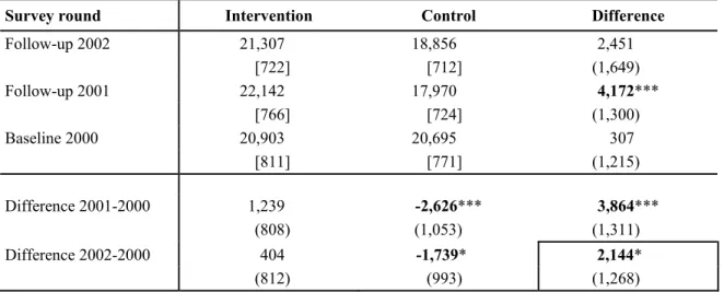
Table 5 shows the average effect of RPS on nominal annual total household expenditures, as measured by the double-difference methodology.19 The control column shows that in 2000, before the program began, average annual total household
expenditures in the control areas were C$20,695. A year later, expenditures had declined by C$2,626 to C$17,970, but by 2002, they had recovered somewhat, reaching C$18,856. The intervention column shows preprogram annual total household expenditures of
C$20,903 in the beneficiary areas. After one year of operation of RPS, annual total household expenditures had risen by more than C$1,000 to C$22,142, but then fell back to C$21,307 in 2002, only C$404 (less than 2 percent) above the level reported in the 2000 baseline.
Table 5—Red de Protección Social (RPS) average effect on annual total household expenditures
Survey round Intervention Control Difference
Follow-up 2002 21,307 18,856 2,451 [722] [712] (1,649) Follow-up 2001 22,142 17,970 4,172*** [766] [724] (1,300) Baseline 2000 20,903 20,695 307 [811] [771] (1,215) Difference 2001-2000 1,239 -2,626*** 3,864*** (808) (1,053) (1,311) Difference 2002-2000 404 -1,739* 2,144* (812) (993) (1,268)
Source: RPS baseline 2000 and RPS 2001 and 2002 follow-up surveys.
Notes: Standard errors correcting for heteroscedasticity and allowing for clustering at the comarcas level
are shown in parentheses (StataCorp 2001); number of observations are shown in brackets. *** indicates significance at the 1 percent level; ** at the 5 percent level; and * at the 10 percent level.
19 The construction of the expenditure measures is detailed in IFPRI (2001b). We present nominal figures
rather than real inflation-adjusted figures to enable a more direct comparison with the fixed nominal transfer levels.
As shown in the right-hand “Difference” column, before the program began, annual total household expenditures in 2000 were very similar in intervention and control areas (differing by only C$307), indicating that on this measure, the randomization into two groups was effective. One year later, however, that small initial difference had grown to C$4,172, and the net average increase, or double-difference estimate of the effect of the program between 2000 and 2001, was C$3,864 (statistically significant at the 1 percent level). With the partial recovery of expenditures in the control group in the second year, however, the estimated effect of the program declined to C$2,144
(marginally statistically significant at the 10 percent level).20 For comparison, the average value of cash transfers for beneficiary households in the evaluation survey was C$3,500 in the first 12 months of operation and C$3,800 in the second 12 months (as only five of the scheduled six payments were made in each year). Beneficiary households are, on average, spending a large proportion of their transfers on current expenditures (rather than increasing savings, for example), though the fraction spent appears to have been smaller in the second year, perhaps, in part, because it was less necessary as the area underwent a partial recovery compared to 2001. Comparing across the extreme poor, poor, and nonpoor in the sample, we find that the largest estimated double-difference effect was for extremely poor households (over C$3,000 in 2002).
The drop in expenditures in the control group seems to have been due in part to an economic downturn in the areas where RPS was operating and in Nicaragua more
generally. Within the control group, expenditures fell among the poor and nonpoor but
20 This effect is not statistically significant at the 5 percent level, in large part because of the asymmetric
distribution of total expenditures. When we examine the double-difference estimate on the natural logarithm of annual total household expenditures (so that they more closely approximate a normal distribution), it is significant at the 1 percent level. In the text, we present absolute measures to facilitate comparison with the nominal transfer amounts.
held steady for the extremely poor.21 Two events affecting the area included a severe drought in 2001 and a sharp, persistent, drop in international coffee prices, which affected many of the agricultural laborers in that industry (Varangis et al. 2003). The rural
Central Region of Nicaragua was the most affected by these events and was the only region showing an increase in poverty rates between 1998 and 2001 (World Bank 2003). The transfers provided by RPS apparently compensated for income losses during this downturn. While not designed as a traditional safety net program in the sense of reacting or adjusting to crises or shocks, the economic difficulties experienced by these
communities allowed RPS to perform like one, as it enabled households to maintain expenditures during a downturn.
The substantial decline in expenditures in the control areas demonstrates the importance of having a control group in this, or any, evaluation. Control groups help isolate the effects attributable to the program and keep them from being confounded with other, nonprogram factors. Without a control group, the analysis would have mistakenly concluded that the RPS had no effect on annual total household expenditures in 2002 (see C$404 difference over time in the intervention group in the second to bottom row of the first column of Table 5).
The RPS effects on per capita annual total household expenditures are shown in Table 6. Average per capita expenditures in 2000 were just over $300 compared to a national average of nearly $500 in 1999, again emphasizing the relative deprivation of the program areas. Reflecting the pattern in total expenditures just described, combined with no significant changes in household size, the results show a small but insignificant
21 The drop in expenditures in the control group was not due to changes in household size or family
composition (see Table 6 on per capita expenditures). Another possibility is that there were biases in the reporting of expenditures. For example, in control areas, it is possible that nonbeneficiaries who had learned about the program understated expenditures to appear more in need of the program. However, at this stage, the program was being implemented using only geographical targeting, and being more or less poor would not have affected eligibility. At the same time, beneficiaries may be overstating food expenditures knowing that increased expenditures on food was one of the objectives of RPS. The fact that the net change in average expenditures is similar in magnitude to the amount of cash transfers suggests these sorts of reporting biases are not substantially altering the findings. There would be more concern if, for example, changes in expenditures were substantially larger than the transfer.