Two Essays on the Long-Term Consequences of the EITC Program

(1)

Persistent link:

http://hdl.handle.net/2345/3316

This work is posted on

eScholarship@BC

,

Boston College University Libraries.

Boston College Electronic Thesis or Dissertation, 2013

Copyright is held by the author, with all rights reserved, unless otherwise noted.

Two Essays on the Long-Term

Consequences of the EITC Program

(2)

Boston College

The Graduate School of Arts and Sciences Department of Economics

TWO ESSAYS ON THE LONG-TERM CONSEQUENCES OF THE EITC PROGRAM

A dissertation

by ANNA BLANK

submitted in partial fulfillment of the requirements for the degree of

Doctor of Philosophy

(3)

c

copyright by ANNA BLANK 2013

(4)

TWO ESSAYS ON THE LONG-TERM CONSEQUENCES OF THE EITC PROGRAM

ABSTRACT by ANNA BLANK

Dissertation Committee: PETER GOTTSCHALK (Co-Chair) ANDREW BEAUCHAMP (Co-Chair)

ARTHUR LEWBEL

This dissertation examines whether the Earned Income Tax Credit (EITC) program improves long-term labor force participation of its recipients.

The first chapter studies the mechanisms which can generate prolonged effects of wage sub-sidies on employment, wages, job stability and poverty. I model three mechanisms: experience accumulation, heterogeneity in the job offer arrival rates, and the costs of switching in and out of employment. I estimate the dynamic discrete-choice model of employment and program participation using a sample of single women from Panel Study of Income Dynamics. The estimates suggest that the EITC program primarily stimulates part-time employment. EITC recipients do not become self-sufficient over the long-term because part-time experience accumulation does not translate into substantial wage growth. The interaction between EITC and other public assistance programs also makes part-time jobs desirable. Counterfactual experiments reveal that in order to promote human capital accumulation and wage growth, the number of hours worked should become one of the determinants in the EITC payment schedule.

The second chapter estimates the life-long effects of the EITC program on employment decisions of single women. To identify those effects I choose a natural experiment framework and use the discontinuity in the eligibility criteria (and payments) associated with the age of the youngest child in the household. I estimate a model with a conditional (fixed-effect) logistic regression using a sample of single women from Panel Study of Income Dynamics. The estimates suggest that there is no significant life-long effect of the EITC program on female labor force participation. The result is

(5)

robust to the definition of the control group and the length of the estimated long-term effects. This conclusion supports the concerns that low-skilled workers do not accumulate experience required for a better employment opportunities. That being said, EITC should be considered solely as a short-term subsidy rather than a long-term investment into experience accumulation.

(6)

Acknowledgements

Without question, this work would not have been possible without the support of many people, a selection of whom I acknowledge here.

I would like to express my sincere gratitude to my first thesis advisor, Peter Gottschalk, who has patiently worked with me all these years at BC. His enthusiasm, knowledge and guidance helped me in this research. Without his advice and support this thesis would not have been possible.

I am especially grateful to Andrew Beauchamp. His willingness to discuss my work, attention to details and optimistic attitude encouraged me to move forward.

My thanks and gratitude also go to professor Arthur Lewbel. His insight and advice were incredibly valuable not only in my research but also during the job-market process.

I cannot overlook my classmates and students at Boston College. I am especially grateful to Geoffrey Sanzenbacher, Samson Alva, Meghan Skira, Stacey Chan and the entire Labor Lunch group. I would also like to thank Gail Sullivan, the Economics Graduate Programs Assistant for her willingness to help and sense of order.

My deep thanks go to my parents, family and friends. My mom and aunt encouraged my all-around education. My family, which doubled in size during my Ph.D. study, provides me with spiritual support every day. Thanks go to my husband Lev, my son Zyama, and my daughter Dalia. My best friend, Anna Okatenko, is a perfect friend.

(7)

Chapter 1 Long-term Consequences of the EITC

Program

1.1 Introduction

The recent trends in federal budget deficits and increased inequality sparked a new wave of interest in tax reform and poverty reduction programs. The issue of ”dependency versus self-sufficiency” is central to these discussions. In particular, is it possible to move people out of poverty by stimulating employment, promoting wage growth and employment stability among low-skilled workers?

In light of these questions the Earned Income Tax Credit (EITC) becomes relevant. The EITC is a refundable tax credit for low- and medium-income individuals and couples, primarily for those who have qualifying children. This is one of the major programs designed to reduce poverty and provide work incentives in the US. Estimates suggest that EITC lifts about 5 million households out of the poverty each year. In 2009, 27 million of the EITC returns generated a total payment to recipients of about $60 billion.1

Given the size and importance of the EITC program, it is not surprising that the labor economics literature has focused on its effect on labor force participation (Dickertet al., 1995; Grogger, 2003; Hotzet al., 2005; Eissa and Hoynes, 2006). Even though the magnitude of the estimated effect varies,

1_{More than 70% of EITC recipients are single, both in terms of the number of returns and total amount paid; 60% of}

(10)

empirical studies generally find that EITC stimulates employment among single women. For instance, Eissa and Liebman (1996) examine 1986 EITC expansion impact and estimate a 2.4-4.1 percentage point increase in labor force participation (LFP) for single mothers. Meyer and Rosenbaum (2001) estimate an increase in LFP by 7-10 percentage points between 1990 and 1996.

According to the human capital theory, however, increased employment should transfer into wage growth through experience accumulation. Wage growth in turn, could translate into self-sufficiency, a desirable feature of any poverty reduction program. In fact, this argument was used to justify the ”quick labor force attachment” approach - women who take low-paying and part-time jobs will eventually move up to the higher-paying and full-time jobs (Pavetti and Acs, 2001). This motivation was part of the welfare reform in mid 1990’s2and it has still a part of the 2012 election campaign for both parties.3 In fact, Dahlet al.(2009) claim that work encouraged through the EITC program continues to pay off through future increases in earnings.4

Other empirical work has been less certain about the possibility of experience accumulation and its transformation into the wage growth for low-skilled workers. For example, Looney and Manoli (2011) find no effect of additional years of experience on the earnings, wages, or employment opportunities of single mothers in 1990s. This result calls in question whether EITC has positive long-term effects on financial independence.

However, the literature also highlights other channels for prolonged effects of EITC. Blau and Robins (1990) suggest that the job offer arrival rates for employed individuals are higher than for the unemployed. Cogan (1981) proposes the idea of fixed costs of entry into the labor market: the exit from nonemployment to employment is associated with additional adjustment costs. This channel might be especially important for single women with children since their move to employment may require the search for child care arrangements. This paper estimates the long-term consequences of the EITC and evaluates the roles of the above channels. In contrast to the majority of earlier

2

New York Times, June 25, 1988 discusses a new welfare initiative ”... these [welfare reform] expenditures can legitimately be seen as an investment to reclaim people from dependency - something that can’t be said about the present welfare system”. ”Welfare-to-work” is one of the key initiatives in government assistance reforms in the 1990s.

3

Paul Ryan: ”The question before us today – and it demands a serious answer – is how do we get the engines of upward mobility turned back on so that no one is left out.” - speech at Cleveland State University on October 24, 2012.

4

Unfortunately, the estimation strategy chosen in this paper has a number of limitations: (1) it assumes the constant sample composition; (2) it mixes short-term and long-term effects of the program; and finally, (3) it mixes the potential wage growth with the potential growth in the number of hours worked.

(11)

studies, I model part-time and full-time work as well as program participation decisions using a dynamic discrete-choice framework which makes it possible to incorporate important elements into the model: the intertemporal trade-off between current disutility of work and future experience accumulation, and current and future labor market frictions. These features allow for long-term labor market effects of the EITC program that may arise due to wage growth or increased employment opportunities. Program participation decisions make it possible to analyze the program interaction between other forms of public assistance and the EITC. By incorporating these elements into an intertemporal model, this paper estimates the importance of different channels through which EITC affects women’s labor market outcomes over the short and long-term.

The structural parameters of the model are estimated by efficient method of moments using data for 1994-2001 from the Panel Study of Income Dynamics. The sample consists of women, heads of the households, age 21-40 excluding students and disabled.

The estimates are in line with the previous literature and suggest that the EITC program stim-ulates employment among single women. However, it encourages part-time rather than full-time employment. Moreover, some women switch from full-time to part-time work because the sum of EITC and other public assistance payments available with part-time employment offsets the full-time earnings.

Supporters of the ”Work first” (Brown, 1997) strategy adopted by a number of states to move people to employment would argue that any employment generates experience, and ultimately, wage growth. Instead, this paper finds very low returns to part-time experience. This is consistent with the findings of Corcoranet al.(1983) who argue that part-time work experience does not lead to significant wage growth and Hirsch (2004) who explains wage differentials between part-time and full-time employed women through limited work experience and human capital accumulation by part-time workers.

To estimate the duration of the long-term impact of receiving the EITC, I simulate two scenarios from the model: first, EITC is not available at all, and second, the EITC program exists for five years and is then unexpectedly removed. Simulations show that the impact past receipt of EITC vanishes in 2-3 years following program participation. This result is driven by the higher arrival rates of job

(12)

offers for employed workers.

The estimated structural parameters are also used to analyze three counterfactual policy experi-ments: (1) elimination of other forms of public assistance for part-time and full-time workers; (2) an increase in the EITC payments; and (3) separate EITC payment schedules for part-time and full-time workers.

The first experiment is motivated by the observed program interaction and focuses on reducing the appeal of a part-time job in favor of a full-time job. The results emphasize the importance of EITC in the absence of the other programs and predict higher full-time employment in the long-run than in the baseline case. The second experiment is designed to make employment more attractive: the EITC payments are doubled. In this case those who do not work in the baseline move to part-time employment, due to large public assistance available for part-time workers. The first two experiments show that full-time jobs cannot become attractive without changes in the proportion of overall public assistance coming from the EITC. Thus, in the third experiment separate payment schedules are introduced for part-time and full-time workers. It is estimated that threefold increase in EITC benefits for full-time employment will generate 5 percentage point increase in full-time employment in the long-run keeping current other public assistance unchanged.

Some may find these conclusions controversial since under the rules of the third experiment, workers with higher earnings (full-time employees) are eligible for the higher EITC benefits than those who earn less while working part-time. While this may seem to contradict the poverty reduction property of the EITC program, it can achieve the goal of prolonged employment stimulation. While welfare and food stamps are designed purely as poverty reduction measures, the earned income tax credit was originally introduced to promote employment. If part-time employment is found to be only a temporary solution for single women, and full-time employment creates better ground for self-sufficiency, then the EITC should also aim to encourage full-time work.

The rest of the paper is organized as follows. The model is presented in Section 1.2. Section 1.3 describes the data and provides descriptive statistics. Section 1.4 discusses estimation method. Results and counterfactual experiments are presented in Sections 1.5 and 1.6. Section 1.7 offers some final thoughts.

(13)

1.2 Model

In this section I present a dynamic discrete-choice model of decision making for a single woman with and without children. In each period a woman makes two decisions: whether to work full-time, part-time or to stay nonemployed,e={0,1,2}, and whether to participate in the public assistance programs or notb = {0,1}. Individuals maximize their life-time utility given time and budget constraints and taking into account the probabilities of job offers and pregnancies.5 The model is solved by backward recursion with expected values calculated using Monte Carlo simulations.

1.2.1 Preferences

Agents in the model are forward-looking. In each period,t, an individual of ageachooses the optimal pairdat ={eat, bat}to maximize her expected life-time utility,Uat

max dat∈Dat ( Uat =E " _A X ea=a δea−au d e at #)

whereDatis the decision set for a person of ageaat timetwhich depends on the set of available

job offers and the number of children;6 δ is the discount factor;udat is the woman’s one-period

utility function given that choicedatis made. The utility functionudat is determined by individual’s

consumption,cat, leisure time,Lat, participation in the public assistance programs,bat, and the costs

of switching between employment options,e_at,₍a−1)(t−1). Public assistance enters the utility function directly to allow for social stigma (Keane and Moffitt, 1998) associated with participation in such programs.7

The utility function is assumed to be log-linear in consumption and leisure; the other arguments enter the utility as additive components:

uat =u(lncat,lnLat, bat, eat,(a−1)(t−1), ε

e,b at)

5

Fertility decisions are considered to be exogenous to the EITC program.

6_{In the model public assistance is not allowed for women without children.} 7

This model is built specifically for public assistance which goes through welfare and food stamps programs. Disutility from using such programs may also come from time-consuming and annoying application process. EITC program is not associated with participation costs since this tax credit becomes available once the standard tax form is completed.

(14)

whereεe,b_at is a time-varying individual-specific unobserved utility from each choice in the model. Unobserved utility is assumed to be i.i.d. with a covariance matrixΣu to be estimated. The full

specification for utility function is presented in the Appendix.

1.2.2 Time and Budget Constraints

Leisure time is defined as a time remaining after completing all job arrangements:

Lat=T−heat,

whereT is the total time available throughout the year;heat _{is hours spent for part-time or full-time}

job att.

Consumption is defined as a sum of after-tax income and public assistance.8

cit=yit−xit+fit=heitwit−xit+fit.

Here,yitis earned income calculated as a product of wage ratewitand hours workedheit;xitis a

sum of income tax and payroll tax,9andfitis the amount of public assistance if available.

1.2.3 Wages and Public Assistance

Individual’s offered wage rate is a function of individual’s full-time experience,X2,tand

part-time experience,X1,t;10time-invariant education leveled; previous period employmentet−1 and current employment optionet. εwte is an i.i.d. normally distributed employment-specific wage

unobservable with mean zero and covariance matrixΣ2_w. Intuitively, it is expected that the wage grows with experience and the education level and is lower for part-time jobs and for those who were recently unemployed. Two separate equations are used for part-time and full-time wages (e∈ {1,2}).

8

Since low-income single women are usually financially constrained, savings and borrowings are not allowed in the model. This assumption simplifies the budget constraint by eliminating inter-temporal substitution.

9

Payroll tax (FICA) includes Social Security and Medicare payments.

10

(15)

lnwe_t =γ₀e+γ₂₁e X2,t+γ22e X22,t+γ11e X1,t+γ12e X12,t+ 2 X j=1 γ_ede jI(ed=j)+γ e e−1I(et−1 = 0)+ε we it .

Low-income households11_{with children are eligible for government support. The amount of} public assistance depends on the number of childrenkt and employment statuset; ft is an i.i.d.

normally distributed public assistance unobservable with mean zero and varianceσ_f2. Softis given

by:      lnft=γ₀f +γf_k₂I(kt= 2) +ft ifet= 0, lnft=γef1+γ f k2eI(kt= 2) +γ f e2I(et= 2) +tf e ifet∈ {1,2}.

I assume thatfitis a sum of the welfare payments12and the food stamp value. This simplification

reflects the fact that in the framework of this model these two programs are indistinguishable: program participation generates extra income, and thus consumption, but also creates negative utility from social disapproval and the application process.13

1.2.4 Job Dynamics and Fertility

Job search frictions are introduced in the model through the job offer probability being less than one and varying across women. The previous period employment option is available in the current period with certainty while the availability of another option is uncertain. The offer arrival rates follow a logistic distribution and depend on the previous period employment status (E₍a−1)(t−1)= 0) as well as current full-time and part-time experiences (X1,atandX2,at).

λe_at= exp

{λe₀+λe_nwI(e₍a−1)(t−1) = 0) +P2j=1λeXjXj,at} 1 + exp{λe₀+λe

nwI(e(a−1)(t−1) = 0) +P2j=1λEXjXj,at}

e∈ {1,2}.

The presence of children in the household affects the employment decisions as well as program participation. The model allows for single women with zero, one and two and more children make

11

Low-income households here are defined as households with before-tax earned income lower than doubled poverty threshold.

12_{Welfare payments are payments associated with AFDC program before 1996 and TANF program after.} 13

The model does not allow for other types of non-labor income: investment income, child support (availability rate is less than 4%), child tax credit (the same for everybody and does not alter employment and program participation decisions), supplemental security income (women in the sample are not eligible) and unemployment insurance (availability rate is less than 5%).

(16)

different decisions.14katis the number of children in the household wherekat ∈ {0,1,2}. Fertility

decisions are considered to be exogenous to the EITC program which is supported by the findings of Baughman and Dickert-Conlin (2003) and Baughman and Dickert-Conlin (2009).

The pregnancy rate is also assumed to follow a logistic distribution and to depend on woman’s ageat, educationedand the current number of children in the householdkat.

φk_at = exp{φ k 0+ P2 j=1φkjI(ed=j) +φk3at} 1 + exp{φk₀ +P2_j₌₁φk_jI(ed=j) +φk₃at} k∈ {0,1}.

A woman knows her future pregnancy probabilities for every age. The pregnancy rates are estimated outside of the model and logit estimation results are presented in Table 1.6.

1.2.5 Dynamic Optimization Problem

In order to solve dynamic optimization problem it is convenient to represent the lifetime utility maximization problem in terms of value functions. A valueVat(Sat)today is a function of current

stateSat15and is determined by the current period decisiondat.

Vat(Sat) = max dat∈Dat

[Vdat(Sat)]

whereVdat(Sat)is a choice-specific expected lifetime value function which can be defined through a

Bellman equation: Vdat(Sat) =      udat +βE(V(a+1)(t+1)(S(a+1)(t+1)|dat ∈Dat, Sat)) ifa < A, udat ifa=A.

TheVdat(Sat)value of any decisiondatis a function of the period utilityudat and the discounted

expected value of future decisions given the current period choice dat. Expectations represent

uncertainty about future income shocks, realizations of utility unobservables, job offer probabilities

14

This assumption is based on the EITC rules which allow different payments for these three categories of households.

15

Two subscriptsaandtrepresent individual’s age and calendar year, respectively. This cumbersome notation is necessary because identical individuals of ageaobserved in yearst1andt2faces different taxes and public assistance policies as well as different EITC schedule and CPI. These changes in economic environment may affect individual’s decisions.

(17)

and potential pregnancies. I assume that individuals have naive expectations about future CPI, taxes and policy changes: in yeartfuture values are calculated keeping the CPI, taxes and policies in all further years at the level of the current year.

The vector of state variablesSatfor a woman is characterized by observable and unobservable

characteristics. Observable state variables are woman’s education leveled, the number of children she haskat, her previous period employmente(a−1)(t−1), her accumulated full-timeX2atand part-time

X1atexperience, her ageatand current tax yeart. Unobserved state variables include realized wage

and welfare shocks as well as unobserved utility arguments.

Sat ={ed, kat, e(a−1)(t−1), X1at, X2at, at, t;εat}.

1.2.6 Solution Method

The dynamic programming problem is solved numerically by backward recursion. In the last period, expected values of the optimal choice are calculated for each reachable state spaceSAT and

each potential choice set using Monte Carlo simulation. For each perioda < Aexpected values are calculated given optimal choices for perioda+ 1. Current period optimal choices are made based on future expected values and current information.16

1.2.7 Identification

Variation in individual outcomes and choices, exclusionary restrictions and parametric assump-tions help identify the structural parameters of the model. A typical identification problem in job search models is to separately identify the parameters of the job offer rates, the parameters of the utility function, and the parameters of the wage equation. Since rejected job offers are usually unob-served, it is hard to distinguish the case of job rejection from the case of no offer. Moreover, since only accepted wages are observed, the distinction between a low wage offer and a high preference for leisure becomes problematic as well.

Several strategies are used to solve this problem. The first one is exclusionary restrictions. For

16

(18)

example, offered wage depends on linear and squared full-time and part-time experience while utility of leisure does not and job offer rates depend on experience only linearly. The second assumption is that the job destruction rate is zero which allows the identification of the job offer arrival rates: part-time (full-time) employees have an option to stay in part-time (full-time) employment for the next period. This assumption means that the utility of leisure can be identified from observing workers who move from employment to nonemployment: it is known that these workers have a job offer but choose nonemployment. Given the estimated utility of leisure, one can identify job offer probabilities by observing transitions from nonemployment to full-time and part-time work, and transitions between employment types.

The utility of the public assistance programs and the parameters of the public assistance amount are identified through the variation in the size of the accepted public assistance. While utility parameters are pinned down by the proportion of individuals who use these programs, parameters of the public assistance amount are determined by the size of the accepted government help.

1.3 Data

The Panel Study of Income Dynamics (PSID) is a primary source of data in this paper. This study started in 1968 with a nationally representative sample of over 18,000 individuals living in 5,000 families in the United States. Information on these individuals and their descendants has been collected continuously, including data covering employment, income, marriage, childbearing and education.

To answer the questions posed above we need data which satisfies several requirements. Firstly, it should be a survey long enough to estimate long-term effects. SIPP, a natural choice for estimating effects of different programs, is not an ideal survey here because a wave length is not long enough. Second, it should contain information about employment choices, wages and a job history. Third, program participation data should be available. Finally, EITC and other tax information is necessary to estimate the model. PSID allows for retrieving demographics, the job history and program participation data. EITC and tax information is calculated through TAXSIM application provided by NBER (Feenberg and Coutts, 1993).

(19)

A potential problem with PSID data is the biannual nature of the data collection in recent years (starting from 1997). Together with the definition of the experience variable in PSID this often leads to considerable limitations in using PSID in dynamic discrete-choice model estimation.Unfortunately, this issue limits the time range suitable for this study to 8-year window: the model is estimated using years 1994 to 2001.17

The sample is restricted to single women with or without children who are between the ages of 21 and 40.18 The model is estimated on core sample data only. Observations with missing welfare information are excluded.19 In addition, any individual who reports disability or school participation is excluded. The final panel consists of 1308 individuals with 4335 person-year observations.

1.3.1 Experience, Employment and Earned Income

PSID is not designed to provide detailed information about job transitions and employment history. This creates a potential problem with using the survey for dynamic discrete-choice estimation with experience being a state variable. For example, the experience variable in PSID is recorded for the head of the household only in years when person becomes a head of the household. Thus, experience needs to be recovered for years when an individual continues to be the head of the household. I calculate individual’s experience using reported annual hours worked and reported earned income.20 Employment is expected to generate income, so only those who report earned income are considered to be employed. The threshold between part-time and full-time employment is set at 1500 hours worked per year (based on a definition of full-time job as at least 30 hours for at least 50 weeks per year). Experience dynamics are recovered from the initially reported full-time and part-time experience and observed employment dynamics. In the model, full-time employees are assumed to

17_{Supplementary files on employment choices and program participation are used to recover hours of work and program}

participation for 1998 and 2000.

18_{The choice of age 40 as an upper limit is somewhat restrictive, but it is required for computational tractability. For the}

older women the state space should also include the set of children ages since some of the children leaves the household altering EITC eligibility. Unfortunately, such expansion of the state space is not feasible at this point.

19

These restriction excludes a lot of high-income individuals from the sample and lowers the average earnings which allow focusing on the low-income women. This is a desirable restriction because one could expect that high-income workers have different decision process from low-income workers, and thus, may distort estimation results.

20

This can be done through an individual’s observed employment status. However, employment question asks about an individual’s current employment status rather than accumulates information about annual work experience.

(20)

work 2000 hours annually, while part-time employees work 870 hours per period.21 Since the model is written for annual data, the total time available for individual is calculated to be 5840 hours per year (16 hours of active time a day multiplied by 365 days a year).

Earned income is defined as ”Head’s of the household labor income”. I drop top 5% of the observations to eliminate outliers and to focus more on the low-income households. Hourly wages are recovered from reported earned income and annual hours worked.

1.3.2 Other Income Variable: taxes, public assistance, and EITC eligibility

PSID is not connected to IRS tax forms, and thus, does not provide tax information including EITC participation. Instead, I use EITC eligibility. EITC eligibility requirements are straightforward and can be used to calculate individual EITC payments. National EITC participation rate estimates range from 75% to 85% of eligible workers (Plueger, 2009). Moreover, some evidence suggests that participation rates for groups with larger tax credits is higher: (1) ”IRS research found that in tax year 1996, the average credit claimed by eligible taxpayers was $1,384, while the average credit available to eligible nonfilers was $1,015” (Berube); (2) participation rates for households with one or two children is close to 100% (White, 2001). This partly justifies the use of EITC eligibility instead of the actual EITC participation. Furthermore, it is interesting to estimate the overall effect of the program given the nonparticipation.

TAXSIM program is used to estimate individual’s income tax, EITC and payroll tax. Since this application is written to process earned income in nominal terms, all monetary variables remain nominal. However, in the model individual’s utility function combines consumption with leisure and other non-monetary components, and thus, requires consumption to have real representation and to be deflated with the consumer price index (CPI).

I use two major sources of public assistance for single women with children are welfare (ADC before 1996 and TANF after 1996) and food stamps (SNAP). PSID has detailed monthly reports of program participation for both. Annual public assistance is calculated as the sum of the food stamps and the annual welfare payments. It is set to zero for women without children since both programs

21

(21)

are designed to support families with children.

1.3.3 Descriptive Statistics

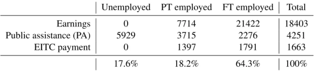
Table 1.1 provides means for earned income, the amount of public assistance and EITC payments by employment status. Notice that the sum of public assistance and the EITC payments falls as employment increases. EITC does not substantially reward full-time employment.

Almost half of part-time workers participate in public assistance and almost 90% of them are EITC eligible (see Table 1.2). Overall, about 30% of single women in the sample use public assistance and about 50% of them are eligible for the EITC.

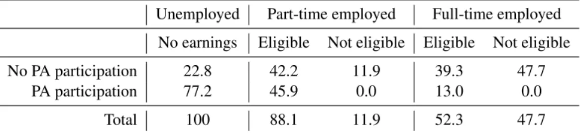
Table 1.3 reports the joint distribution of public assistance participation and EITC eligibility. One third of women who are eligible for EITC participate in public assistance programs. Moreover, if the same statistic is calculated by employment type, the data indicates that among those who work part-time as many as 45.9% are eligible for the EITC and participate in the public assistance simultaneously. This fact highlights the importance of program interaction for an individual’s employment decisions.

Finally, table 1.5 provides basic information about EITC eligibility for women with different education levels and with different family composition. As expected, the EITC program is mostly important for low-skilled women (over 55% of women with high school degree or below are eligible for EITC) or women with children (over 65% of women with one child and over 71% of women with two or more children are eligible for the program).

1.4 Estimation

The estimation of the model presented in Section 1.2 encounters two problems. First, dynamic discrete-choice models usually cannot be solved analytically and require simulations. Second, the missing state variables cannot be ignored. In a likelihood-based estimation approach, the solution is the integration over the distribution of the missing state variables. Since the missing observations include elements of the state space that take on many values (e.g., two types of experience), this approach poses a huge computational burden.

(22)

Therefore, the model is estimated using the efficient method of moments (EMM) which is a generalization for the method of simulated moments (Gourierouxet al., 1993; Gallant and Tauchen, 1996). The moment equations of the EMM estimator are based on the score vector of auxiliary models. Auxiliary models are estimated on the actual data and are chosen to provide a good statistical description of the data. The choice of auxiliary models is driven by the structural parameters of the model and by the set of variables in a state space. Following van der Klaauw and Wolpin (2008), two types of auxiliary models are used in the estimation: first, approximate decision rules that link endogenous outcomes of the model and elements of the state space (e.g., the employment decision), and second, modified structural relationships (e.g., the wage equation). A brief description of the EMM is presented in the Appendix.

1.4.1 The Auxiliary Statistical Models

The choice of the auxiliary model is crucial for identification of the model. The following 74 auxiliary models was used in estimations.22

1. Regressions of log accepted wages on combinations of linear and squared full-time and part-time experience, and education indicators estimated for all employed workers, by employment status and by the number of children.

2. Regressions of log public assistance on combination of age, age squared, indicators for the number of children and employment type indicators.

3. Logits of employment on combination of linear and squared full-time and part-time experi-ence, education indicators, indicators for last period’s employment decision estimated for all employed workers and by the number of children.

4. Logits of program participation on a combination of indicators for employment, education and the number of children as well as previous program participation and previous employment status.

22

Because the auxiliary models do not represent behaviorally interpretable parameters, their estimates are not presented in the paper, and are available on request

(23)

5. Logits of EITC on combination of indicators for employment, education and the number of children as well as previous period EITC eligibility.

6. Multinomial logits of employment on a combination of linear and squared full-time and part-time experience, education indicators, previous period employment status and previous period program participation.

7. Logits of work transitions (job to unemployment and unemployment to job) on a combination of linear and squared full-time and part-time experience, indicators for education and the number of children.

8. Multinomial logits of transitions from unemployment to no work, part-time or full-time work, from part-time work to no work, part-time or full-time work, and from full-time work to no work, part-time or full-time work on combination of linear and squared full-time and part-time experience, education indicators, and last period program participation.

Based on these auxiliary models, 326 score functions are calculated. Those scores are used to identify 47 parameters including parameters of the utility function, job offer probabilities, wage offers and public assistance levels.

1.5 Results

1.5.1 Parameter estimates

Tables 1.7 and 1.8 provide a subset of the parameter estimates. The estimates imply that consumption and leisure are substitutes,αL>0, and that the marginal disutility of hours of work is

greater for those who have children,αEi1 < αEi0andαEi2 < αEi0 fori= 1,2. Transiting from nonemployment to work is costly:αtr <0.

The estimates of the job offer probabilities underscore the importance of the labor market frictions. The probability of receiving a part-time offers starts from 23% per year for those who do not have market experience and goes up to 76% for those who have median experience: two years of part-time experience and six years of full-time experience. The probability of receiving a full-time offers starts

(24)

as low as 4% for those who do not have market experience and goes up to 82% for those who have median experience. The negative effect of nonemployment on the probability of receiving a job offer is larger for full-time offers than for part-time offers, but the magnitude of both effects decrease with experience accumulation.

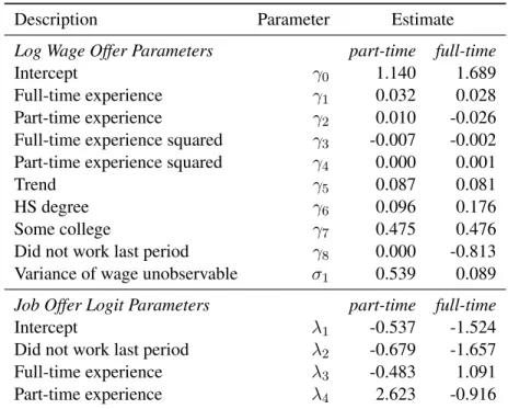
With respect to the estimates of the wage offer function, education has a larger effect on wages for those who work full-time. Person with some college education may expect higher wages than high school graduates. Returns to part-time and full-time experience are very different. The maximum return to full-time experience is achieved at four years of full-time experience for part-time work and at 14 years of full-time experience for full-time work. Return to part-time experience is negative for full-time jobs and about 1% wage increase per year of experience for part-time job.

The parameters of public assistance equation suggest that the second child increases the payments by 42% for nonemployed workers and by 57% for employed. Full-time employment reduces the payments by 88% compared to payments for those employed part-time.

1.5.2 Model fit

The estimated parameters of the model are used to simulate data consistent with the model specification. The simulated data should fit the actual data well in the major descriptive statistics: the proportion of individuals working full-time, part-time and nonemployed; the proportion of individuals who use public assistance; the proportion of individuals eligible for EITC program. Table 1.9 provides evidence on the within-sample fit of the model in these tabulations. The model predictions match the observed fact that women with children are less likely to work and more likely to be in part-time work than women without children; multiple children make those relations even more noticeable. Moreover, women with multiple children have a higher probability for participating in the public assistance programs, while the probability of being eligible for EITC program stays roughly the same.

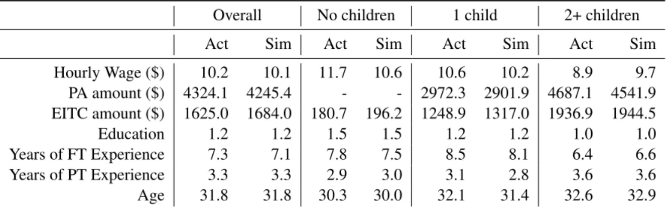
It is obviously important that the model captures the structure of payments. Table 1.10 reports actual and simulated means for the wage, the amount of public assistance, the EITC payments, and for the state variables. The mean hourly wage decreases with the increase in the number of children

(25)

in the household. This may reflect the effect of the lower employment among mothers as well as the effect of selection into the number of children by education (education, on the one hand, has a positive effect on wages, and on the other hand, reduces the probability of pregnancy at each fixed age). Reported education levels confirm this type of selection since the mean education among those who do not have children is higher than among those who have.

Average years of full-time experience are higher for women with one child. This result is not surprising because women with one child on average are 1.8 years older than there counterparts without children; the difference in full-time experience is only about 0.7 years in actual data. Interestingly, average years of part-time experience are higher for women with two and more children. This may reflect the larger disutility of full-time jobs for women with multiple children.

The data on the public assistance amount and on the EITC amount is matched well both, overall and by the number of children. Clearly, women with children depend more on government programs than those without children.

Table 1.11 reports statistics on the actual and predicted distributions of wages. This aspect of the data is crucial for the analysis of the EITC program because the whole distribution of wages, not the mean wage, determines the amount of EITC payments. The large degree of inequality in the wages is clear from the table. Full-time wages are considerably higher than part-time wages.

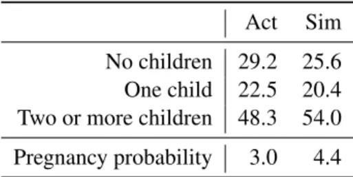
Table 1.12 reports the distribution of children and the pregnancy probability. In the current version of the model, pregnancy rate parameters are estimated outside of the model and come from the simple logit for pregnancy.

1.6 Counterfactual Experiments

Once the model parameters are estimated and the model fit is confirmed, the structural parameters can be used for program evaluation and for counterfactual experiments. The logic of this section is the following. For each evaluated policy three scenarios are simulated: (1) the EITC program is available for the whole period of observations - eight years - Actual EITC; (2) the EITC program is not available for the whole period of observations; and (3) the EITC program is available for the first five years of observations and is shut off for the last three. Individuals, who were eligible for

(26)

the EITC program for at least three years,23form the subsample of interest. Individual decisions under the described three scenarios are compared. Long-term effects of the program are estimated as a difference in observed dynamics for the last three years between scenarios ”No EITC” and ”5 year EITC availability”. That is, long-term effects are observed if the latter does not converge to the former.

The four subsections below discuss the effect of the EITC program on employment, evaluation of the wage changes is not presented here.24

1.6.1 Baseline predictions

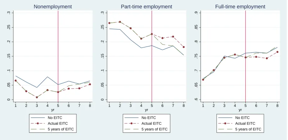
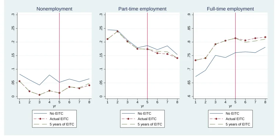
Figure 1.1 reports nonemployment, part-time and full-time employment for the three described scenarios. In the short-run the EITC program reduces nonemployment through the growth of part-time employment; the proportion of full-part-time jobs remains unchanged. In the long-run when the EITC program is shut off (the part of the graph to the right of the red vertical line), employment proportions return to the no EITC level . Low return to part-time experience explains this dynamics: lack of wage growth does not make it possible to maintain the new nonemployment level. However, the higher probability of part-time job offers extends the effect of EITC for one period.

The baseline employment prediction together with the estimated parameters of the wage equation (Table 1.8) suggest that long-term effect of the program might be generated through full-time experience accumulation. The three counterfactual experiments are designed to study the ways to stimulate full-time employment. First, I restrict the use of public assistance to nonemployed individuals with children. Second, I unilaterally increase the amount of the EITC payments. Third, I change the amount of the EITC payments such that, given the same earned income level, full-time workers receive higher payments than part-time workers.

23

More precisely, the subsample consists of individuals who were eligible for the EITC program for at least three years out of the first five.

24_{If the average wages are compared for all employed workers across three scenarios, then the observed wage dynamics}

mixes the effect of sample composition and the effect of wage change. Since the difference in the sample composition between ”No EITC” and ”5 year EITC availability” is in those who do not work under ”No EITC” (mainly because of the low wage offers), the average wage under ”5 year EITC availability” is lower than under ”No EITC”. If the issue of sample composition is addressed through the exclusion of those who have different employment status under these two scenarios, the average wages become practically identical. Finally, the wage comparison for those who work only under ”5 year EITC availability” is meaningless because their wage is unobserved in ”No EITC” scenario.

(27)

1.6.2 Public assistance restrictions

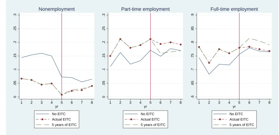
The explanation for the observed EITC effect in baseline case partly comes from the interaction between EITC and public assistance benefits. This is especially true for part-time workers (remember that 45% of them are eligible for EITC and use public assistance - table 1.3). Given the average amount of public assistance for part-time workers, removal of public assistance for part-time workers becomes the first solution to be checked.

More specifically, in this experiment public assistance is shut off for all employed individuals. The results are presented in Figure 1.2. The direct result of this program is increased role of the EITC: in no EITC scenario nonemployment rate is substantially higher than in the previous simulations.25 The interesting effect is observed when 5 years of EITC availability is compared to actual EITC. After the EITC program is shut off, part-time employment decreases, full-time employment increases, keeping the proportion of those who do not work practically unchanged. Intuitively, part-time employment provides much lower earned income than full-time employment (Table 1.1), and under the rules of this experiment when EITC becomes unavailable, and other sources of income are absent, full-time jobs become more attractive.

1.6.3 Unilateral increase in the EITC payments

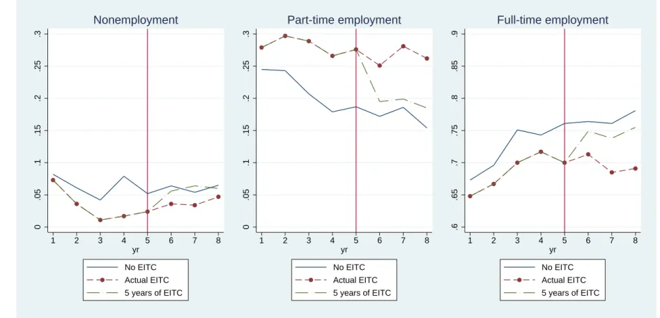
The alternative solution for the observed adverse effect of the program interaction is to increase EITC payments. This should have a positive effect on employment and potentially might make full-time employment more attractive. In this experiment EITC payments are doubled unilaterally for all workers eligible for EITC.26The eligibility criteria remain unchanged.

Employment dynamic for this experiment is presented in Figure 1.3. In the short-run increased EITC payments in fact stimulate employment (nonemployment rates fall). However, this negatively affects full-time employment and happens purely through increase in part-time employment. It is not

25

The counterintuitive dynamics of nonemployment under ”EITC0” is explained by the simulation strategy. In simulations yr 4 corresponds to the taxation year 1996 - the last year before the welfare reform. The simulations predict much higher nonemployment rate before the reform when welfare money could be received pretty easily. The next revision of the paper will include the improved version of the simulation strategy.

26

In the presented counterfactual experiments I abstract from the policy budget issues and consider these exercises as a learning tool which shows the direction of changes, provides some intuition for these directions and estimates the duration of the EITC consequences.

(28)

surprising, that observed long-term effect on employment is small: nonemployment immediately returns to no EITC level, part-time and full-time employment do not match it but move really close.

1.6.4 Increase in the EITC payments for full-time workers

This somewhat unexpected result leads to the third experiment: change the incentives within EITC program. More specifically, EITC payments are tripled for full-time workers and remain unchanged for part-time workers. It is worth mentioning that the logic of this experiment contradicts the current logic of the program: EITC payments are calculated based on the earned income amount and do not take into account the number of hours worked.27 _{The expectation is that supplementary} benefits for full-time workers will attract more women to full-time jobs, and thus, lead to extra full-time experience accumulation. This, in turn, will boost wages and lead to long-term employment stability.

Figure 1.4 presents the employment dynamics under this experiment. The short-term effect of EITC is clearly shifted towards full-time employment. It is interesting that the proportion of part-time workers under no EITC and under actual EITC is almost the same. Reduction in nonemployment goes directly to full-time employment.

The long-term effect of the policy goes in line with predictions. Employment dynamics under 5 years of EITC availability is barely different from the dynamics under actual EITC which means that individuals continue the stay within the same employment type even after the EITC program is stopped.

1.7 Conclusion

This paper proposes and estimates a dynamic model of employment and program participation decisions for a subsample of low-income women from the Panel Study of Income Dynamics. The model was used to estimate long-term consequences of the EITC as well as to understand the mechanisms through which EITC stimulates current employment. The effects of the changes in the

27_{The implementation of the proposed EITC schedule may be problematic since the income forms reported to IRS by}

(29)

EITC schedule and in the other programs are evaluated using counterfactual experiments.

The estimated model finds insignificant long-term effect of the program on employment which is noticeable after only about two years. It also highlights the importance of the distinction between part-time and full-time employment. The estimated parameters of the wage equations show that while full-time experience generates human capital accumulation, and thus, wage growth, part-time experience does not increase wages.

Simulations show that the EITC program stimulates part-time, but not full-time employment. The model suggests that this result comes from the interaction between the EITC and other public assistance programs. The relative generosity of these programs under part-time employment dis-courage workers from choosing full-time jobs, and has adverse effect on the long-term profile of the EITC program.

Counterfactual experiments are designed to test different methods to overcome this program interaction property. Unilateral increase in the EITC payments does not improve the long-term employment patterns. In opposite, targeted increase in the EITC payments for full-time work-ers generates additional full-time employment translated into substantial long-term reduction in nonemployment.

(30)

Tables

Table 1.1: Monetary outcomes by employment status, in dollars Unemployed PT employed FT employed Total

Earnings 0 7714 21422 18403

Public assistance (PA) 5929 3715 2276 4251

EITC payment 0 1397 1791 1663

17.6% 18.2% 64.3% 100%

∗

Note: PSID data, sample of single women age 21-40, non-missing welfare information. The total number of observations is 4335. Public assistance is considerable comparing to the EITC payments, especially for part-time workers.

Table 1.2: PA and EITC eligibility by employment status

Unemployed PT employed FT employed Total No PA participation 28.9 54.1 87.0 71.9

PA participation 71.1 45.9 13.0 28.1

No EITC 100.0 11.9 47.7 47.6

EITC 0.0 88.1 52.3 52.4

∗

Note: PSID data, sample of single women age 21-40, non-missing welfare information. The total number of observations is 4335. EITC eligibility is very high for part-time workers.

Table 1.3: Joint distribution of PA participation and EITC eligibility No earnings Eligible Not eligible Total No PA participation 2.6 34.6 34.7 71.9 PA participation 10.3 17.8 0.0 28.1

Total 12.9 52.4 34.7 100

∗

Note: PSID data, sample of single women age 21-40, non-missing welfare information. The total number of observations is 4335. Program interaction is important: one third of all workers eligible foro EITC is participating in public assistance.

(31)

Table 1.4: Joint distribution of PA participation and EITC eligibility by employment status Unemployed Part-time employed Full-time employed

No earnings Eligible Not eligible Eligible Not eligible No PA participation 22.8 42.2 11.9 39.3 47.7

PA participation 77.2 45.9 0.0 13.0 0.0

Total 100 88.1 11.9 52.3 47.7

∗

Note: PSID data, sample of single women age 21-40, non-missing welfare information. The total number of observations is 4335. Program interaction is extremely important for part-time workers: almost half of all part-time workers both participate in public assistance and are eligible for EITC.

Table 1.5: EITC eligibility by education levels and the number of children

No earnings Eligible Not eligible Total

Less than HS 32.8 57.8 9.4 100 HS 13.1 59.1 27.8 100 Some College 3.4 40.8 55.8 100 No children 4.9 12.3 82.8 100 1 child 10.1 65.3 24.6 100 2+ children 19.6 71.3 9.1 100 ∗

Note: PSID data, sample of single women age 21-40, non-missing welfare information. The total number of observations is 4335. EITC eligible workers are usually low-educated women with children.

Table 1.6: Probability of pregnancy Coeff St.Err. Age -0.069*** 0.018 High School -0.669*** 0.245 Some College -1.250*** 0.273 1 child 0.790*** 0.215 Constant -0.357 0.563 ∗

Note: PSID data, sample of single women age 21-40, non-missing welfare

information. The total number of observations is 4335. Logit estimation for the probability of getting a new child. *** -significant at 1%.

(32)

Table 1.7: Estimated Parameters

Description Parameter Estimate

Utility Parameters

Leisure αL 2.66

Part-time employment when Kids = 0 αE10 -1.16 Part-time employment when Kids = 1 αE11 -1.85 Part-time employment when Kids = 2 αE12 -1.35 Full-time employment when Kids = 0 αE20 0.10 Full-time employment when Kids = 1 αE21 -1.55 Full-time employment when Kids = 2 αE22 -1.03

Switching costs αtr -1.02

Public assistance participation when Kids = 1 αB11 -0.77 Public assistance participation when Kids = 2 αB12 -0.25 Public assistance participation after the reform αr -1.15

Log Amount of Public Assistance Parameters

Intercept for unemployed γ₀f 8.31

Two kids γ_kf₂ 0.42

Intercept for employed γ_ef₁ 7.46

Two kids γ_kf₂_e 0.58

Full-time employed, dummy γ_ef₂ -0.88

∗

Model parameters are estimated using EMM on a sample of 4335 observations.

Table 1.8: Estimated Parameters

Description Parameter Estimate

Log Wage Offer Parameters part-time full-time

Intercept γ0 1.140 1.689

Full-time experience γ1 0.032 0.028 Part-time experience γ2 0.010 -0.026 Full-time experience squared γ3 -0.007 -0.002 Part-time experience squared γ4 0.000 0.001

Trend γ5 0.087 0.081

HS degree γ6 0.096 0.176

Some college γ7 0.475 0.476

Did not work last period γ8 0.000 -0.813 Variance of wage unobservable σ1 0.539 0.089 Job Offer Logit Parameters part-time full-time

Intercept λ1 -0.537 -1.524

Did not work last period λ2 -0.679 -1.657 Full-time experience λ3 -0.483 1.091 Part-time experience λ4 2.623 -0.916

∗

(33)

Table 1.9: Model fit by the number of children - non-monetary outcomes Overall No children 1 child 2+ children

Act Sim Act Sim Act Sim Act Sim

Unemployed 18.3 20.5 7.93 7.49 14.67 19.06 26.19 28.95 PT Employment 17.7 17.8 14.40 13.74 15.98 15.80 20.51 20.45 FT Employment 64.0 61.7 77.67 78.77 69.35 65.14 53.31 50.60 Public assistance (PA) 30.9 34.9 0.0 0.0 29.1 30.9 50.5 52.9 EITC eligibility 48.3 47.3 11.1 10.2 60.5 61.4 65.1 60.2

∗

Actual and predicted percentage of employment, program participation and EITC eligibility: overall and by the number of children. The comparison is made based on 3,756 non-missing observations.

Table 1.10: Model fit by the number of children - monetary outcomes and state variables Overall No children 1 child 2+ children

Act Sim Act Sim Act Sim Act Sim

Hourly Wage ($) 10.2 10.1 11.7 10.6 10.6 10.2 8.9 9.7 PA amount ($) 4324.1 4245.4 - - 2972.3 2901.9 4687.1 4541.9 EITC amount ($) 1625.0 1684.0 180.7 196.2 1248.9 1317.0 1936.9 1944.5 Education 1.2 1.2 1.5 1.5 1.2 1.2 1.0 1.0 Years of FT Experience 7.3 7.1 7.8 7.5 8.5 8.1 6.4 6.6 Years of PT Experience 3.3 3.3 2.9 3.0 3.1 2.8 3.6 3.6 Age 31.8 31.8 30.3 30.0 32.1 31.4 32.6 32.9 ∗

Actual and predicted means for wage, amount of public assistance, EITC payment amount, and state variables. The comparison is made based on 3,756 non-missing observations.

Table 1.11: Model fit - wage distribution Part-time Full-time Act Sim Act Sim 10th percentile 1.72 2.14 5.00 5.02 25th percentile 3.45 3.78 6.75 6.76 50th percentile 6.67 6.30 10.00 9.60 75th percentile 11.49 10.65 14.00 13.11 90th percentile 20.69 17.38 17.50 17.23 ∗

Actual and predicted distribution of wages by employment status. The comparison is made based on 3,756

(34)

Table 1.12: Model fit - children propor-tions

Act Sim No children 29.2 25.6 One child 22.5 20.4 Two or more children 48.3 54.0 Pregnancy probability 3.0 4.4

∗

Actual and predicted proportions of women with zero, one, and two and more children. The comparison is made based on 3,756 non-missing observations.

(35)

Figure 1.1: Baseline Scenario: Long-term effect of the EITC program on employment 0 .05 .1 .15 .2 .25 .3 1 2 3 4 5 6 7 8 yr No EITC Actual EITC 5 years of EITC Nonemployment 0 .05 .1 .15 .2 .25 .3 1 2 3 4 5 6 7 8 yr No EITC Actual EITC 5 years of EITC Part-time employment .6 .65 .7 .75 .8 .85 .9 1 2 3 4 5 6 7 8 yr No EITC Actual EITC 5 years of EITC Full-time employment 27

(36)

Figure 1.2: Public Assistance Restrictions: Long-term effect of the EITC program on employment 0 .05 .1 .15 .2 .25 .3 1 2 3 4 5 6 7 8 yr No EITC Actual EITC 5 years of EITC Nonemployment 0 .05 .1 .15 .2 .25 .3 1 2 3 4 5 6 7 8 yr No EITC Actual EITC 5 years of EITC Part-time employment .6 .65 .7 .75 .8 .85 .9 1 2 3 4 5 6 7 8 yr No EITC Actual EITC 5 years of EITC Full-time employment 28

(37)

Figure 1.3: Unilateral increase in EITC: Long-term effect of the EITC program on employment 0 .05 .1 .15 .2 .25 .3 1 2 3 4 5 6 7 8 yr No EITC Actual EITC 5 years of EITC Nonemployment 0 .05 .1 .15 .2 .25 .3 1 2 3 4 5 6 7 8 yr No EITC Actual EITC 5 years of EITC Part-time employment .6 .65 .7 .75 .8 .85 .9 1 2 3 4 5 6 7 8 yr No EITC Actual EITC 5 years of EITC Full-time employment 29

(38)

Figure 1.4: Increase in EITC for full-time workers: Long-term effect of the EITC program on employment 0 .05 .1 .15 .2 .25 .3 1 2 3 4 5 6 7 8 yr No EITC Actual EITC 5 years of EITC Nonemployment 0 .05 .1 .15 .2 .25 .3 1 2 3 4 5 6 7 8 yr No EITC Actual EITC 5 years of EITC Part-time employment .6 .65 .7 .75 .8 .85 .9 1 2 3 4 5 6 7 8 yr No EITC Actual EITC 5 years of EITC Full-time employment 30

(39)

Appendix

Utility Function: Full Specification

uat = ln(Cat) +αLln(Lat) +αB,K +αE,K+αrI(t >1996)+

+αtr[I(Eat >0|E(a−1)(t−1) = 0) +I(Eat= 0|E(a−1)(t−1)>0)] +εat,E,B

where αE,K = 2 X e=0 2 X k=0 αEekI(Eat =e)I(Kat=k) αB,K = min{1,k} X b=0 2 X k=0 αBbkI(Bat=b)I(Kat=k), αB0k= 0 EMM Estimator

LetyArepresent actual data andΘAbe a vector of parameters in a set of auxiliary relationships.

At the maximum likelihood estimate,Θb_A, the score of the likelihood function with respect to the actual data must be zero: ∂L(yA,ΘbA)

∂ΘA = 0. LetyB represent the data simulated in the behavioral

model using a vector of parametersΘB. Then the optimal vectorΘb_B should generate such data

yB(Θb_B)that the score functions evaluated at the simulated data are as close to zero as possible:

b ΘB= arg min ΘB ∂L(yB(ΘB),Θb_A) ∂ΘA Λ∂L(yB(ΘB),ΘbA) ∂ΘA .

The weighting matrixΛis a block diagonal matrix, where each of the diagonal matrices is the inverse of the Hessian of an auxiliary model evaluated at the actual data.

(40)

Chapter 2 Life-long Consequences of the EITC

Program

2.1 Introduction

Earned Income Tax Credit (EITC) is an earnings subsidy that was introduced to stimulate employment among low-skilled workers. This is one of the largest and most influential poverty reduction programs in the US1. However, long-term effects of the program are still not fully evaluated. This paper addresses the following question. Are there any life-long improvements in the employment profiles of single mothers as a result of employment stimulating programs?

It is a well-documented fact that the EITC program stimulates short-term employment for single mothers (Eissa and Liebman, 1996; Meyer and Rosenbaum, 2001; Hotzet al., 2005; Eissa and Hoynes, 2006). Over time this extra employment can be translated into better employment opportunities through several channels. First of all, more experience may lead to a human capital accumulation and transfer into a future wage growth. Moreover, the exposure to the labor markets may shorten individual’s unemployment spells by increasing the work experience as well as experience in job search. Finally, employment stimulation may improve working culture, and thus, affect positively both wages and job offer arrival rates (Pavetti and Acs, 2001).

1_{Estimates suggest that the EITC lifts about 5 million households above the federal poverty line each year. In 2009, 27}

(41)

Even though theoretical literature suggests those long-term effects, empirical estimations provide contradicting conclusions. For example, longer experience on part-time jobs may have little effect on future employment patterns because it does not stimulate the human capital accumulation, and thus, does not improve wage profiles. Looney and Manoli (2011) find no effect of additional years of experience on the earnings, wages, or employment opportunities of single mothers in 1990s.

In this paper I study the life-long labor supply response of single women with children to the expansions of the EITC program in 1980s and 1990s. I focus on single women with children because they are the largest group of the taxpayers eligible for the EITC. More than 70% of EITC recipients are single, both in terms of the number of returns and total amount paid; 60% of single women with children receive EITC benefits (Plueger, 2009).

The goal of this paper is to clarify the role of the EITC program in the long-term employment behavior of single mothers. The positive life-long effect of the EITC program may justify the increase in the government-sponsored employment stimulation: the increase in the employment probability of those who are not eligible anymore may reduce the government expenses in other poverty reduction programs such as subsidised housing, food stamps, etc.

The effects of the EITC program on life-long employment are estimated using the framework of a natural experiment. I compare the change in the labor supply of two groups of single women whose children have left the household: the first group includes women who had children during the generous stage of the EITC program and the second group includes women who had children during the moderate stage of the program. At the moment of interest - namely, when the youngest child reaches age eighteen - both groups do not have access to the EITC program because they do not meet the requirement of having children in the household2. However, the exposure to the EITC program in the past for those two treated groups was different.

To define the term ”exposure to the EITC program” the endogeneity issue should be discussed here. Suppose that the sample is restricted to women who actually received the tax credit in the past. Then this sample includes those who would work even without the EITC support but received some monetary supplement and those who would not work without the EITC, but were moved

2

I account for the changes in the labor market conditions between these two periods using the control group of women without children.

(42)

to employment as a result of the program. However, this sample excludes those who were not stimulated by the EITC program and remained non-employed. The selection becomes an issue because individuals may self-select into those groups based on some unobserved characteristics. To address this problem I include in the sample all women who meet all but one (earned income) eligibility requirements and I call these requirements ”exposure to the EITC program”. Thus, the sample consists of women who are potentially eligible to the EITC benefits if they meet the earned income requirement3.

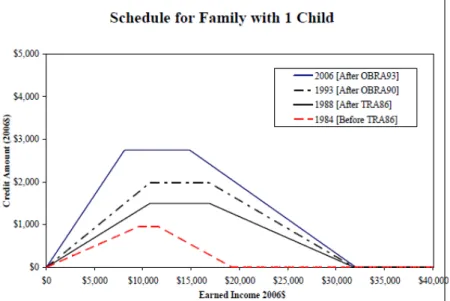
The effects of the EITC program on the long-term employment are estimated on the PSID data using the logistic model with individual fixed-effects. The sample consists of 41209 observations and 5836 of individuals over years 1968 and 2007 and split into four regimes: ”No EITC” - before the introduction of the EITC program in 1975, ”Moderate EITC” - between the introduction and the first major expansion in 1986 (TRA86), ”Transition” - between the two major expansions in 1986 and 1993 (TRA86 and OBRA93), and ”Generous EITC” - after the second major expansion in 1993 (OBRA93)4. The long-term effect is divided into two subperiods: the effect one to five years after the exposure to the program and the effect more than five years after the exposure. The regression controls for demographic characteristics such as age, education level, age of the youngest child, etc.

The short-term effects of the EITC program are estimated to be positive: the EITC program stimulates single women with children to work more. These findings are consistent with the previously documented results (Eissa and Hoynes, 2006; Dickertet al., 1995; Grogger, 2003). The life-long effects of the EITC program are found to be insignificant. The exposure to the EITC in the previous years does not generate higher labor market participation for single woman whose children have left the household.

Several specifications were used to check the robustness of these results. Two different base levels are chosen: the comparison is done against the ”Moderate EITC” regime as well as against the ”No EITC” regime. The division of the long-term effects was modified: the three subgroups include (1) the effect one to five years after the exposure to the program, (2) the effect five to ten years after

3

Historical participation rates for the EITC program are more than 80% and even higher for those who are eligible for maximum credit (White, 2001). That said, it is reasonable to assume that single women who meet all but one requirement are aware of the EITC program.

(43)

the exposure, and (3) the effect more than ten years after the exposure. All those modifications do not alter the results substantially.

Two remarks should be made here. First, unlike the standard natural experiments where the policy change is usually supposed to be unexpected to the program participants, the eligibility change considered in this paper is perfectly predictable and depends on the children’s age. One may argue that predictability of the policy change may affect individual’s behavior and lead to incorrect conclusions. However, the main idea in this paper is to estimate life-long effect of the EITC, and thus, to take into account not only the short-term decisions, but also the decisions which depend on the past and the future anticipated changes in the program. Another possible concern is potential endogeneity. Since the EITC eligibility depends on children’s age, the household may postpone the eligibility lost by changing their fertility choices. That in fact could be a problem, but the empirical literature suggests that both marriage and fertility choices are not affected by the EITC policy (Baughman and Dickert-Conlin, 2003, 2009).

Second, I would like to stress here that I do not estimate the effect of the EITC participation, but rather the effect of the existing EITC rules during the years of active child bearing for single mothers (effect of potential eligibility). There are two reasons for that: (1) it allows me to estimate the actual observed effect in the society, not the hypothetical effect only on those who are directly affected by this program; and (2) it solves the selection problem - actually EITC participants might be different from those who were not receiving EITC payments.

The rest of the paper is organized as follows. Section 2.2 provides brief policy description. Section 2.3 describes the data and presents descriptive statistics. Section 2.4 discusses estimation method and identification strategy. Results and their interpretations are presented in Section 2.5. Section 2.6 offers some final thoughts.