Self-Organizing Map
Jouko Lampinen and Timo Kostiainen Laboratory of Computational Engineering, Helsinki University of Technology,
P.O.Box9400, FIN-02015 ESPOO, FINLAND [email protected], [email protected]
Abstract. The Self-Organizing Map, SOM, is a widely used tool in exploratory data analysis. A theoretical and practical challenge in the SOM has been the diffi culty to treat the method as a statistical model fitting procedure. In this chapter we give a short review of statistical approaches for the SOM. Then we present the probability density model for which the SOM training gives the maximum likeli hood estimate. The density model can be used to choose the neighborhood width of the SOM so as to avoid overfitting and to improve the reliability of the results. The density model also gives tools for systematic analysis of the SOM. A major ap plication of the SOM is the analysis of dependencies between variables. We discuss some difficulties in the visual analysis of the SOM and demonstrate how quanti tative analysis of the dependencies can be carried out by calculating conditional distributions from the density model.
1
Introduction
The self-organizing map, SOM, is a widely used tool in data mining, visual ization of high-dimensional data, and analysis of relations between variables. For a review of SOM applications see other chapters in this volume, and [12]. The most characteristic property of the SOM algorithm [8] is the preser vation of topology, or the fact that the neighborhood relationships of the input data are maintained in the mapping. A large part of theoretical work on SOM has been focused on the definition and quantification of topology preservation, but mathematically rigorous treatment is not yet complete. See [16] for up-to-date discussion of the topology preservation in the SOM.
The roots of the SOM are in simplified models for the self-organization process in biological neural networks [7]. In related engineering problems the SOM offers considerable potential, such as in automatic formation of categories in larger artificial neural systems.
Currently, a very active application domain of the SOM is exploratory data analysis, where a database is searched for any phenomena that are important in the studied application. In normal statistical data analysis there are usually a set of hypotheses that are validated in the analysis, while in exploratory data analysis the hypotheses are generated from the data in a data-driven exploratory phase and validated in a confirmatory phase.
The SOM is mainly used in the exploratory phase, by visually searching for potentially dependent variables. There may be some problems where the exploratory phase alone might be sufficient, such as visualization of data without more quantitative statistical inference upon it. However, in practical data analysis problems the found hypotheses need to be validated with well understood methods, in order to assess the confidence of the conclusions and to reject those that are not statistically significant.
When using the SOM in data analysis, an obvious criterion for model selection should be generalization of the conclusions to new data, just as it is in the case of any other statistical method. The preservation of topology is also important, to facilitate the visual analysis by grouping the similar states to neighboring map units, but if the positions of the map units are not statistically reliable the map is useless for any generalizing inference.
In this chapter we present the SOM as a probability density estimation method, in contrast to the standard view of the SOM as a method for map ping high dimensional data vectors to a lower dimensional space. There are several benefits in associating a probability density, or a generative model, with a mapping method (see [14] for discussion of a generative model for the PCA mapping):
• The density model enables computation of the likelihood of any data sample (training data or test data), facilitating statistical testing and comparison with other density estimation techniques.
• The selection of hyperparameters of the model (eg., the width of the neigh borhood) can be chosen with standard methods, such as cross-validation, to avoid overfitting, in the same way as with other statistical methods.
• The density model facilitates quantitative analysis of the model, for ex ample, by computing conditional densities to test the visually found hy potheses.
• In principle, Bayesian methods could be used for model complexity con trol and model comparison (see [10] for a review of Bayesian approach for neural networks). However, as shown later, the normalization of the probability density in the original SOM requires a numerical procedure that seems to render the Bayesian approach impractical.
The organization of this chapter is the following:
In section 2 we discuss the problem of finding dependencies between vari ables using visual inspection of the SOM, to demonstrate the need for quan titative analysis tools with the SOM.
In section 3 we shortly review some results related to the existence of the error function in the SOM. The SOM algorithm is not defined in terms of an error function, but directly via the training rule, and unfortunately the training rule is not a gradient of any global error function [5]. This makes the exact mathematical analysis of the SOM algorithm fairly difficult. For a discrete data sample the algorithm may converge to a local minimum of an error function [13] , which may exist only in a small volume in the parameter
space (the error function changes if the best-matching unit of any data sample changes). In section 3 we shortly review the results about the existence of the error functions in the SOM and some modifications that make the error function to exist more generally.
The probability density model in the SOM, derived in this chapter, con sists of kernels of non-regular shape, whose positions are weighted averages over the neighboring units receptive fields, and thus the model is close to many mixture models where the kernels are confined to a low dimensional latent space. In section 4 we review some constraint mixture models that are similar to the SOM.
In section 5 we derive the exact probability density model, for which the converged state of the SOM training gives the Maximum Likelihood estimate. In section 6 we discuss the selection of the SOM hyperparameters to avoid overfitting, and demonstrate how quantitative analysis can be carried out with the aid of the probability density model.
In section 7 we present conclusions and point some directions for further study.
2
SOM and Dependence Between Variables
In practical data analysis problems a common task is to search for depen dencies between variables. Statistical dependence means that the conditional distribution of a variable is dependent on the values of other (explanatory) variables, and thus the analysis of dependencies is closely related to the estimation of probability density or conditional probability densities. In re gression analysis the goal is to estimate the dependence of the conditional mean of the target variable on the explanatory variables, using, for example, the standard least squares fitting of neural network outputs to the targets. In real data analysis problems, the shape of the conditional distribution needs to be considered also in the regression models, by means of, e.g., error bars, or confidence intervals, in order to assess the statistical significance of the dependence of conditional mean on the explanatory variables.
The most simple goal is to look for pairwise dependencies, where a vari able is assumed to depend only on one other variable. For such a problem the advantage of the SOM is rather marginal, as simple correlation anal ysis is sufficient for the linear case, and in the non-linear case there exist plenty of methods for directly estimating the conditional density and thus the dependencies in such a low dimensional case (see e.g. [2] for review).
The tough problem in exploratory data analysis is to search for non-linear dependencies between multiple variables. With the SOM, the analysis of de pendencies is based on visual inspection of the SOM structure. Several visu alization methods have been developed for interpreting the SOM, see, e.g., [4]. The basic procedure is to visually search for regions on the map where the values of two or more variables coincide, e.g., have large or small values
in the same units. Such a region is interpreted as a hypothesis that the vari ables are dependent in a way that, for example, low value for one variable is indication of low value for the other variable, given that rest of the vari ables are close to the corresponding values in the reference vectors. Clearly, efficient visualization methods are necessary, as the number of variable pairs is proportional to the square of the number of variables, and there may be dozens of distinguishable regions in the SOM.
It is very important to notice that any conclusions drawn from models overfitted to the data sample are not guaranteed to generalize to any other situation. In the case of the SOM, overfitting means that reference vectors of some units have been determined by too few data points, so that the reference vectors are not representative of the underlying probability den sity. Any conclusions based on such units are prone to fail for new data, and thus analysis of statistical dependencies requires some way, heuristic or more disciplined, to avoid overfitting, as in all statistical modeling. On the other hand, it should be noted that when the SOM is used for analyzing the whole population, and measurement errors are considered negligible, there is no need to generalize the conclusions to other data, and overfitting is not an issue. This important distinction between analyzing the population, and analyzing a sample from the population and generalizing the conclusions to the population, often seem to be ignored in the SOM framework.
The main problem in visual inspection of the SOM is that in general
the lack of dependence between variables is difficult to observe visually from the SOM. That is, even if variables, say, x1 and x2 both have high values at map unit Mij, that alone does not show that the variables have any mutual dependence. As a simple example, consider two-dimensional uniform distribution x1, x2∼U(−1,1). A 2×2 SOM with zero neighborhood would
have component planes (in any order of the columns and rows)
M1= −0.5−0.5 0.5 0.5 M2= −0.5 0.5 −0.5 0.5
The coincidence of high values in unit M22 and low values inM11 are only a result of the vector quantization. To see that high values in M22 do not indicate dependence between x1 and x2, one must observe that high value for x1 occurs also in M12 with low value forx2 (i.e., tallied over the map,
high value forx1occurs with both high and low value forx2).
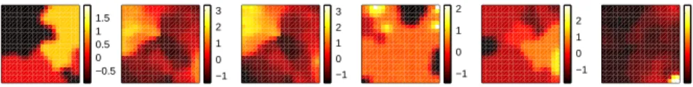
In high dimensional space the visual inspection of the dependencies be comes more difficult, as the map folds into the data space, and the range of values for each variable is distributed around the map. Fig. 1 illustrates this for random data with no dependencies between the variables, and Fig. 2 shows an example from a real data analysis project, where all hypotheses were later rejected in careful analysis.
−2 0 2 −2 0 2 −2 0 2
Fig. 1. Example of a SOM trained on purely random data. The independence of the variables in the component level display is not trivial to observe. One might, for example, erroneously conclude that high values ofx3would indicate low values ofx2. Here the neighborhood is trained down to zero.
−0.5 0 0.5 1 1.5 −1 0 1 2 3 −1 0 1 2 3 −1 0 1 2 −1 0 1 2 0 5 10
Relative humidity Enthalpy Air freshness Ergonomics Carbon dioxide
Allergic history
Fig. 2. Example of real data analysis. In the case study, the dependence of Air freshnesson the other variables was investigated. In the final analysis all hypothe ses were rejected using methods like RBF models, Bayesian neural networks, and hierarchical generalized linear models using Bayesian inference, etc. [17]. One ev ident conclusion, from the lower right corner of the map, is that high value for variable Ergonomics appears only with low value for Air freshness, but careful analysis showed that this was just an effect of vector quantization.
3
Error functions in the SOM
The converged state of the SOM is a local minimum of the error function which is given by [13] E(X) = N n=1 M j=1 Hbjxn−mj2, (1)
where X = {xn}, n = 1, . . . , N is the discrete data sample, j is the index (or position) of a unit in the SOM, with reference vector mj, and Hbj = H(b(x)−j) is the neighborhood function,b(x) being the index of the best matching unit forx.
The error function is not defined at the boundaries of the receptive fields, or Voronoi cells, so the function does not exist in the continuous case. In the case of a discrete data set, the probability of any sample lying at any boundary is zero, so in practice the error function can always be computed for any data set. The error function changes if any sample changes its best matching unit. That is why the error function is only consistent with the SOM training rule when the algorithm has converged. In practical data analysis
the data set is always discrete and the algorithm is allowed to converge, so analysis of the error function is thereby justified.
The SOM training rule involves assigning to each data sample one refer ence vector, the best matching unitb(x). The matching criterion is Euclidian distance, as follows:
b(x) = argmin
i x−mi.
(2) When a sample is near a boundary of two or more receptive fields, a small change in the position of one reference vector can change the best matching unit of that sample. Hence the gradient of the error function with respect to the reference vectors is infinite.
The error function (1) can be thought of as the sum of the distortion function
D(x) = j
Hbjx−mj2. (3)
over the data set. The distortion function is also discontinuous at the Voronoi cell boundaries. The discontinuity is a result of the winner selection rule of the training algorithm.
Luttrell [11] has shown that exact minimization of Eq. 1 leads to an approximation to the original training rule, where, instead of the nearest neighbor winner rule, the best matching unit is taken to be the one that minimizes the value of the distortion function (3), as follows:
b(x) = argmin i
j
Hijx−mj2. (4)
The minimum distortion rule avoids many theoretical problems associated with the original rule, without compromising any desirable properties of the SOM except for an increase in the computational burden [6]. The gradient of the error function becomes continuous at the boundaries of receptive fields (which are no longer the same as the Voronoi tessellation). The distortion function with the modified winner selection rule is also continuous across the unit boundaries.
4
Constrained Mixture Models
The main aspects of the SOM algorithm, that make the analysis difficult are 1) the hard assignment of the input samples to the nearest units, which makes the receptive fields irregularly shaped according to the Voronoi tessel lation, and 2) the regularizing effect defined as updating the parameters of the neighboring units towards each input, instead of regularization applied directly to the positions of the reference vectors.
It is worth noticing that the first issue is due to the shortcut algorithm [7] devised to speed up the computation and to enchance the organization of
the map from a completely random initial state, and is not a characteristic of the assumed model for the self-organization in biological networks. The original on-center off-surround lateral feedback mechanism in [7] produces a possibly multimodal pattern of activity on the map, that was approximated by a single activity bubble around the best-matching unit, BMU, with the shape of the neighborhood function. Then equal Hebbian learning rule in each unit produces the concerted updating towards the input in the neighborhood of the BMU. An interpretation of the mapping of input data point on the SOM lattice, that would be consistent with issues above, and the minimum distortion rule in Eq. 4 would thus be, that a point in the input space is mapped to a activity bubbleHib around the BMUb, rather than to a single unit.
By ignoring the winner-take-all mechanism the SOM can be approximated by a kernel density estimator, where the activity of a unit is dependent only on the match of the data point and the unit reference vector. This is often called soft assignment of data samples to the map units, in contrast to the hard assignment of a data point to only the best-matching unit.
The second characteristic of the SOM training, the way of constraining the unit positions, is dictated by the biological origin of the method. A reg ularizer directly on the reference vector positions would require a means for the neurons to update their weights towards the weights of the neighboring neurons, while in the SOM rule all learning is towards the input data. The biological plausibility is obviously non-relevant in data analysis applications, even though it may have a role in building larger neural system with the SOM as a building block.
In the approach taken by Utsugi [15] , small approximations are made to render the model more easily analyzable: the winner-take-all rule is re placed by soft assignment, and the neighborhood effect is approximated by a smoothing prior directly on the reference vector positions. The model is then a Gaussian mixture model with kernels constrained by the smoothing prior. This approach yields a very efficient way to set the hyperparameters of the model, that is, the widths of the kernels and the weighting coefficient of the smoothing prior, by empirical Bayesian approach. For any values of the hyperparameters, the evidence, or conditional marginal probability of the values given the data and the priors, can be computed by integrating over the posterior probability of the model parameters (kernel positions). The values with the maximum evidence are then chosen as the most likely values. Ac tually, a proper Bayesian approach would be to integrate over the posterior distribution of the hyperparameters (see [10] for a discussion), but clearly the empirical Bayes approach is a notable advance in the SOM theory.
Another model close to the SOM is the Generative Topographic Mapping [1]. In that approach, the Gaussian mixture density model is constrained by a nonlinear mapping from a regularly organized distribution in a latent space to the component centroids in data space. Hyperparameters of the model, which
control noise variance, stiffness of the nonlinear mapping and the prior dis tribution of mapping parameters, can be optimized using Bayesian evidence approximation, similar to the one used by Utsugi [3].
5
Probability density model in the self-organizing map
In this section we derive the probability density model for the original SOM, with no approximations in the effect of the neighborhood or the posterior probability of units given an input sample (the activity of the units).
The density model is based on the mean square type error function (1), discussed in section 3. The error function is specific to the given neighborhood parameters, so that it cannot be directly used to compare maps which have different neighborhoods. The maximum likelihood (ML) estimate is based on maximizing the likelihood of data given the model. We wish to find a likelihood function which is consistent with the error function. This can be achieved by making the error function proportional to the negative logarithm of the likelihood of data. Assuming the training samplesxnindependent, the likelihood of the training set X = {xn}, n = 1, . . . , N is the product of probabilities of each sample,
p(X|m, H) = n
p(xn|m, H), (5)
wheremdenotes the codebook (set of reference vectors) andH is the neigh borhood. The negative log-likelihood is L =−logp(X|m, H) and setting it proportional to Eq. 1 yields
p(X|m, H) =Zexp(−βE) =Zexp(−β n
j
Hbjxn−mj2). (6) Here we have introduced two constants,Z and β, which are not needed in the ML estimate of the codebookmbut which are necessary for the complete density model. The probability density function in Eq. 6 is given by
p(x|m, H) =Zexp(−β j
Hbjx−mj2), (7) which is a product of Gaussian densities centered atmj, whose variances are inversely proportional to the neighborhood function valuesHbj. Note that the discontinuity of the density is due to the discontinuity of the best-matching unit indexbfor the inputx.
Inside a Voronoi cell, or the receptive field of unitmb, the density function has Gaussian form:
p(x|x∈Vb) =Ze−βWbexp − 1 2s2b x−µb2 , (8)
whereVb denotes the Voronoi cell around the unitmb. The position and the variance of the kernel are denoted by µb and s2b, respectively, and Wb is a weighting coefficient. The values of the parameters are
µb= jHbjmj jHbj (9) s2b = 1/(2β j Hbj) (10) Wb= j Hbjmj−µb2. (11)
The density model consists of cut Gaussian kernels, which are centered at the neighborhood-weighted means of the reference vectors and clipped by the Voronoi cell boundaries.
The parameter Wb controls the height of the kernel; it depends on the density of the neighboring reference vectors near the centroidµb. The density function is not continuous at the boundaries of the Voronoi cells. See Figs. 3 , 4 and 5 for examples of the density models. The variances of the kernels depend on the parameter β and they are equal if the neighborhood is normalized (see section 6.1 for further discussion). In the standard SOM formulation, the border units with incomplete neighborhood have larger variances, as can be seen in Figs. 5 and 8 , allowing the map to shrink into the middle of the training data distribution.
The normalizing constant Z and the noise variance parameter β are bound together by the constraint that the integral of the density over the data space must equal one. That integral can be written as
p(x)dx=Z r e−βWb x∈Vr exp(− 1 2s2r x−µr2)dx, (12)
where the integration over the data space is decomposed to the sum of inte grals over each Voronoi cell. The integrals cannot be computed in closed form but they can be approximated numerically using Monte Carlo sampling. A simple way to do this is the following algorithm:
1. For each cellr, drawL samples from the normal distributionN(µr, sr) 2. Computeqr=Lr/L, the fraction of samples that are inside the cellr. 3. The integral over Vrin Eq. 12 equalsqr(2πs2r)d/2, wheredis the dimen
sion of the data space.
For a map that contains M units, this algorithm requires the computation of distances betweenM×Lsamples and theM reference vectors. Thus ifM is large the computational cost of the normalization procedure exceeds that of the training algorithm itself.
In an efficient implementation the number of samplesLshould be chosen according to the desired accuracy. The acceptance ratio qr varies in large
−0.50 0 0.5 1 1.5 2 2.5 0.2 0.4 0.6 0.8 1 1.2 1.4 1.6 −0.50 0 0.5 1 1.5 2 2.5 0.2 0.4 0.6 0.8 1 1.2 1.4 1.6 0.1 0.2 0.3 0.4 0.5 0.6 0.7 0.8 0.9 0.6 0.65 0.7 0.75 0.8 0.85 0.9 0.95 1
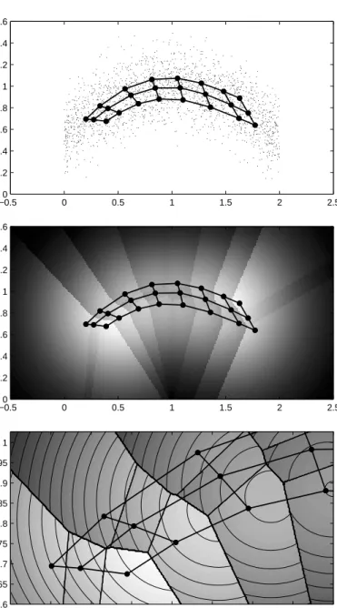
Fig. 3.Example of the density model in a 3×8 SOM. Top: training data and the resulting SOM lattice using Gaussian neighborhood withσ= 1. Middle: the density model of the SOM. Bottom: zoomed part of the density model above, with contours and Voronoi cell boundaries added. From the figure it is clear how the Gaussian kernels are located at the neighborhood weighted averages of the reference vectors.
L = 400 L = 388 L = 414
Fig. 4. Training data and density estimates due to different SOM topologies. L denotes the negative log-likelihood of test data. The optimal value for the parameter β is so small that the model is close to normal Gaussian mixture. Among these alternatives, the 3×6 topology (middle) produces the best model judging by the likelihood criterion.
range according to the neighborhood size. When the neighborhood is small, the neighborhood-weighted centerµris close to the reference vector mrand sr is likely to be small, so qr is high. When the neighborhood is large the situation is opposite, and to achieve an equivalent accuracy L will have to be much greater. Detailed analysis of the dependence of the accuracy on L is presented in appendix A.
The maximum likelihood estimate forβ can only be found by numerical optimization, by maximizing the likelihood of validation data. It is worth noting that when a numerical method such as bisection search is applied, savings can be made by allowing the accuracy to vary. Initial estimates can be very coarse, corresponding to smallL, if the accuracy gradually increases towards the convergence of the search. The final accuracy should reflect the size of the validation data sample.
By equating the partial derivative of the likelihood function ∂p(X)/∂β with zero, an interpretation for the maximum likelihood solutionβmlcan be found in terms of the neighborhood-weighted distortion functionD(x) (3) as
follows: N n=1D(xn) N = D(x) exp(−βmlD(x))dx exp(−βmlD(x))dx . (13) Observe that the estimated input distribution is ˆp(x|β, H)∝exp(−βD(x)). Heuristically, Eq. 13 says that, at the ML-estimate withβ equal toβml, the mean value ofD(x) over the estimated input distribution equals the sample average of D(xn) over the input dataxn, n= 1, . . . , N.
6
Model selection
The SOM algorithm produces a model of the input data. The complexity of this model is determined by the number of units and the width of the
neighborhood, which has a regularizing effect on the model. When the input data is a sample from a larger population, the objective is to choose the complexity such that the model generalizes as well as possible to new samples from that population. See [9] for discussion and examples of overfitting of the SOM model. The likelihood function provides a consistent way to compare the goodness of different models. In this section we discuss how this can be used for model selection in the self-organizing map.
Let us first regard the number of units as given, so neighborhood width σ is the sole control parameter. The density model allows us to select the neighborhood width σ by maximizing the likelihood of data p(X|m, H). In the course of SOM training, σ is gradually decreased in some pre-specified manner, i.e.σ=σ(t), t= 1, . . . , K;σ(t+1)< σ(t). We trust that the training algorithm will find an ML estimate for the map codebook at each value of the neighborhood widthσ(t) , if it is allowed to converge every time. To con struct the density model for each of theseKcandidate maps, we numerically optimize β(t) as described in the previous section. This yields K different density models to compare. To choose between these we compute the likeli hood values p(XV|m(t), σ(t), βml(t)) for validation data XV (which should ideally be different from that used to select βml(t)). Cross-validation can also be applied. An example of model selection is shown in Fig. 5. The map with σ = 1.00 maximizes the likelihood of validation data. This approach extends directly to the comparison of different size maps as well as different topologies (see Fig. 4). If one wishes to have a large map, it may be advisable to ease the computational requirement by finding the correctσfor a smaller map first and then simply scaling it up in proportion to the dimensions of the maps. (For example, ifσKL is the optimal neighborhood width for aK×L map, then 5σKLis probably a reasonable value for a 5K×5Lmap.)
Because the exact value of the density function cannot be computed in closed form, it is difficult to apply methods such as Bayesian evidence to pa rameter selection. If the values of the function itself are approximations, then the derivatives will be even more inaccurate, and due to the numerical nor malization procedure the approach would be computationally too expensive in practice.
A common application of the SOM is to look for dependencies between variables by visual inspection. In that context, the density model can be used to select the complexity of the model, but it also enables quantitative analysis. Regression or conditional expectations can be computed directly from the joint density in Eq. 7 by numerical integration. For example, the conditional distribution for variable xj equals
p(xj|x\j, m, H) = p
(x|m, H) p(x|m, H)dxj,
(14) where x\j denotes the vector x with element j excluded. Likewise, the re gression of xj on other variables can be computed as the conditional mean
σ = 8.30, β = 0.10, L=2.33 σ = 4.90, β = 0.25, L=2.01
σ = 1.00, β = 2.53, L=1.86 σ = 0.20, β = 9.34, L=1.92
Fig. 5. SOM density models for different widthsσof the Gaussian neighborhood. From the total likelihood of validation data the optimal neighborhood can be chosen to avoid overfitting. Ldenotes the negative log-likelihood of validation data (per sample).
E[xj|x\j, m, H]. It should be noted that the SOM density model may not give the best possible description of the input distribution. We have included this discussion here so as to illustrate the value of model selection.
Reducing the variance parameter to zero, β → ∞, gives an important special case. The conditional density is then sharply peaked at the value of the “outputs” xj in the best matching unit for the “inputs” x\j. The condi tional mean E[xj|x\j] then gives the same value as nearest neighbor (NN) regression with the SOM reference vectors, with the neighborhood-weighted reference vectors (Eq. 9) as output values, producing a piecewise constant estimate. Comparison with the NN rule is interesting, because it is a close quantitative counterpart of the popular visual analysis of the SOM.
Fig. 6 illustrates the difference between computing the conditional mean from the density model and using the nearest neighbor rule. A random 3D
data set (∼ N(0,1)) is analyzed by a 6×6 SOM. We attempt to infer E(x2|x1, x3= 0) , the expected value of the variablex2givenx1, withx3zero.
As the variables are truly independent, the answer should beE(x2|x1, x3=
0) =E(x2) = 0. The optimal width of the Gaussian neighborhood function is
σ= 4.2 , which is a relatively large value, suggesting independent variables (a “simple” distribution). At zero neighborhood, the model is badly overfitted. Clearly, neglecting to select the correct model complexity would give unreli able results. When the complexity is right, the nearest neighbor rule can give a good approximation to the mean, though the lack of confidence intervals limits the reliability of analysis.
0.05 0.1 0.15 0.2 0.25 0.3 0.35 0.4 x 2 x p(x2|x1,x3=0), σ = 4.2 −4 −2 0 2 4 −2 −1 0 1 2 E(x2|x1,x3=0), NN rule, σ = 4.2 x1 x 2 0.1 0.2 0.3 0.4 0.5 0.6 0.7 x 2 x 1 p(x2|x1,x3=0), σ = 0.01 E(x2|x1,x3=0), NN rule, σ = 0.01 x 1 x 2
Fig. 6. Conditional densities from a SOM trained on random independent data. Upper row: the conditional density and the nearest neighbor prediction for optimal neighborhood σ = 4.2. Lower row: conditional density and the nearest neighbor prediction for small neighborhoodσ = 0.01. The black lines show the means and standard deviations computed from the densities.
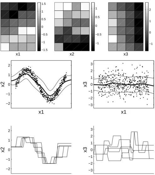
An example of using the conditional distributions is shown in fig. 7. The neighborhood width was chosen based on the maximum likelihood of test data. The data is three dimensional; there is a dependence between two
−1.5 −1 −0.5 0 0.5 1 1.5 x1 −1 −0.5 0 0.5 1 x2 −1 0 1 2 x3 −2 −1 0 1 2
x1
x2
−3 −2 −1 0 1 2 3x1
x3
−2 −1 0 1 2x1
x2
−3 −2 −1 0 1 2 3x1
x3
Fig. 7. Example of the use of SOM for data analysis. Top: all three component levels of a SOM trained down to optimal neighborhood width 0.2. Mid row: Training data and the means and standard deviations of the conditional densitiesp(x2|x1) and p(x3|x1) , integrated overx3 and x2, respectively. Bottom: nearest neighbor estimates based on the best matching units using five different values for x3 and x2, respectively.
of the variables, and one is independent, as follows: x2 = sin(ωx1) + #,
x3 ∼ N(0,1). This kind of a distribution can easily be modeled by means
of a two dimensional SOM; that is why no severe overfitting is observed and a small neighborhood width gives the best fit to test data. Yet it is not easy
to observe the dependence from the component level display. The conditional densities, on the other hand, are easy to interpret. Nearest neighbor regres sion also works relatively well, since the model complexity is correct.
By visual inspection of the map it is difficult to perceive the mean or shape of the conditional distributions and thus the reliability of the conclusions is practically impossible to assess. Choosing parameter values to optimize the density estimate may not result in a mapping that is also optimal for visual display. However, the examples shown in Figs. 5 and 6 indicate that this method will outperform any prefixed heuristic rule. In any case, the results of visual inspection should be validated by other, more reliable techniques.
6.1 Border effects
In typical implementations of the SOM, the neighborhood function is the same for each map unit. This causes problems near the borders of the map, where the neighborhood function gets clipped and thus becomes asymmetric. The effect is that, for no obvious reason, data samples which are outside the map are given less significance than those within the map. As a result, units close to the border have larger kernels and allow data points to reside farther away from the map units. Consequently, the border units are pulled towards the center of the map, and the map does not extend close to the edges of the input distribution until the neighborhood is relatively small and the regularization is loose. This leads to decrease of the likelihood for maps with large neighborhood (or increase of the quantization error), biasing the optimal width of the neighborhood towards smaller values.
This effect can be alleviated by normalizing the neighborhood function at the edges of the map. In the case of the sequential algorithm, it suffices to normalize the neighborhood function such that its sum is the same in each part of the map. When using the batch algorithm, the portion of the neigh borhood function that gets clipped off due to the finite size of the map lattice can be transferred to nearest edge units. Normalization of the neighborhood function is of particular importance, if the minimum distortion rule (4) is applied to winner selection. We see from Eq. 10 that when the sum of the neighborhood function is constant throughout the map, all cells have equal noise variance.
In practice we find that the minimal distortion rule will produce very simi lar results as the original rule in terms of model selection. The equalization of the neighborhood volume near map borders smoothes out the density model somewhat, as it allows better fit for the data sample with larger neighbor hood, as can be seen from Fig. 8. Obviously, the continuous density model, with minimum distortion rule, is favorable in many respects.
Training data
Original rule
Normalized neighborhood Minimum distortion rule
Fig. 8. Effect of the minimum distortion training rule on the density model. The neighborhood width is the same σ = 2.8 for all the maps. (This value is larger than would be optimal, as the purpose of the figure is to highlight the differences between these cases.) Note also, how the density kernel positions do not coincide with the reference vector positions. Especially in the middle of the maps the kernels are shifted upwards from the unit positions, according to Eq. 9. The jaggedness of the Voronoi cell boudaries is due to the discrete grid where the density is evaluated.
7
Conclusions
We have presented the probability density model associated with the SOM al gorithm. Also we have discussed some difficulties that arise in the application of the SOM to statistical data analysis. We have shown how the probability density model can be used to find the maximum likelihood estimate for the SOM parameters, in order to optimize the generalization of the model to new data. The parameter search involves a considerable increase in the computa tional cost, but in serious data analysis, the major concern is the reliability of the conclusions.
It should be stressed that although the density model is based on the error function which is not defined in all cases, in practice the only restriction in the application of the density function to data analysis is that the algorithm should be allowed to converge. Unfortunately, maximizing the likelihood of
data is not directly related with ensuring the reliability of the visual repre sentation of the SOM. Especially when the data dimension is high, the units that code the co-occurrences of all correlated variables cannot be grouped together on the map, and thus the conditional densities become distributed around the map. Such effects cannot be observed by visual inspection of the component levels, no matter how the model hyperparameters are set. Those effects can be revealed, to some extent, by calculating the conditional densities, or the conditional means and the confidence intervals.
The association of a generative probability density model with the SOM enables comparison of the SOM and other similar methods, like the Gen erative Topographic Mapping. If the theoretical difficulties of the SOM are avoided by adopting the minimum distortion winner selection rule, the main difference that remains is the hard vs. soft assignment of data to the units. The hard assignments of the SOM are perhaps easier to interpret and visu alize. In the SOM the activation of the units (ie., the posterior probability of the kernels given one data point) is always one for the winning unit and zero for the others, or a unimodal activation bubble of the shape of the neighbor hood around the winning unit, depending on the interpretation. With soft assignments the posterior probability may be multimodal (when two distant regions in the latent space are folded close to each other in the input space), and thus the activation is more difficult to visualize. Note, however, that this multimodal response gives visual indication of the folding, which may also be valuable. Apparently, the choice of methods depends on the application goals, and in real data analysis it is reasonable to apply different methods to decrease the effect of artefacts of the methods.1
1 Matlabr routines for evaluating the SOM probability density are available at
[1] C. M. Bishop, M. Svensen, and C. K. I. Williams. GTM: a principled alternative to the self-organizing map. In C. von der Malsburg, W. von Seelen, J. C. Vorbruggen, and B. Sendhoff, editors,Artificial Neural Net works—ICANN 96. 1996 International Conference Proceedings, pages 165–70. Springer-Verlag, Berlin, Germany, 1996.
[2] Christopher M. Bishop. Neural Networks for Pattern Recognition. Ox ford University Press, 1995.
[3] Christopher M Bishop, Markus Svensen, and Christopher KI Williams. Developments of the generative topographic mapping. Neurocomputing, 21(1):203–224, 1998.
[4] M. Cottrell, P. Gaubert, P. Letremy, and P. Rousset. Analyzing and representing multidimensional quantitative and qualitative data : De mographic study of the Rhone valley. the domestic consumption of the canadian families. In E. Oja and S. Kaski, editors, Kohonen Maps, pages 1–14. Elsevier, Amsterdam, 1999.
[5] Ed Erwin, Klaus Obermayer, and Klaus Schulten. Self-organizing maps: Ordering, convergence properties and energy functions. Biol. Cyb., 67(1):47–55, 1992.
[6] Tom Heskes. Energy functions for self-organizing maps. In Erkki Oja and Samuel Kaski, editors, Kohonen maps, pages 303–315. Elsevier, 1999.
[7] Teuvo Kohonen. Self-organizing formation of topologically correct fea ture maps. Biol. Cyb., 43(1):59–69, 1982.
[8] Teuvo Kohonen. Self-Organizing Maps, volume 30 of Springer Series in Information Sciences. Springer, Berlin, Heidelberg, 1995. (Second Extended Edition 1997).
[9] Jouko Lampinen and Timo Kostiainen. Overtraining and model selec tion with the self-organizing map. InProc. IJCNN’99, Washington, DC, USA, July 1999.
[10] Jouko Lampinen and Aki Vehtari. Bayesian approach for neural net works – review and case studies. Neural Networks, 2001. (Invited arti cle). To appear.
[11] Stephen P. Luttrell. Code vector density in topographic mappings: scalar case. IEEE Trans. on Neural Networks, 2(4):427–436, July 1991. [12] E. Oja and S. Kaski. Kohonen Maps. Elsevier, Amsterdam, 1999. [13] H. Ritter and K. Schulten. Kohonen self-organizing maps: exploring their
computational capabilities. InProc. ICNN’88 International Conference on Neural Networks, volume I, pages 109–116, Piscataway, NJ, 1988. IEEE Service Center.
[14] Michael E. Tipping and Christopher M. Bishop. Mixtures of principal component analysers. Technical report, Aston University, Birmingham B4 7ET, U.K., 1997.
[15] Akio Utsugi. Hyperparameter selection for self-organizing maps. Neural Computation, 9(3):623–635, 1997.
[16] Thomas Villmann, Ralf Der, Michael Herrmann, and Thomas M Mar tinetz. Topology preservation in self-organizing feature maps: exact definition and measurement. IEEE Transactions on Neural Networks, 8(2):256–266, 1997.
[17] Irma Welling, Erkki Kähkönen, Marjaana Lahtinen, Kari Salmi, Jouko Lampinen, and Timo Kostiainen. Modelling of occupants’ subjective responses and indoor air quality in office buildings. In Proceedings of the Ventilation 2000, 6th International Symposium on Ventilation for Contaminant Control, volume 2, pages 45–49, Helsinki, Finland, June 2000.
A
APPENDIX: Accuracy of the MCMC method
In the algorithm described in Section 5 one picks Lsamples and computes S, the number of samples that satisfy a certain condition. The task is to estimateq, the probability of a single sample satisfying the condition, based onS andL.S follows the binomial distribution
p(S|q, L) =qS(1−q)L−S (15) In Bayesian terms, the posterior distribution of qfor givenS andLis
p(q|S, L) = p(S|q, L)p(q) p(S|q, L)p(q)dq =
qS(1−q)L−S
qS(1−q)L−Sdq, (16) where the prior distributionp(q) is uniform. The integral in the denominator yields qS(1−q)L−Sdq= L−S k=0 (−1)k S+k+ 1 L−S k . (17)
Moments of the posterior can be written as serial expressions, for example
E(q) = qp(q|S, L)dq = L−S k=0 (−1) k S+k+2 L−S k L−S k=0 (−1) k S+k+1 L−S k , (18) and from the first and second moments we can derive an expression for the variance of the estimate ˆq=E(q). Unfortunately, the computation easily runs into numerical difficulties due to the alternating sign (−1)k. Exact values of
the binomial coefficients are required, and these can be difficult to obtain if, say, L >100.
To consider an approximation to the variance, observe that whenS =L the formulas simplify considerably and the variance can be written as
ν0=V ar(ˆq|S={0, L}) = L+ 1
(L+ 3) (L+ 2)2. (19) This is the minimum value of the variance for given L. The variance of the binomial distribution at the maximum likelihood estimate qml = S/L equals qml(1−qml)/L. We can combine these results to get a fairly good approximation
V ar(ˆq)≈ν∗(ˆq, L) =ν0+ ˆq(1−qˆ)/L, (20)
which slightly over-estimates the variance. A more precise approximation can be obtained directly from Eq. 16 by numerical integration. Picking Monte Carlo samples from the distribution N[ˆq,ν∗(ˆq)] truncated to the range [0,1] produces good results, except maybe at the very edges of the range, but there the exact valueν0 can be applied.
Let us write the sum in Eq. 12 asF =wiqi, wherewi =e(−βWb)(2πs2i)(d/2). The relative standard error of an estimate ofF equals
#= +Fˆ ˆ F = wi+qˆi wiqˆi = wi V ar(ˆqi) wiqˆi (21) Hence, to achieve a given accuracy #, Lshould be increased until
wi V ar(ˆqi) wiqˆi < #. (22)