Birth order and child outcomes: does maternal quality time matter?

(1)

Birth order and child outcomes:

does maternal quality time matter?

Chiara Monfardini

Sarah Grace See

(2)

Birth order and child outcomes:

does maternal quality time matter?

∗

Chiara Monfardini

†

and Sarah Grace See

‡

March 2012

Abstract

Higher birth order positions are often associated with poorer outcomes, possibly due to fewer resources received within the household. Using a sample of PSID-CDS children, we investigate whether the birth order effects in their outcomes are due to unequal allocation of the particular resource represented by maternal quality time. OLS regressions show that the negative birth order effects on various test scores are only slightly diminished when maternal time is included among the regressors. This result is confirmed when we account for unobserved heterogeneity at the household level, exploiting the presence of siblings in the data. Our evidence therefore suggests that birth order effects are not due to differences in maternal quality time received.

KeywordsBirth order; Achievement production ; Time use

JEL ClassificationD13, J12, J13, J22, J24

∗_{We thank Daniela Del Boca, Paul Frijters, Andrea Ichino, Cheti Nicoletti, and Maria Rita Testa; participants} in the departmental seminar in the University of Bologna, 6th Labour Markets and Demographic Change, 25th Annual Conference of the European Society for Population Economics, 2nd International Workshop on Applied Economics of Education, 52nd Anual Conference of Italian Economic Association, 36th Symposium of the Span-ish Economic Assocation, and the 7th PhD Presentation Meeting with the Royal Economic Society for helpful comments and suggestions.

†_{Department of Economics, University of Bologna, CHILD Torino, and IZA Bonn, Piazza Scaravilli 2, 40126} Bologna, Italy. email: chiara.monfardini@unibo.it. Corresponding author.

(3)

1 Introduction

Inequalities among individual outcomes have recently been examined in line with the evolu-tion of household condievolu-tions, as family sizes become smaller, and as more women enter the labor force and decide to bear children at later years. A growing literature investigates the link between family size and birth order on the one side, and inequalities in achievements and outcomes on the other side. Though pioneer studies fall under the fields of psychology and sociology, economic research is rapidly catching up, focusing on education and income out-comes, among others. Results predominantly show that individuals from larger family sizes have lower adult educational attainment and earnings (Black, Devereux, and Salvanes 2005; Gary-Bobo, Prieto, and Picard 2006; Sandberg and Rafail 2007), since family resources have to be divided among a greater number of offspring. And because those of higher birth order positions are born into larger family sizes, they are likewise found to have worse outcomes than those of lower birth order positions (Kantarevic and Mechoulan 2005).

A possible link between birth order and children outcomes may lie on parental investments on their children. Successfully establishing the existence of this link may not only provide a possible answer to overcome birth order effects, if present, but also lend a better explanation to the mechanism of intergenerational transmission. Financial, material, and time resources may be considered as investments into the child “quality” production (Becker 1974). Parental investments on their children, in turn, not only differ according to family finances and parental characteristics such as educational attainment, but also according to child-specific character-istics such as gender, birth order position, and number of children born in the family. For instance, a larger family size leads to smaller share of resources per child, given that family resources have to be divided among a greater number of children, assuming parents aspire to provide equally among their children. Birth order effects could favor the children with lower birth order positions essentially because they were born earlier and have received more re-sources from the parents.

Among the resources allocated by parents to children, time investment, and particularly that of the mother, is believed to be a crucial factor that contributes to the improvement of child educational and human capital outcomes. In the framework of the analysis of the intra-household allocation of resources, Price (2008) showed that while parents provide roughly equal time to each child at a given point in time, “birth order effects” come about due to the decreasing time that parents spend with their children as both get older. The result is that first-born children receive more cumulative quality time from the parents as compared to their second-born counterparts. This brings forth the argument that birth order effects in children outcomes may be due to differences in time resources received from parents.

This paper provides the first empirical assessment of the above argument. Do “birth order effects” mask differences in parental quality time received by the child? To answer this question we bridge two streams of literature: that on the child production function and that on the intrahousehold allocation of resources, and use data from the Child Development Supplement (CDS) of the Panel Study of Income Dynamics (PSID).This supplement contains a longitudinal survey on socio-economic conditions of interviewed families and individuals. It includes a time diary that contains information on how children spend their time on a representative weekday and weekend, how long they do certain activities, and with whom, including their parents. We focus on maternal time, in line with the emphasis of the existing literature, but check that findings for paternal time are similar.

(4)

Our results, in line with the literature, show a negative relationship between child cognitive test scores and birth order. We also find a negative relationship between maternal quality time and birth order, similar to Price (2008). However, the explanation for this pattern does not seem to rest on equity heuristic, since mothers are found to provide unequal time allocation to children of different birth order positions at each point in time. To test whether the birth order effect is also capturing different allocation of time resources, birth order and maternal time are both inserted as regressors in a child outcome equation. Ordinary least squares regression results show significant negative birth order effects and positive maternal time effects, with the magnitude of the birth order coefficients slightly diminished with the inclusion of maternal time. Once unobserved household-specific heterogeneity is controlled for with a sibling dif-ference approach, the coefficients of the birth order variables remain negative and statistically significant (and maternal quality time loses its significance). We therefore conclude that “birth order effects” do not mask differences in maternal quality time received.

The paper is organized as follows. Section 2 presents existing evidence for birth order ef-fects. Section 3 describes the data source and variables used. Section 4 illustrates the methodol-ogy, while section 5 discuses the descriptive and empirical results. Lastly, Section 6 concludes.

2 Background

Research on the child production function, initially developed by Becker and Tomes (1976), looks at child outcomes as resulting from a combination of inputs such as material/financial and time. More inputs invested will produce children with better achievements. In empirical studies, material and financial inputs have for a long time been proxied by family income and parental education, while attempts on considering the temporal resources have started out with the usage of proxies such as parental employment and weekly work hours (Bernal 2008; Todd and Wolpin 2003; Blau and Grossberg 1992). More recently, availability of time diaries data has brought in a significant improvement in the analysis of time inputs. The proxy variables indeed represent a measure of the maximum amount of time not spent with children, since non-working time of parents are not necessarily and entirely used together with their children. Time diaries, on the other hand, provide the amount of time that parents are actually with their children, as well as information on the activities performed together. A limited literature has recently looked at time inputs as determinants of child outcomes, mostly using the PSID-CDS. Hsin (2007) examines how different measures of maternal care (i.e. total quantity, engaged, quality time) affect children’s test scores. She found within an OLS approach that more time spent with mothers has a positive effect on the verbal skills of the children, but only for the children whose mothers have high verbal abilities. Applying a generalized propensity score, Carneiro and Rodrigues (2009) concluded that more time spent with mothers leads to better cognitive test outcomes of the children, at least for the younger ones. Meanwhile, Del Boca, Flinn, and Wiswall (2010) estimated a structural model of the cognitive developmental process of the children, nested within the life cycle behavior of the household, and showed that parental active time is a productive input for young children, though with declining effect.

Existing literature on the so-called “birth order effects” has for a long time been prevalent in the field of psychology (Kidwell 1981; Sulloway 2007; Zajonc 1976). Here, differences in outcomes such as intellectual attainments and personalities are explained either by the differing intellectual environments experienced by the children in the so-called confluence model

(5)

(Za-jonc 1976), or by the distinct roles that each child plays in the family, as suggested in the family dynamics model (Sulloway 2007). Adoption into the field of economics remains relatively new, and focuses mainly on inequalities in human capital and labor market outcomes measured in terms of educational attainment (Blake 1981; Black, Devereux, and Salvanes 2005; Booth and Kee 2009; Kantarevic and Mechoulan 2005), test scores (Blake 1981; Conley, Pfeiffer, and Velez 2007; Leibowitz 1974), and income earnings (Behrman and Taubman 1986; Kantarevic and Mechoulan 2005). Although there are some studies that claim little or no birth order effect (e.g. Hauser and Sewell 1985), most empirical findings in the economic literature show neg-ative or U-shaped results (Hanushek 1992). Among those that looked at birth order effects in educational outcomes, Heiland (2009) found that U.S. first-borns of the 1979 cohort of National Longitudinal Survey of Youth (NLSY79) have higher scores in the Peabody Picture Vocabulary Test-Revised (PPVT-R), a standardized test of early verbal ability. Kantarevic and Mechoulan (2005) used a PSID sample and claimed that a “first-born advantage” in terms of educational attainment is already evident as early as high school age, and it persists until the professional life as measured by income earnings. Conley, Pfeiffer, and Velez (2007) found within a PSID-CDS children sample that first-borns generally perform better in Woodcock-Johnson Revised (WJ-R) Tests of Achievement than their younger siblings. Meanwhile, Black, Devereux, and Salvanes (2007) found that lower birth order children have higher scores in intellectual quotient on a Norwegian sample. All the above-mentioned studies exploit the presence of sibilings in the data and adopt family fixed effect estimation to identify birth order effects net of unobserved confounders at the household level.

The negative relationship between birth order and outcomes is explained by the mechanism of resource allocation within the household. Maintaining the assumption that provision of greater resources improves children outcomes, a family with a greater number of children lets each child receive a smaller share of the family resources, as compared to a child born in a smaller family (Becker 1974; Becker and Tomes 1976). As higher birth order children are more likely to be born in bigger families, a latter-born child will also receive fewer resources, since the resources have already been previously allocated to the earlier-born children. Becker and Lewis (1973) proposed a quantity-quality trade-off in the family, saying that larger family sizes produce lower “quality” children since more people have to share the available resources. Siblings with a smaller age gap also are exposed to sibling competition for parental resources more than siblings with a larger age gap, hence the former are more likely to receive less resources and experience birth order effects. Even if parents decide to allocate resources more equally among the children, the result still creates a cumulative inequality. This is the so-called equity heuristic model proposed by Hertwig, Davis, and Sulloway (2002). Compared to the first-borns who enjoy being the “only child” when the younger siblings have not been born, and the last-born children who become the “only child” when the older siblings leave the household, middle-born children never have the opportunity of being the “only child” in the family. As such, middle-born children always share the parental resources with other siblings and always receive lesser cumulative shares of the resources. Unlike the earlier-born children, latter-born children experience a poorer resource environment, such as less parental time during the child’s early years. One reason for birth order effects within the equity heuristic framework is that they may be more of a function of perception than actual, such that children perceive themselves as being treated unequally, even though they are treated equally. Parents may also have a different definition of “equality” from the children’s. Nevertheless, the equity heuristic explanation shows that birth order effects may occur even though parents aim to be equal at

(6)

all times. With a neighbor-matching estimation that allows for the comparison of first-borns and second-borns from similar two-children households of American Time Use Survey (ATUS) respondents, Price (2008) found that parents provide approximately equal amounts of quality time to their children at each point in time, but spend less time with each child as they both get older, resulting in less cumulative parental quality time by second-born children.

3 Data

Our empirical strategy relies on both streams of literature described above. Exploiting informa-tion on both children time use and test scores contained in the Child Development Supplement (CDS) of the Panel Study of Income Dynamics (PSID), we are able to estimate birth order effects in a child outcome equation with or without conditioning for parental time.

The Panel Study of Income Dynamics is primarily sponsored by the National Science Foun-dation, the National Institute of Aging, and the National Institute of Child Health and Human Development and is conducted by the University of Michigan. The study is a longitudinal data of United States individuals, with information regarding their economic, demographic, socio-logical, and psychological status and well-being. The interview started in 1968, with the initial sample of 4,800 families coming from a cross-sectional national sample drawn by the Survey Research Center (SRC) and a national sample of low-income families from the Survey of Eco-nomic Opportunity (SEO) conducted by the Bureau of the Census for the Office of EcoEco-nomic Opportunity. The succeeding interviews followed the original sample through the years. As of 2001, there are more than 7,000 interview families in the dataset. The latest available wave of the PSID is of year 2007.

The CDS dataset was funded by the National Institute of Child Health and National De-velopment (NICHD), with the first interview in 1997. The second wave is in 2002/03, and the third is in 2007. The CDS-I contains 3,563 children of 0 to 12 years old belonging to 2,394 families (88%). The CDS-II successfully re-interviewed 2,907 children from 2,019 families (91%), with ages 5 to 18, while the CDS-III has 1,506 children (90%) re-interviews, of 10 to 19 years old. Children from the original sample of 18 years or above are included in the Transition into Adulthood (TA) dataset. The CDS looks into the human capital development of the interviewed children, with measures such as home environment, family processes, time diaries, school environment, and measures of cognitive, emotional, and physical performance. Information for up to two randomly-chosen children in a family are available. The time di-aries contain the activities performed by each child on a weekday and a weekend, how long the activities were performed, and with whom. Cognitive measurements concern verbal and mathematical skills. A subjective non-cognitive measure of behavioral problem index (BPI) is also available, which includes information on mood swings, aggression, etc.

The analysis uses a pooled sample consisting of 533 PSID-CDS sibling-pair children (1066 children) from 5 to 18 years old, with the average at 12 years, who are living in intact families1 of two to five children.

(7)

3.1 Outcome Measures

The achievements explored in our analysis are three cognitive outcomes in age-standardized and raw formats and one non-cognitive outcome in raw format. The cognitive measures are test components in the Woodcock Johnson Revised (WJ-R) Test of Achievement. Raw scores are essentially the number of items completed in the test, while the standardized scores are obtained standardizing the raw scores according to the respondent’s age2_{. Verbal outcomes}

are measured by the letter word and passage comprehension test components. The letter word test assessment measures symbolic learning (matching pictures with words) and reading iden-tification skills (identifying letters and words). It starts from the easiest items (ideniden-tification of letters and pronunciation of simple words), progressing to the more difficult items, such that college students and adults would start on a different item than do pre-school children. The passage comprehension assessment measures comprehension and vocabulary skills using multiple-choice and fill-in-the-blank formats. The applied problem test measures mathematical skill in analyzing and solving practical problems in mathematics. The non-cognitive outcome is a behavioral problem index measuring the incidence and severity of child behavior problems, according to the responses of the primary caregiver. While there are two components to the index, externalizing and internalizing, only the total raw score is considered here.

3.2 Parental Time

We rely on a direct measure of maternal time with children. The availability of time diaries represents a significant advantage with respect to proxies such as employment status or weekly worked hours. Indeed, the latter has been found to have ambiguous effects on children out-comes (Blau and Grossberg 1992; James-Burdumy 2005), since maternal non-working time is not necessarily entirely spent with the children.3

The PSID-CDS provides detailed information on children’s time use on a random represen-tative weekday and a random represenrepresen-tative weekend. Information is available for up to two children in a family, specifying the type of activity performed, the amount of time spent on each activity over a 24-hour period, and the company involved in performing the activity (i.e. ’Who was doing this activity with the child?’, ’Who (else) was there but not directly involved in the activity?’). Parental time is believed to be a crucial input for a child’s outcome and various definitions and measurements have been considered in the existing literature, e.g. Hsin (2007) looked at time in terms of total quantity, active engagement, and selected activities. Although both parental times are important in the child’s development process, the literature has empha-sized the role of maternal time, largely due to the increasing incidence of maternal employment that serves as a trade-off for child care time. Therefore, we refer to maternal time throughout the analysis, but we conduct a parallel analysis using paternal time4_{. For the sake of}

compa-rability, specific activities performed with the parents are selected to replicate a “quality time”

2_{The age standardization process allows for comparison of children of the same age, eliminating the}

discrep-ancy in the results due to different ages.

3_{For instance, employed mothers may compensate for work hours by spending more of their available time}

with their children and less time on other activities such as leisure (Huston and Aronson 2005).

4_{Analysis of paternal time uses information with respect to fathers, i.e. birth order and number of children}

according to the father. Results are available upon request. Meanwhile, a specification of combining both parents is problematic, as information from the parents may not coincide, e.g. a child can be considered a second-born from the mother, but a first-born from the father.

(8)

aggregate as defined by Price (2008). “Quality time” is composed of activities that the children perform with each parent, in which either the child was the primary focus of the activity or there was a reasonable amount of interaction.

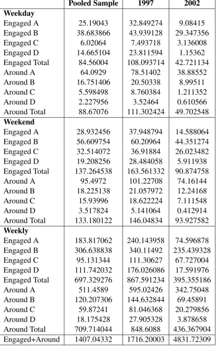
Table 1 lists the categories of activities as defined by Price (2008), as well as the average minutes spent on each category on a representative weekday and on a representative weekend, and whether the mother is actively engaged or just around while the child was doing the ac-tivity. Quality time is categorized into four, with each category including specific activities. Category A includes reading, playing, doing homework, talking, teaching, and doing arts and crafts. Category B is eating, while Category C are playing sports, attending performing arts, and participating in religious practices. Category D refers to looking after and physical care. The total averages indicate that a mother spends more time being around the child on a weekday than being actively engaged. This is particularly true for Category A activities. Comparing the average minutes by activity categories, a mother spends more time actively engaged with the child doing all the rest of the quality time activities (Categories B to D). We also see lower av-erages in the 2002 wave than in the 1997 wave, which is likely due to the aging process. When aggregated into a weekly measure by multiplying the weekday amount by five, multiplying the weekend amount by two, and getting the summation of the two products, lagged maternal quality time for the pooled sample averages at 1,407 minutes, and averages at 1,716 and 831 minutes for 1997 and 2002, respectively. For ease of interpretation, quality time is aggregated into an hourly weekly measure.

(Insert table 1 here)

4 Empirical Strategy

4.1 Birth Order and Maternal Quality Time

In order to test whether “birth order effects” in children outcomes are coursed through maternal quality time, we first establish the relationship between birth order and maternal quality time running the following OLS regression:

T imeijt =β0+β1BOi+β2F Sj+β3T2t+β4Xijt+β5Xi+β6Zj +ijt (1) The dependent variableT imeijt stands for the quality time a childiborn in familyj receives from the mother observed at each period t; T2t is a dummy variable that indicates the period of observation (i.e. 2007 versus 2002); BOi is a set of dummy variables indicating the birth order position of the child;F Sjis the set of dummy variables indicating the number of children born to the parent;Xijtis a vector of child- and household-specific time-varying characteristics such as the child’s age; Xi stands for the observable individual variables such as child’s birth weight, race, gender, and maternal childbirth age; and Zj is a vector of household-specific characteristics including parental years of education, and parental employment status.

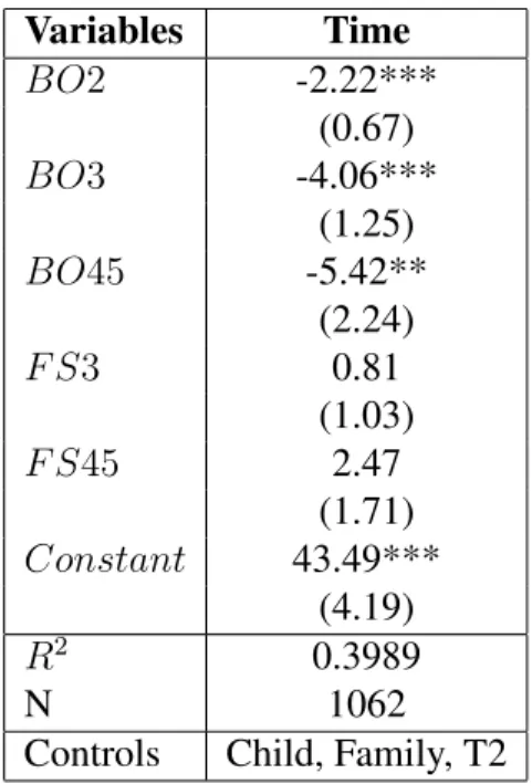
OLS results contained in Table 2 show a negative and significant relationship between birth order and maternal quality time, with the magnitudes increasing with higher birth order posi-tions. At the same age, higher birth order children receive less time as compared to their first-born counterparts. Second-first-born children receive a relative average of 2.22 hours per week less maternal quality time, third-born children receive 4.06 weekly hours less than their first-born

(9)

counterparts, while fourth-born and fifth-born children receive 5.42 weekly hours less. The family size dummy variables, although positive, are not statistically significant. These results are consistent with the evidence in Price (2008). However, we find that a negative birth order pattern exists in the parental time received by the child at each age (not only in the cumulative amount of time received at each period).

(Insert table 2 here

4.2 The Child Outcome Equation

The results of the previous section show that children with higher birth order positions receive less maternal quality time at each age, and provides evidence of inequality in the intrahouse-hold allocation of resources. In order to spot the role of the particular resource represented by maternal quality time in determining birth order effects, we adopt a reduced-form child pro-duction function model, in which past and current child and family characteristics, and input measures, produce the child test score output (see Todd and Wolpin, 2007). Birth order vari-ables are inserted on the right-hand side of the equation, together with the quality time input in a “horse race” regression to test for the extent to which time input explains the birth order effects. Due to a small sample size, the model is estimated pooling the two years of observation (2002, 2007).

T estijt=γ0+γ1BOF Si +γ3T imeit−1+γ4T2t+γ5Xijt+γ6Xi+γ7Zj +ijt (2) The dependent variableT estijtstands for the different test outcomes observed at each pe-riodtof a childiborn in familyj, and include letter word (LW), passage comprehension (PC), applied problem (AP), and behavioral problem index (BPI).BOF Siis the family-specific birth order position of a child in his own family. This specification differentiates the birth order ef-fect by family size. For instance, a second-born of a 2-children family is differentiated from the second-borns of the 3-children and of the 4-to-5-children families. The time input is measured as the maternal quality time received at the previous period, T imeit−1. We prefer this lagged measurement over the contemporaneous one, in order to mitigate the simultaneity issue that arises when a contemporaneous outcome is regressed on a contemporaneous input. The child and family characteristics we insert as control,Xijt, Xi, Zj have already been defined above. Birth weight is likely to be highly correlated with family size and birth order5. Male children generally have lower verbal and reading achievement test scores, hence an expected negative correlation with letter word and with passage comprehension test scores. Non-white children are also expected to score lower than white children6.

A parallel specification considers instead independent effects of birth order position (BOi) and family size (F Si):

T estijt=β0+β1BOi+β2F Sj+β3T imeit−1+β4T2t+β5Xijt+β6Xi+β7Zj+ijt (3)

5_{For instance, a latter-born child from a larger family size will more likely have a lower birth weight due to}

being born to an older mother (Rosenzweig and Zhang 2009).

6_{Family income is not included as a regressor, because of a sample size issue due to a significant number of}

(10)

In both models,ijtis thought of as a three-way errror component:

ijt =αi +ψj(t)+ρijt

including a child-specific time-constant unobserved heterogeneity term (αi), a household-specific unobserved heterogeneity component that is possibly time-varying (ψj(t)), and an idiosyncratic error (ρijt).

We estimate the birth order and time use variable effects,γ1 andγ3in model (2) (β1 andβ3 in model (3)), with the following approaches:

1. Pooled OLS, which provides consistent estimates of the above coefficients of interest

only under the assumption that all the right-hand side variables, including the inputs, are orthogonal toαiandψj(t)

2. Sibling Difference, which is useful to identify birth order and time use variable effects

net of unobserved family-specific components, possibly correlated with the observed re-gressors, under the assumption of time-constant family unobserved heterogeneity, i.e.

ψj(t)=ψj;

∆jT estit=γ1∆jBOF Si+γ3∆jT imeit−1+γ4∆jT2t+γ5∆jXijt+γ6∆jXi+ ∆jijt (2a) ∆jT estit=β1∆jBOi+β3∆jT imeit−1+β4∆jT2t+β5∆jXijt+β6∆jXi+∆jijt; (3a) In order to implement this estimation strategy, the sibling difference is taken at each time period (2002, 2007), before the pooling of the two years of observations.

5 Results

5.1 Descriptive Analysis

5.1.1 The Sample

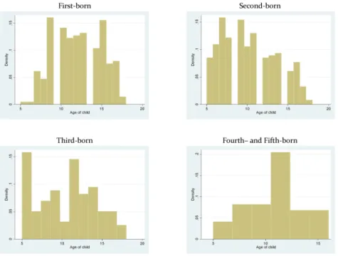
The summary statistics of the relevant variables in our sample are shown in Table 3. Half of the sample are males, and 18% are Blacks. First-born children occupy 36% of the sample, second-borns comprise 43%, third-borns are 17%, and 4th- and 5th-borns are 5%. Meanwhile, the pooled sample has an average of 2.8 children in the family. Almost half of the sample are 2-children families, at 42%; 41% are 3-children families, 17% are families with 4 to 5 children. The distribution of ages by birth order positions are in the graphs in the Appendix, showing that the sample contains variation in ages in each birth order position, an important requirement not to confuse birth order effects for age effects.

The letter word standardized score of the pooled sample averages at 106.73 with a standard deviation of 16.90 points, while the raw test score averages at 44.69, with a standard deviation of 8.46 points. The sample average of the passage comprehension standardized score is at 105.66, with a standard deviation of 15.40 points, while the raw score averages at 26.26, with a standard deviation of 6.76. Applied problem averages at 107.20 and 38.14 for standardized and raw, with standard deviations of 15.97 and 8.11, respectively. The behavioral problem index averages at 13.87, with a standard deviation of 11.02.

(11)

5.1.2 Within Family Variation

If the observed outcome of each child in a family is thought of as including an error term with individual-specific and family-specific components, the variance of this term can be decom-posed into between-family and within-family variations. The sibling correlation coefficients of the test scores and maternal quality time for interviewed sibling pairs shown in Table 4 corre-spond to the share of variance that is attributable to the family background effects. The higher the sibling correlation coefficients, the higher is the share of the variance that is due to the family-specific components. The sibling correlations for the standardized cognitive test scores are approximately between 0.45 to 0.55, while that for the behavioral problem index is at 0.09. That for maternal quality times are at 0.35 and 0.28 for lagged and contemporaneous, respec-tively. This provides evidence on the existence of variation within the family on which we base our identification strategy.

5.1.3 Child Outcomes and Birth Order

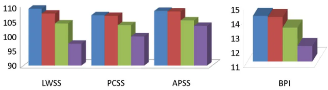
Figure 1 exhibits the average test scores for each birth order position, with a decreasing pat-tern of average cognitive test scores for each higher birth order position. The patpat-tern for the non-cognitive test score shows a positive birth order effect; however, birth order effects for the behavioral problem index are expected to be inconclusive because of the nature of its measure-ment. Unlike the cognitive test scores, which are objectively evaluated, the behavioral problem index is derived from a subjective evaluation of the child’s behavior by the primary caregiver.

(Insert figure 1 here)

5.1.4 Child Outcomes and Maternal Quality Time

Table 5 shows the average standardized test scores by the amount of maternal quality time received. The sample is divided into two groups, based on the average quality time of the sample: those who received less than the average quality time and those who received greater than or equal to the average time in the pooled sample. It is evident that receipt of maternal quality time greater than the average is associated with better performance in the test outcomes. The differences are statistically significant, as shown by the mean comparison tests.

5.2 Does Maternal Quality Time Explain Birth Order Effects?

We provide in this section the results on the estimated child outcome equation. We take as dependent variable both the standardized and the raw test scores. The latter is a reasonable measure once we control for age in our regressions. The first set of results is obtained using the OLS, with standard errors corrected for the correlation of error terms among siblings.

Tables 6 to 9 show the estimation results for the four outcomes for our preferred model of specification (2), i.e. using family-specific birth order effects, with the first-borns as the benchmark. Results for model (3), i.e. using straightforward birth order positions of each child,

(12)

are available upon request. Each column shows the result for a different model estimation approach. The first two columns contains standard pooled OLS coefficients on interviewed sibling pairs, excluding and including lagged maternal quality time. These are comparable to the sibling difference approach on the next two columns, again excluding and including maternal quality time. We report regressions for the Behavioral Problem Index for the sake of completeness, but are aware that the interpretation requires some caution, since it is a self-reported measure. Moreover, such a non-cognitive outcome may require a different production function to that of cognitive outcomes considered in our analysis.

(Insert tables 6 to 9 here)

The pooled OLS birth order estimated effects exhibit statistically significant negative pat-terns, with the magnitudes increasing for each higher birth order position of each family size. For instance, the second-born of a two-children family scores 3.79 points less in the letter word standardized test than a first-born child of any family size does, a difference of less than one-fourth of a standard deviation. The maternal quality time shows a positive and statistically significant coefficient only for the letter word outcome, and decreases the magnitudes of the negative birth order variables. Likewise, the magnitudes of the negative birth order effects are “bloated” when maternal quality time is not accounted for. The non-cognitive outcome shows some significance for some birth order positions of family sizes of 3 or more children. This suggests that children from larger families have more behavioral problems.

OLS estimations are however criticized to provide biased estimates. With respect to birth order and family size, unmeasured parental endowments and family size preferences are po-tential sources of unobserved heterogeneity affecting child development outcomes. If parents with below-average resources also have fewer children, then children with lower birth order positions are more likely to have poorer outcomes compared to their higher birth order counter-parts. The opposite is also true, if parents with above-average resources prefer to have children of better abilities by foregoing a larger family size. The sibling difference approach allows us to control for unobserved household-specific characteristics that may contribute to the above-mentioned bias. The results again show a general negative and increasing magnitude pattern for the birth order variables, particularly for smaller family sizes and especially for the raw scores. Including the lagged maternal quality time within the sibling difference approach does not bring significant changes to the coefficients of the negative birth order variables. Notice also that once time-constant family-specific unobserved heterogeneity is contolled for, mater-nal quality time variable is no longer statistically significant, suggesting that matermater-nal quality is important as a family-level rather than an individual input. As far as the non-cognitive outcome is concerned, the sibling difference approach entails a positive coefficient for the latter-born of each family size, i.e. second-born of two-children; third-born of three-children; third-born, fourth- and fifth-born of four- to five-children families. This pattern suggests that the signifi-cance of the coefficients of the family-specific birth order variables in the pooled OLS is driven by confounding unobserved factors at the household level. Controlling for them reveals the un-derlying negative “birth order effects”, with higher birth order children having more behavioral problems. Similar to the findings for the cognitive outcomes, maternal time does not appear to be the channel through which birth order positions exert their effect7_.

7_{As a robustness check, specifications that use both lagged and contemporaneous maternal quality time were}

(13)

In summary, pooled OLS results show negative and statistically significant coefficients for the birth order variables, with the magnitudes slightly diminishing with the inclusion of the maternal quality time in the regression. The coefficients of birth order variables remain gen-erally negative and statistically significant when family heterogeneity is controlled for, (while maternal quality time loses its significance). We conclude therefore that birth order effects on children outcomes do not mask differences in maternal quality time received, as suggested by Price (2008). Although we confirm his finding about the existence of a negative birth order ef-fect in parental quality time, our evidence indicates that birth order position is likely to convey information about resources received by the child other than parental time.

6 Conclusions

Children of higher birth order positions are found to have poorer outcomes. Literature suggests that inequalities in children outcomes based on the respective birth order positions could be due to differences in resources received. This paper focuses on the role of a particular resource received from parents - maternal quality time. It investigates whether birth order effects in children outcomes are due to differences in quality time received, by looking at the relationship between children’s birth order position, maternal quality time input, and children’s cognitive and non-cognitive outcomes.

Using data from the Child Development Supplement of the Panel Study of Income Dynam-ics, we find a negative relationship between birth order and all the available test scores, which is consistent with the findings of Black, Devereux, and Salvanes (2005, 2007), Kantarevic and Mechoulan (2005), and Heiland (2009), among others. A negative relationship is also found between birth order and maternal quality time, partly consistent with Price (2008).

We estimate horse race regressions to test whether the birth order effects on children out-comes resists to the inclusion of maternal quality time among its determinants. Exploiting the presence of siblings in the data, we are able to remove potential bias arising from unobserved household-specific heterogeneity, and find negative and significant birth order effects for both cognitive and non-cognitive outcomes, with and without controlling for maternal quality time. These results suggest that maternal quality time is not the driving factor behind birth order ef-fects: to the extent that birth order effects are the outcome of the mechanism of intrahousehold allocation of resources, they must be explained by other resources differently allocated to each offspring.

estimation. As with the cases presented above, the coefficient loses its significance with the application of the sibling difference approach.

(14)

References

[1] Becker G (1974) A Theory of Social Interactions. Journal of Political Economy 82(6):1063-1093

[2] Becker G, Lewis H (1973) On the Interaction Between the Quantity and Quality of Chil-dren. Journal of Political Economy 81(2):S279-S288

[3] Becker G, Tomes N (1976) Child Endowments and the Quantity and Quality of Children. Journal of Political Economy 84:143-162

[4] Behrman J, Taubman P (1986) Birth Order, Schooling, and Earnings. Journal of Labor Economics 4(3):S121-S14

[5] Bernal R (2008) The Effect of Maternal Employment and Child Care on Children’s Cog-nitive Development. International Economic Review 49:1173-1209

[6] Black S, Devereux P, Salvanes S (2005) The More the Merrier? The Effect of Family Size and Birth Order on Children’s Education. Quarterly Journal of Economics 120(2):669-700.

[7] Black S, Devereux P, Salvanes K (2007) Older and Wiser? Birth Order and IQ of Young Men. NBER Working Papers 13237, National Bureau of Economic Research, Inc. [8] Blake J (1981) Family Size and the Quality of Children. Demography 18(4):421-442 [9] Blau F, Grossberg A (1992) Maternal Labor Supply and Children’s Cognitive

Develop-ment. Review of Economic Statistics 74(3):474-481

[10] Booth A, Kee HJ (2009) Birth Order Matters: The Effect of Family Size and Birth Order on Educational Attainment. Journal of Population Economics 22:367-397

[11] Carneiro P, Rodrigues M (2009) Evaluating the Effect of Maternal Time on Child Devel-opment Using the Generalized Propensity Score. Institute for the Study of Labor, 12th IZA European Summer School in Labor Economics

[12] Conley D, Pfeiffer K, Velez M (2007) Explaining Sibling Differences in Achievement and Behavioral Outcomes: The Importance of Within- and Between-Family Factors. Social Sciences Research 36:1087-1104

[13] Del Boca D, Flinn C, Wiswall M (2010) Household Choices and Child Development. Carlo Alberto Notebooks No. 149

[14] Gary-Bobo R, Prieto A, Picard N (2006) Birth Order and Sibship Sex Composition as In-struments in the Study of Education and Earnings. Centre for Economic Policy Research, CEPR Discussion Paper Series No. 5514

[15] Hanushek E (1992) The Trade-off Between Child Quantity and Quality. Journal of Polit-ical Economy 100:84-117

[16] Hauser R, Sewell W (1985) Birth Order and Educational Attainment in Full Sibships. American Educational Research Journal 22(1):1-23

(15)

[17] Heiland F (2009) Does the Birth Order Affect the Cognitive Development of a Child? Applied Economics 41(14):1799-1818

[18] Hertwig R, Davis J, Sulloway F (2002) Parental Investment: How an Equity Motive Can Produce Inequality. Psychological Bulletin 128(5):728-745

[19] Hsin A (2007) Mothers’ Time with Children and the Social Reproduction of Cognitive Skills, Working paper, California Center for Population Research Working Paper Series [20] Huston A, Aronson S (2005) Mother’s Time with Infant and Time in Employment as

Predictors of Mother-Child Relationships and Children’s Early Development. Child De-velopment 76(2):467-482

[21] James-Burdumy S (2005) The Effect of Maternal Labor Force Participatioin on Child Development. Journal of Labor Economics 23(1):177-211

[22] Kantarevic J, Mechoulan S (2005) Birth Order, Educational Attainment, and Earnings: An Investigation Using the PSID. Journal of Human Resources 41(4):755-776

[23] Kidwell J (1982) The Neglected Birth Order: Middleborns. Journal of Marriage and Fam-ily Issues 44:225-235

[24] Leibowitz A (1974) Home Investments in Children. Journal of Political Economy 82:111-131

[25] Panel Study of Income Dynamics, Child Development Supplement public use dataset. Produced and distributed by the University of Michigan with primary funding from the National Science Foundation, the National Institute of Aging, and the National Institute of Child Health and Human Development. Ann Arbor, MI.

[26] Price J (2008) Parent-Child Quality Time: Does Birth Order Matter? Journal of Human Resources 43(1):240-265

[27] Rosenzweig M, Zhang J (2009) Do Population Control Policies Induce More Human Capital Investment? Twins, Birth Weight and China’s “One Child” Policy. Review of Economic Studies 76:1149-1174

[28] Sandberg J, Rafail P (2007) Family Size, Children’s Cognitive Skills and Familial Inter-actions: U.S., 1997-2002. PAA Annual Meeting. New York, NY

[29] Sulloway F (2007) Birth Order and Intelligence. Science 1711-1712

[30] Sulloway F (2007) Chapter 21: Birth Order and Sibling Competition. In: Dunbar R, Barrett L (ed) The Oxford Handbook of Evolutionary Psychology, Oxford University Press 297-311

[31] Todd P, Wolpin K (2003) On the Specification and Estimation of the Production Function for Cognitive Achievement. Economic Journal 113(485):F3-F33

(16)

Table 1: Averages of Maternal Quality Time Activities in Minutes Pooled Sample 1997 2002 Weekday Engaged A 25.19043 32.849274 9.08415 Engaged B 38.683866 43.939128 29.347356 Engaged C 6.02064 7.493718 3.136008 Engaged D 14.665104 23.811594 1.15362 Engaged Total 84.56004 108.093714 42.721134 Around A 64.0929 78.51402 38.88552 Around B 16.751406 20.50338 8.99511 Around C 5.598498 8.760384 1.211352 Around D 2.227956 3.52464 0.610566 Around Total 88.67076 111.302424 49.702548 Weekend Engaged A 28.932456 37.948794 14.588064 Engaged B 56.609754 60.20964 44.351274 Engaged C 32.514072 36.91884 26.023482 Engaged D 19.208256 28.484058 5.911938 Engaged Total 137.264538 163.561332 90.874758 Around A 95.4972 101.22708 74.16144 Around B 18.225138 21.057972 12.24168 Around C 15.93996 18.622224 7.111548 Around D 3.517824 5.141064 0.412914 Around Total 133.180122 146.04834 93.927582 Weekly Engaged A 183.817062 240.143958 74.596878 Engaged B 306.638838 340.11492 235.439328 Engaged C 95.131344 111.30627 67.727004 Engaged D 111.742032 176.026086 17.591976 Engaged Total 697.329276 867.591234 395.355186 Around A 511.4589 595.02426 342.75048 Around B 120.207306 144.632844 69.45891 Around C 59.87241 81.046368 20.279856 Around D 18.175428 27.905328 3.878658 Around Total 709.714044 848.6088 436.367904 Engaged+Around 1407.04332 1716.20003 4831.72309

A=Reading; Playing, not sports; Helping with homework; Helping, Teaching; Arts and crafts; B=Meals; C=Playing sports; Attending performing arts; Participating in religious activities; D=Recipient of personal care; Organizing and planning; Attending events

(17)

Table 2: OLS Results for Maternal Quality Time Variables Time BO2 -2.22*** (0.67) BO3 -4.06*** (1.25) BO45 -5.42** (2.24) F S3 0.81 (1.03) F S45 2.47 (1.71) Constant 43.49*** (4.19) R2 _0.3989 N 1062

Controls Child, Family, T2

Pooled Sample. Child controls include child’s age, child’s age squared, birth weight, gender, dummy variable for black race. Family controls include mother’s age at childbirth, mother’s education level in years, and mother’s employment status. Standard errors are shown in parentheses, followed by indicators of significance levels (*** significant at 1% level, ** significant at 5% level, * significant at 10% level).

(18)

Table 3: Summary Statistics

Pooled Sample 2002 2007

Variables Mean Mean Mean

(Std.Dev.) (Std.Dev.) (Std.Dev.) Child’s age 11.60882 10.9723 13.17532

3.186809 3.350194 2.023101 Child’s gender (Male=1) 0.4943715 0.4868074 0.512987 Child’s race (Black=1) 0.1763602 0.176781 0.1753247 Child’s birth weight, pounds 7.108818 7.146438 7.016234

1.2853 1.247849 1.370844 Mother’s age at childbirth 28.20732 28.23219 28.1461

5.16354 5.006355 5.539443 Lagged maternal education in years 13.37523 13.35092 13.43506 2.516781 2.494023 2.575063 Lagged maternal employment status (employed=1) 0.6022514 0.5989446 0.6103896 1st-born (BO1) 0.3555347 0.3443272 0.3831169 2nd-born (BO2) 0.4333959 0.4261214 0.4512987 3rd-born (BO3) 0.1660413 0.176781 0.1396104 4th-5th born (BO45) 0.0450281 0.0527704 0.025974 2-children families (FS2) 0.424015 0.4195251 0.4350649 3-children families (FS3) 0.4071295 0.4010554 0.4220779 4-5 children families (FS45) 0.1688555 0.1794195 0.1428571 1st of 2 children (BO1FS2) 0.2120075 0.2097625 0.2175325 2nd of 2 children (BO2FS2) 0.2120075 0.2097625 0.2175325 1st of 3-children (BO1FS3) 0.1097561 0.1029024 0.1266234 2nd of 3-children (BO2FS3) 0.1772983 0.1728232 0.1883117 3rd of 3-children (BO3FS3) 0.120075 0.1253298 0.1071429 1st of 4-5 children (BO1FS45) 0.0337711 0.0316623 0.038961 2nd of 4-5 children(BO2FS45) 0.0440901 0.0435356 0.0454545 3rd of 4-5 children (BO3FS45) 0.0459662 0.0514512 0.0324675 4th-5th pf 4-5 children (BO45FS45) 0.0450281 0.0527704 0.025974 Letter word standardized score (LWSS) 106.7317 107.2586 105.4351 16.90235 17.30614 15.81733 Letter word raw score (LWRAW) 44.69137 43.50792 47.6039

8.458985 9.16713 5.388997 Passage comprehension standardized score (PCSS) 105.6604 107.2995 101.6266 15.39645 15.09831 15.40401 Passiage comprehension raw score (PCRAW) 26.2561 25.46966 28.19156 6.757857 7.193201 5.055296 Applied problem standardized score (APSS) 107.1979 107.1016 107.4351 15.97237 16.31514 15.11882 Applied problem raw score (APRAW) 38.13602 36.98945 40.95779 8.10861 8.47624 6.300419 Behavioral Problem Index (BPI) 13.86867 7.675462 29.11039 11.02237 6.01541 2.114204 Lagged maternal quality time (QualTt−1) 23.45072 26.67898 15.50584

14.69644 15.21806 9.442178 Number of observations 1066 758 308

(19)

Table 4: Sibling Correlations of Test Scores and Maternal Quality Time

Variables Sibling Correlations

Letter Word 0.54586

Passage Comprehension 0.44846

Applied Problem 0.48939

Behavioral Problem Index 0.09061

Maternal Quality Time, lagged 0.35604

Maternal Quality Time, contemporaneous 0.28025

Pooled Sample. This table contains results for the one-way analysis of variance of the respective variables. Sibling correlations refer to intraclass correlation

Table 5:Average Standardized Scores by Maternal Quality Time

Letter Word Passage Comp Applied Prob Behavior

< AveT ime 104.7697 102.971 105.9791 16.83092

>=AveT ime 109.4697 109.4135 108.8989 9.734831 Mean Comparison Test −4.699937∗ ∗∗ −6.442469∗ ∗∗ −2.91981∗ ∗ 13.86867∗ ∗∗

Pooled Sample. This table contains the results for the mean comparison test of test scores between the children who have received maternal quality time less than the average and those who have received maternal quality time equal to or greater than the average.

(20)

T able 6: Regr ession Results for Letter W ord T est Scor es Standardized Scor es Raw Scor es P ooled OLS, siblings Sibling Differ ence P ooled OLS, siblings Sibling Differ ence BO BO+T ime BO BO+T ime BO BO+T ime BO BO+T ime B O 2 F S 2 -3.79*** -3.47*** -2.96* -2.97* -1.12** -1.01** -1.09* -1.09* (1.28) (1.28) (1.58) (1.59) (0.43) (0.43) (0.62) (0.62) B O 2 F S 3 -3.70** -3.57** -1.27 -1.19 -1.38*** -1.33** -1.03 -1.02 (1.67) (1.67) (2.11) (2.10) (0.52) (0.52) (0.75) (0.75) B O 3 F S 3 -6.62*** -6.19*** -3.62 -3.54 -2.58*** -2.44*** -2.47** -2.46** (1.80) (1.80) (3.07) (3.07) (0.63) (0.64) (1.15) (1.15) B O 2 F S 45 -2.85 -2.97* -4.62 -4.50 -0.77 -0.81 -1.67 -1.65 (1.80) (1.76) (3.06) (3.07) (0.71) (0.69) (1.21) (1.22) B O 3 F S 45 -5.22** -5.15** -3.20 -3.02 -1.63** -1.61** -1.87 -1.84 (2.21) (2.21) (4.24) (4.22) (0.79) (0.79) (1.77) (1.78) B O 45 F S 45 -9.16*** -8.90*** -4.37 -4.22 -3.68*** -3.60*** -3.41 -3.38 (2.83) (2.81) (5.03) (5.05) (0.99) (0.99) (2.15) (2.15) Qual Tt− 1 0.09* -0.05 0.03* -0.01 (0.05) (0.08) (0.02) (0.03) C onstant 94.28*** 88.12*** -14.56*** -16.62*** (7.75) (8.71) (3.02) (3.26) R 2 0.2017 0.2053 0.0219 0.0227 0.6484 0.6500 0.6377 0.6378 N 1066 1066 533 533 1066 1066 533 533 Controls Child, F amily , T2 Child, T2 Child, F amily , T2 Child, T2 Pooled Sample. Child controls include child’ s age, child’ s age squared, birth weight, gender , dummy v ariable for black race. F amily controls include mother’ s age at childbirth, and mother’ s education le v el in years. Standard errors are sho wn in parentheses, follo wed by indicators of significance le v els (*** significant at 1% le v el, ** significant at 5% le v el, * significant at 10% le v el).

(21)

T able 7: Regr ession Results for P assage Compr ehension T est Scor es Standardized Scor es Raw Scor es P ooled OLS, siblings Sibling Differ ence P ooled OLS, siblings Sibling Differ ence BO BO+T ime BO BO+T ime BO BO+T ime BO BO+T ime B O 2 F S 2 -1.88 -1.66 -2.06 -2.06 -0.84** -0.78** -1.22** -1.23** (1.15) (1.16) (1.52) (1.52) (0.37) (0.37) (0.53) (0.53) B O 2 F S 3 -3.08** -2.98** -4.37** -4.36** -1.15** -1.13** -1.85*** -1.84*** (1.40) (1.40) (2.05) (2.05) (0.45) (0.46) (0.67) (0.67) B O 3 F S 3 -5.89*** -5.60*** -6.36** -6.35** -2.31*** -2.22*** -3.24*** -3.23*** (1.69) (1.68) (3.08) (3.10) (0.53) (0.53) (1.01) (1.02) B O 2 F S 45 -2.99 -3.07 -1.81 -1.79 -1.36** -1.38** -1.16 -1.14 (2.03) (1.99) (2.28) (2.28) (0.65) (0.64) (0.85) (0.86) B O 3 F S 45 -2.85 -2.80 -1.32 -1.29 -1.17* -1.15* -0.86 -0.84 (2.31) (2.30) (3.55) (3.59) (0.69) (0.68) (1.35) (1.37) B O 45 F S 45 -5.13* -4.95* -3.08 -3.06 -2.15** -2.10** -1.85 -1.82 (2.90) (2.91) (4.41) (4.41) (0.95) (0.95) (1.63) (1.63) Qual Tt− 1 0.06 -0.01 0.02 -0.01 (0.04) (0.07) (0.01) (0.02) C onstant 102.34*** 98.15*** -16.76*** -17.96*** (7.35) (8.18) (2.53) (2.76) R 2 0.2355 0.2375 0.0485 0.0486 0.5947 0.5956 0.5546 0.5547 N 1066 1066 533 533 1066 1066 533 533 Controls Child, F amily , T2 Child, T2 Child, F amily , T2 Child, T2 Pooled Sample. Child controls include child’ s age, child’ s age squared, birth weight, gender , dummy v ariable for black race. F amily controls include mother’ s age at childbirth, and mother’ s education le v el in years. Standard errors are sho wn in parentheses, follo wed by indicators of significance le v els (*** significant at 1% le v el, ** significant at 5% le v el, * significant at 10% le v el).

(22)

T able 8: Regr ession Results for A pplied Pr oblem T est Scor es Standardized Scor es Raw Scor es P ooled OLS, siblings Sibling Differ ence P ooled OLS, siblings Sibling Differ ence BO BO+T ime BO BO+T ime BO BO+T ime BO BO+T ime B O 2 F S 2 -0.92 -0.96 -1.89 -1.89 -0.79* -0.78* -1.57*** -1.58*** (1.21) (1.21) (1.74) (1.74) (0.42) (0.42) (0.61) (0.61) B O 2 F S 3 -2.93** -2.95** -3.51 -3.48 -1.23*** -1.23*** -1.75** -1.73** (1.28) (1.27) (2.13) (2.15) (0.48) (0.48) (0.73) (0.73) B O 3 F S 3 -4.10** -4.15** -6.33* -6.30* -1.76*** -1.74*** -3.16*** -3.14*** (1.77) (1.77) (3.52) (3.53) (0.62) (0.62) (1.20) (1.21) B O 2 F S 45 -2.80 -2.79 -0.25 -0.21 -1.51** -1.52** -0.75 -0.73 (2.30) (2.29) (2.83) (2.81) (0.75) (0.75) (1.05) (1.05) B O 3 F S 45 -2.24 -2.24 2.17 2.24 -1.22 -1.22 0.10 0.13 (2.39) (2.39) (4.57) (4.56) (0.92) (0.92) (1.81) (1.80) B O 45 F S 45 -2.38 -2.41 0.56 0.62 -0.71 -0.70 0.05 0.09 (1.74) (1.75) (5.08) (5.08) (0.68) (0.68) (1.92) (1.92) Qual Tt − 1 -0.01 -0.02 0.00 -0.01 (0.04) (0.08) (0.01) (0.03) C onstant 58.95*** 59.64*** -15.93*** -16.15*** (5.83) (6.83) (2.14) (2.52) R 2 0.2794 0.2795 0.0586 0.0587 0.6428 0.6428 0.5514 0.5515 N 1066 1066 533 533 1066 1066 533 533 Controls Child, F amily , T2 Child, T2 Child, F amily , T2 Child, T2 Pooled Sample. Child controls include child’ s age, child’ s age squared, birth weight, gender , dummy v ariable for black race. F amily controls include mother’ s age at childbirth, and mother’ s education le v el in years. Standard errors are sho wn in parentheses, follo wed by indicators of significance le v els (*** significant at 1% le v el, ** significant at 5% le v el, * significant at 10% le v el).

(23)

Table 9:Regression Results for Behavioral Problem Index

Pooled OLS, siblings Sibling Difference BO BO+Time BO BO+Time BO2F S2 0.18 0.09 1.42** 1.42** (0.40) (0.40) (0.67) (0.67) BO2F S3 0.55 0.52 0.97 0.95 (0.41) (0.41) (0.72) (0.73) BO3F S3 1.46** 1.34** 2.98** 2.97** (0.59) (0.60) (1.20) (1.20) BO2F S45 1.65** 1.68** 1.78 1.76 (0.75) (0.75) (1.14) (1.15) BO3F S45 0.00 -0.02 3.36* 3.34* (0.89) (0.89) (1.74) (1.74) BO45F S45 1.19 1.12 5.18** 5.16** (1.10) (1.10) (2.02) (2.02) QualTt−1 -0.02 0.01 (0.02) (0.02) Constant 9.50*** 11.21*** (2.66) (2.92) R2 _0.7837 _0.7843 _0.0333 _0.0334 N 1066 1066 533 533

Controls Child, Family, T2 Child, T2

Pooled Sample. Child controls include child’s age, child’s age squared, birth weight, gender, dummy variable for black race. Family controls include mother’s age at childbirth, and mother’s education level in years. Standard errors are shown in parentheses, followed by indicators of significance levels (*** significant at 1% level, ** significant at 5% level, * significant at 10% level).

(24)

(25)