The Impact of Parental Income and Education on the Schooling of their Children

Full text

(1)Lancaster University Management School Working Paper 2010/036. The Impact of Parental Income and Education on the Schooling of their Children. A Chevalier, C Harmon, V O'Sullivan and Ian Walker The Department of Economics Lancaster University Management School Lancaster LA1 4YX UK. © A Chevalier, C Harmon, V O'Sullivan and Ian Walker All rights reserved. Short sections of text, not to exceed two paragraphs, may be quoted without explicit permission, provided that full acknowledgement is given. The LUMS Working Papers series can be accessed at http://www.lums.lancs.ac.uk/publications/ LUMS home page: http://www.lums.lancs.ac.uk/.

(2) The Impact of Parental Income and Education on the Schooling of their Children* Arnaud Chevalier (Royal Holloway, UC Dublin Geary Institute, and IZA) Colm Harmon (UC Dublin Geary Institute, CEPR and IZA) Vincent O’Sullivan (University of Warwick) Ian Walker (Lancaster University Management School and IZA) Version 10.3 – July 1st, 2010. Keyword. Early school leaving, intergenerational transmission. JEL Classification I20, J62 Abstract: This paper addresses the intergenerational transmission of education and investigates the extent to which early school leaving (at age 16) may be due to variations in parental background. An important contribution of the paper is to distinguish between the causal effects of parental income and parental education levels. Least squares estimation reveals conventional results – weak effects of income (when the child is 16), stronger effects of maternal education than paternal, and stronger effects on sons than daughters. We find that the education effects remain significant even when household income is included. However, when we use instrumental variable methods to simultaneously account for the endogeneity of parental education and paternal income, only maternal education remains significant (for daughters only) and becomes stronger. These estimates are consistent to various set of instruments. The impact of paternal income varies between specifications but become insignificant in our preferred specification. Our results provide limited evidence that policies alleviating income constraints at age 16 can alter schooling decisions but that policies increasing permanent income would lead to increased participation (especially for daughters). There is also evidence of intergenerational transmissions of education choice from mothers to daughters. * Financial support from the HM Treasury Evidence Based Policy programme, the Nuffield Foundation Small Grant Scheme and the award of a Nuffield Foundation New Career Development Fellowship to Harmon is also gratefully acknowledged. We thank Tarja Viitanen for able research assistance, and we are grateful to Pedro Carneiro, Kevin Denny, Lisa Farrell, Robin Naylor and seminar participants at CEMFI in Madrid, RAND in Santa Monica, the University of Glasgow, School of Public Health at Harvard University, the Melbourne Institute at the University of Melbourne, University of Warwick and the Tinbergen Institute for comments. The data used in this paper was made available by the UK Data Archive at the University of Essex. Corresponding author: Prof Colm Harmon, Geary Institute, University College Dublin, Belfield, Dublin 4, Ireland. Tel: +353 17164614, Email: colm.harmon@ucd.ie.

(3) 1. Introduction A considerable literature has focused on the effects of parental background on outcomes of their children such as cognitive skills, education, health and subsequent income (for a review see Black and Devereux, 2010). There is little doubt that economic status is positively correlated across generations. Parents affect the behaviour and decisions taken by their children through genetic transmission, environment, and preferences. The view that more educated parents can provide a “better” environment for their children has been the basis of many interventions. While the existence of intergenerational correlations is hardly disputed, the nature of the policy interventions that are suggested depends critically on the characteristics of the intergenerational transmission mechanism and the extent to which the relationship is causal. In particular, it has proven difficult to determine whether the transmission mechanism works through inherited genetic factors or environmental factors and, to the extent that it is the latter, what is the relative importance of education and income? Moreover, the link between the schooling of parents and their children could be due to unobserved inherited characteristics rather than a causal effect of parental education or income per se in household production. This issue is explored in detail in the review by Bjorklund and Salvanes (2010). The scientific literature is not entirely clear but it is widely believed that, while raising the education of both mothers and fathers has broadly similar effects on household income, the external effects on children associated with parental education are larger for maternal education than for paternal because mothers tend to be the main provider of care within the household. For example, a positive relationship between maternal education and their child’s birth weight, which is a strong predictor of child health, is found not only in the developing world but also in the US (see, for example, Currie and Moretti, 2003). The existence of such externalities provides an important argument for subsidizing education, especially in households with low income and/or low educated parents. Indeed there may be multiplier effects since policy interventions that increase educational attainment for one generation may create spillovers to later generations. A neglected issue is to understand the mechanisms by which parental education may affect children’s outcomes. That is, parental education may be a direct input into the production function that generates the quality of the endowments that children have in 1.

(4) various domains (health, ability etc.), may affect the choice of other inputs, and may indirectly facilitate a higher quantity and/or quality of other inputs through its effect on household income. The use of policy instruments such as income transfers to attempt to break the cycle of disadvantage presumes this latter route is important. Moreover, once one controls for education (as a long-run determinant of the level of permanent income), current income is likely to pick up the effect of income shocks that would matter only in the presence of credit market constraints. This paper addresses an important issue in the existing literature: the causal effect of parental education on children, allowing for separate effects of maternal and paternal education; and the causal effect of household income controlling for education. To date no study has simultaneously tried to account for the endogeneity of both parental education and parental income. The distinction between education and income is important since differences in policy approaches hang on their relative effects. Using a British cross-section dataset, we begin by confirming the usual finding using least squares - that parental education levels are positively associated with good child outcomes, in particular later school leaving. 1 This outcome measure is important because the UK government has targeted a reduction in the proportion of pupils leaving at 16, and committed itself to a phased increase in the minimum age at which youths can leave education and training. We go on to use instrumental variable methods to take account of the endogeneity of both parental income and education. We exploit a variety of ideas for identification that have been used in other research, including changes in the minimum school leaving age for the parents, month of birth of the parents which captures early school tracking that affected the parental cohorts, and parental union status and its interactions with occupation.. 1. We also investigate the relative effects of parental education levels and household income on educational achievement at age 16. High school students in England and Wales usually study up to ten subjects until the age of 16 which are then examined at the end of compulsory schooling in the school year that they reach 16. These are scored as A* to F with A* -C being regarded as passing grades. The government’s objective is that 60% of all 16 year olds pass in at least five subjects. This level of achievement is usually required to progress into senior high school. Not surprisingly the results of this exercise exactly parallel the results for early school leaving and so are not reported here but are available on request.. 2.

(5) The plan of the paper is as follows. Section 2 outlines the existing literature. Section 3 explains the nature of the data used. Section 4 provides the base estimates, which are extended and subjected to robustness checks in Section 5. Section 6 concludes.. 2.. Previous Literature. It is widely thought that children brought up in less favourable conditions obtain less education despite the large financial returns to schooling (Heckman and Masterov,2004) and indeed there is a large correlation between the education level of parents and their children (Bjorklund and Salvanes, 2010). However the transmission mechanism behind such intergenerational correlations is not clear. Krueger (2004) reviews various contributions supporting the view that financial constraints significantly impact on educational attainment. On the contrary, Carneiro and Heckman (2003) suggests that current parental income does not explain child educational choices, but that family fixed effects that contribute to permanent income, such as parental education levels, have a much more positive role. This is the central conclusion of Cameron and Heckman (1998) using US data, and Chevalier and Lanot (2002) using the UK National Child Development Study data. Chevalier (2004), using the UK Family Resources Survey cross-section data, finds that including father’s income in the schooling choice equation of the child, while itself having a significant and positive effect, does not dramatically change the magnitude of the parental education coefficients. However, the potential endogeneity of income means that this correlation does not necessarily imply that parental income matters for children’s human capital accumulation. Indeed if income is endogenous and is correlated with parental education levels, then the education coefficients are also biased. In the literature to date, researchers have attempted to identify the exogenous effect of either parental education or of parental income, but not both effects simultaneously. The literature on estimating the causal effect of parental education on the child’s educational attainment has relied on three identification strategies: instrumental variables, adopted children, and twins. The first identification strategy is to use instrumental variables methods based on ‘natural’ experiments or policy reforms that change the educational distribution of the parents without directly affecting children.. Black et al. (2003) exploit Norwegian educational 3.

(6) reforms which raised the minimum number of years of compulsory schooling over a period of time and at differential rates between regions of the country. Some parents experienced an extra year of education compared to other parents who were similar to them in other respects except birth year. This discontinuity is exploited to identify the effect of parental education on their children’s education. They find evidence of the impact of parental education in the OLS estimates of education outcomes for the children but estimates based on IV show no such effect, with the exception of (weak) evidence of mother/son influences. However, Oreopoulos et al. (2006) using the same approach and pooling US Census data from 1960, 1970 and 1980 report that an increase in parental education by one year decreases the probability of a child repeating a schooling year (or grade) by between two and seven percentage points. The UK provides similar policy changes which are exploited in Chevalier (2004) and Galindo-Rueda (2003). Changes in the minimum school leaving age which occurred just after World War II and again in the early 1970s meant that the educational choices of future parents was exogenously affected, at least for those wishing to leave school at the earliest age. Chevalier (2004) finds that for both parents, OLS estimates of the effect of one year of parental education on the probability of post-compulsory education is about 4%, with the effects slightly larger for sons than daughters. Using the 1974 change in the school leaving age legislation as an instrument for parental education, the effects of a parent’s education on the child of the same gender increased substantially (for a sample of biological parents). Galindo-Rueda (2003) exploited the earlier 1947 reform and, relying on regression discontinuity, find significant causal effects - but only for fathers. Of course, the minimum school leaving age is likely to affect the bottom of the schooling distribution more than the top so there is a clear case for thinking, in a heterogeneous effects model, that such estimates will provide only LATE estimates that are not strictly comparable to OLS. However, to the extent that policymakers are particularly concerned about early school leavers such estimates are still of interest. Other instruments, such as the 1968 rioting of French students (Maurin and McNally, 2008), or exogenous changes in the cost of education (Carneiro et al, 2007), or the GI bill (Page, 2009) all tend to support a positive causal effect of parental education on the human capital of children.. 4.

(7) An alternative strategy to account for genetic effects is to compare adopted and natural children. Sacerdote (2007) report that, controlling for ability and assortative mating, the positive effect of maternal education on children’s education remains. Plug (2004) finds that paternal education matters more than maternal (which becomes insignificant) when the two parental effects are included in the adopted sample and that income does not affect these conclusions. This literature assumes that the presence of adopted children is uncorrelated with unobservables across families.. However adopted and natural children may have. different characteristics, be treated differently in school or by society (especially when of different race from their parents), or may have incurred some stigma from adoption. Additionally, adoptive families may provide a different environment to their adopted children than to their biological children such as more (or less) attention to the adopted child. As evidence of differences in the environment of adopted and natural children, Maughan et al (1998) find that adoptees performed more positively than non-adopted children from similar families on childhood tests of reading, mathematics, and general ability. Bjorklund et al. (2006) uses a register of Swedish adoptees, which allows controls for both natural and adoptive parents’ education. After correcting for the potential bias caused by non-randomness in this population, they find that genetics account for about 50% of the correlation in education between generations but also that the causal effect of adoptive parents’ education remains highly significant. Finally, Behrman and Rosenzweig (2002) use the Minnesota Twins Register female twin pairs to examine education levels of their children (who are therefore cousins) to eliminate the effects of “nurture”, and that part of the “nature” effect associated with the mother (together with some of the effects of father through the associative mating). Based on simple least squares models using data on just the children and their mothers, they find large effects: one year of maternal schooling increased children’s years of education by 13% (approximately half a year) while the effect of paternal schooling was about twice as large. However the between-cousins estimates of maternal education effects, which therefore control for the genetic background of the cousins (at least through their mothers) are negative, albeit insignificantly so. This contradicts the general view that maternal schooling has a positive effect on the achievement of their children.. In a critical analysis of the Behrman and Rosenzweig (2002) data, Antonovics and Goldberger (2004) show that the results are quite sensitive to the selection of children who have completed education and who 5.

(8) are aged 18 and over, rather than 16 and over. However, Behrman, Rosenzweig and Zhang (2004) repeat the original analysis on a large Chinese dataset and find strong support for the earlier Minnesota analysis. Moreover, Bingley et al (2008), using the population of Danish twin mothers and their children, supports the finding of no effect in these studies using the Danish identical twins but, importantly, also shows that the conventional positive result continues to apply in the case of the non-identical twins. The suggestion in this study is that, once adequate control is made for unobservable differences, there is no intergenerational transmission. Furthermore, Bingley et al (2008), using an instrumental variable approach, attempts to address the issue that the difference in education of the twin mothers is not random. The results, for the identical twins, continue to show no correlation between maternal and child schooling. Holmlund, Lindhal and Plug (2008) investigate whether the disparities in results are due to differences in the sample used or to the identification strategies. Using Swedish registered data they can implement the three methods, i.e. twins, adoptees and IV. Their results are consistent with the weight of the existing literature. In twin studies, the maternal effect is small and about half of the paternal education effect. This conclusion is reversed when using adoptee samples. When relying on IV to estimate the causal effect of parental education, the paternal effect is never significant but the maternal effect is quite large. They also find that there are non-linearities in the effect of education with the effect of parental education being larger at higher levels of education. The literature on the causal effects of parental earnings or incomes on educational outcomes is not as extensive as the literature on parental education. Random assignment experiments are potentially informative but uncommon. Blanden and Gregg (2004) review US and UK evidence on the effects of policy changes which largely focus on improving short-term family finances (see also Almond and Currie, 2009). These include initiatives such as the Moving to Opportunity (MTO) experiments in the US, which provide financial support associated with higher housing costs from moving to more affluent areas. MTO programs are associated with noticeable improvements in child behaviour and test scores, but. 6.

(9) whether these are caused by the financial gain, changes in the physical environment, school effects, and/or peer-group changes remains unclear 2. Other US work uses welfare-to-work reforms but again the income changes are accompanied by other behavioural changes – for example such reforms are aimed at increasing parental labour supply, which may also affect child attainment 3. Sibling-based studies exploit differential outcomes and incomes but it is far from clear that parents do not take compensatory actions in the face of differential financial resources associated with each sibling. If they do, then sibling studies estimate the effects net of those actions. Other studies look at value added in the form of changes in outcomes associated with variation in income over time to difference out unobserved heterogeneity. Similar studies use early measures of outcomes as controls for unobserved heterogeneity. However, estimation of such lagged dependent variable models are, in general, inconsistent in the presence of fixed child or family effects. Nor are they really very satisfactory ways of dealing with endogeneity because income may, itself, respond to lagged outcomes – for example, a failing child may stimulate a parent to work harder, to provide more financial resources to allow the child to improve. In the absence of convincing experimental evidence, and because of doubts over the validity of sibling-based studies, instrumental variables have been used to identify the effect of parental income effects on child outcomes. Shea (2000) uses union status (and occupation) as an instrument for parental income. The identifying assumption is that unionized fathers are not more ‘able’ parents than nonunionized fathers with similar observable skills. Meyer (1997) uses variation in family income caused by state welfare rules, income sources, and income before and after the education period of the child, as well as changes in income inequality. While strong identification assumptions are used in both these studies, they both. 2. Work on MTO by Sanbonmatsu et al (2004) suggests that MTO-driven neighbourhood effects on academic achievement were not significant. 3. In the UK, the pilots of Educational Maintenance Allowances (EMA’s) provided a sizeable means tested cash benefit conditional on participation in education and paid, depending on pilot scheme, either to the parents or directly to the child (see Department for Education and Skills, 2002). Enrollments increased by up to 6% in families eligible for full subsidies. However, this transfer was conditional on staying in school and so this reform is not directly informative about the effects of unconditional variations in income.. 7.

(10) find that unanticipated changes in parental long-run income have only modest and sometimes negligible effects on the human capital of the children 4. Blanden and Gregg (2004), using UK data, find the correlation between family income and children’s educational attainment has actually risen between the British Cohort Study of children born in a particular week in 1970 and the later British Household Panel Survey data which contains children reaching 16 through the 1990’s. They estimate the causal effect of family income in ordered probit models of child’s educational attainment (from no qualification up to degree level) based on sibling differences in the panel data. They also provide estimates of the probability of staying-on at school past the minimum age of 16. However the paper cannot simultaneously provide estimates of the causal effect of parental education because this is treated as a fixed effect in the sibling difference estimates and thus differenced out. Finally, Jenkins and Schluter (2002) is notable for being one of the few studies to control both for income, at various ages, and education. They study the type of school attended (vocational or academic), using a small German dataset, they find that later income is more important than early income, but that income effects are small relative to education effects. The analysis in their paper, as in Blanden and Gregg (2004), assumes the exogeneity of income and parental education.. 3.. Data, sample selection and sources of exogenous variation. Research on this topic requires data on two family generations in a single data source – the education of the children and the education and incomes of their parents. Our analysis is based on the Labour Force Survey (LFS) - a quarterly survey of households in the U.K. In each quarter there are roughly 160,000-120,000 respondents (more in earlier quarters) from. 4. Acemoglu and Pishke (2001) use similar arguments to Meyer (1997) and exploit changes in the family income distribution between the 1970’s and 1990’s. They find a 10 percent increase in family income is associated with a 1.4% increase in the probability of attending a four-year college. Loken (2010) studies the long-term effect of family income on children's educational attainment using the Norwegian oil shock in the 1970s as an instrument. They find no causal relationship.. 8.

(11) the approximately 65,000-50,000 households surveyed. Households are surveyed for five consecutive quarters. We pool the data from households in the fifth quarter over the period 1993-2006 5. Children aged 16 to 18 living at home are interviewed in the LFS, and so parental information can be matched to the child’s record 6. Our sub-sample consists of those children observed in LFS at ages 16 to 18 inclusive (and therefore have made their decision with respect to post compulsory education participation) which is approximately 43,000 observations, or 4% of all LFS respondents (which corresponds closely to the population census data). The key outcome of interest in this paper is the decision to participate in postcompulsory schooling, defined as a dummy equal to one if the 16 to 18 year old child is either in post compulsory education at present or was in education between 16 and 18 but has left school at the time of interview (based on the age left full time education information in LFS). Note that only 16 year olds who are surveyed between September and December are included to ensure information on their decision to leave or remain in education is available. The age range is limited because we need to observe respondents while they are still living at home in order to observe parental background (respondents are not asked directly about their parents). An examination of BHPS data suggests that only 6% of children aged 16-18 have already left home. However, this censoring in the LFS data becomes more severe with older teenagers - whilst 98% of 16-year-old children are observed living with both parents, this proportion in down to 88% for those 18 years old. 7. We also drop observations from. Scotland and Northern Ireland. Although these regions changed their minimum school leaving ages at different times to England and Wales they also have quite distinct education. 5. Pre-1998, earnings data is available only for fifth wave respondents; from 1998 the earnings data is collected in the first and in the final wave. Prior to 1993 there was no earnings data in LFS. From 2006 one of our instrumental variables ceases to be available in the data. 6. Chevalier (2004) uses the Family Resource Survey data that, in many respects, is similar to the LFS data in this paper. Crucially, the LFS has information on union status which is potentially important for the identification strategy adopted in this paper.. 7. Re-estimating without the 18 year olds showed no economically or statistically significant differences in results.. 9.

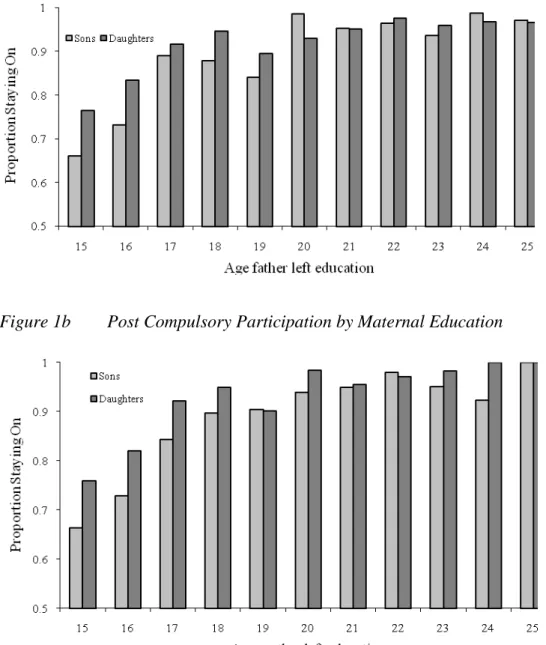
(12) systems 8. The details of the original LFS data and the impact of the selection criteria can be seen in Table 1. We select teenagers where two parents are present 9, and where the father is working and reporting his income, where both parents were born after 1933 (and so were not affected by the earlier raising of the school leaving from 14 to 15, and whose school leaving is unlikely to have been directly affected by World War II), and where both parents were born in the United Kingdom, and are currently resident in England or Wales. We make these restrictions in order to avoid including potentially endogenous factors that affect educational outcomes. Thus, our estimates need to be viewed as condition on these selections 10. We also drop any observations where there is missing data on the variables of interest and we trim the bottom 1% and top 5% of the paternal earnings distribution. Figures 1a and 1b show the participation rate in post-compulsory schooling in our final sample broken down by paternal and maternal education. The education of the children appears closely correlated with the education of their parents, particularly up to a leaving age of 18; having parents with more education than this level does not substantially affect the staying-on probability of children which is then almost 100% 11. There are some sizable gaps between the participation of girls and boys from lower educated parents but these gaps narrow with parental education. Table 2 shows some selected statistics for the sample used in our analysis. The postcompulsory schooling participation rate is 73% for boys and 83% for girls 12. There are large. 8. The data records only region of current residence, not where the parents where educated. However, this is unimportant in our IV context. Re-estimating including observations in NI and Scotland leads to a drop in precision but no change in the magnitudes of the key parameters. 9. Whilst this may create some selection bias it would be difficult to overcome this in our data. Since parental separation is probably more likely for children with large (but unobservable) propensities to leave school early, and it is also likely to be negatively correlated with parental education and income we might expect to underestimate the effect of income and education on the dependent variables. We also examined the effects of living with a stepparent but found that, while there was a negative stepparent effect, the interaction between this and education or income proved insignificant. Results are available on request.. 10. In fact, the estimated coefficients of interest were not greatly affected by these selections.. 11. Note that there are only few parents with school leaving age of 17, 19, 20 and above 23.. 12. Official statistics from the Department for Children, Schools and Families show 67% of boys and 75% of girls in the relevant cohort choosing to stay so our own staying-on figures from LFS are a little higher reflecting the selections that we have made.. 10.

(13) differences in the parental education and household income levels between those that remain in school compared to those that leave: more than one year extra parental education on average, and more than 20% higher paternal earnings. Parental income is potentially endogenous either because it is correlated with unobservable characteristics which are correlated with the child’s educational attainment, or because the parental education effect is transmitted through income. Shea (2002) estimates the impact of parental income using variation in income associated with union, industry, and job loss and finds a negligible impact on children’s human capital for most families (although parental income did seem to matter for families whose father has low education). We assume that union membership status creates an exogenous change in income, which is independent of parenting ability and the child’s educational choice. Indeed the raw data, presented in Table 1, showed that children who stay on are just as likely to have unionized fathers as children who do not stay on in education. We also exploit paternal occupation but mostly to control for differences in unionization rate by occupation. Later, the estimates that we highlight are those that rely only on paternal occupation-union interactions as exclusion restrictions, (although we find a similar pattern of results when we also use union status alone as the exclusion restriction). Lewis (1986), and much subsequent work, demonstrates that wages vary substantially with union status, controlling for observable skills. Figure 3 shows the kernel densities of the earnings of union member fathers and non-union fathers. The union/non-union earnings gap for fathers in our selected sample from the raw data is 8%. If union wage premia reflect rents rather than unobserved ability differences it seems plausible to make the (stronger) identifying assumption, used in this paper; that union status, controlling for occupation, is uncorrelated directly with the parental influence on educational outcomes of the children. Support for the view that unionization picks up differences in labour market productivity is mixed. Murphy and Topel (1990) find that individuals who switch union status experience wage changes that are small relative to the corresponding cross-section wage differences, suggesting that union premia are primarily due to differences in unobserved ability. However Freeman (1994) counters this view, arguing that union switches in panel data are largely spurious so that measurement error biases the union coefficient towards zero in the panel. In any event, we are assuming, as in Shea (2002), that unionized fathers (and their spouses) are 11.

(14) not more ‘productive’ as parents than non-union fathers with similar observable skills and we have some evidence to suggest that parenting behaviour is not very different across union status of fathers. 13 Parental education is also likely to be endogenous. Here we rely on two sources of variation. Reforms to the minimum school leaving age have frequently been used as a source of exogenous variation – either exploiting natural experiments where different areas of a country changed their rules at different times, or using a national reform as a regression discontinuity by controlling for the smooth trends in school leaving, or considering just a narrow window of birth cohorts around the reform. 14 In this paper we identify the effect of parental education on children’s education using the exogenous variation in schooling caused by the raising of the minimum school leaving age (abbreviated as RoSLA: Raising of the School Leaving Age). Individuals born before September 1957 could leave school at 15 while those born after this date had to stay for an extra year of schooling. This policy change creates a discontinuity in the years of education attained by the parents. Figures 2a and 2b illustrate this by showing mean years of schooling by birth cohort (in 4 month periods) around the reform date. That is, we take a narrow window of birth cohorts around the reform (+/- four years) to minimize the influence of any long-term trends across birth cohorts. There is a marked jump in the graph for parents born after September 1957 which coincides with the introduction of the new higher school leaving age. Note that between 30% and 40% of parents left school before the new minimum, so that the reform is biting and changes the. 13. The British Cohort Study (BCS) data, of all children born in England and Wales in a particular week in 1970, records, in considerable detail, the attitudes and behaviours of fathers towards their children. This data suggests small differences in attitudes and behaviours across union status. For example, 23% on unionised fathers disagreed with the statement that “The needs of children are more important than one’s own”, compared to 18% of the non-unionised; 60% (62%) of children with unionised (non-unionised) fathers watched TV less than 2 hours per day on a typical weekend day; 83% (88%) of unionised (non-unionised) fathers read stories more than once per week 57% (52%) of unionised (non-unionised) fathers always (as opposed to often/sometimes/never) talked to his child even when busy; 79% (79%) of unionised (non-unionised) fathers showed the child physical affection at least once per day and 36% (37%) praised the child at least once per day; 94% (95%) of unionised (non-unionised) fathers has helped young children learn numbers, etc; and 79% (80%) of unionised (nonunionised) fathers aspired for the child to continue in full-time education at age 16. The children also reported behaviour that might well reflect parenting styles. For example, 56% (54%) of the children of unionised (nonunionised) fathers made their own bed and 49% (52%) cleaned their own room. 14. See, for example, Harmon and Walker (1995) for the UK; Black, Devereux and Salvanes (2005) for Norway; and Oreopoulos, Page and Stevens, (2006) for the USA.. 12.

(15) behaviour of a substantial fraction of individuals in the affected cohorts. Individuals affected by the new school leaving age have on average completed half a year more schooling than those born just before the reform. Chevalier et al. (2004) show that the effect of this reform was almost entirely confined to the probability of leaving at 15 relative to 16 – there is little effect higher up the years of education distribution. Hence, this reform only identifies a LATE for individuals with low levels of education. Table 2 shows that the proportion of fathers who were born before the RoSLA reform is higher than for mothers, reflecting their slightly greater age, and the table also shows that early leavers typically have slightly younger parents. A second source of variation in parental schooling that we exploit derives from parental month of birth (exploited by Crawford et al. (2007)). There are several ways in which month of birth can affect the parents’ education levels: through entry timing, whole group teaching, developmental differences, and through peer effects. The academic year starts in September but the traditional admissions policy that reigned in the 1950’s and 1960’s, when most of the parents in our data were young, allowed entry at the start of the term that the child turns 5 so that there were three points of entry each year: September, January and April/May. Thus the August born would start in April/May and have two fewer terms in primary school than their classmates. A school cohort would consist of children born within a 12-month window. In the 1950’s and 60’s whole class teaching was the dominant teaching method and development differences might imply that the youngest and the oldest might fare worse than the average. Peer effects might arise because the youngest might be dominated or intimidated by the oldest. The year group moves as a single unit through the academic system so that they sit examinations at same time and would be at different development ages when facing the same examination. Moreover, most of the parents in the data would have faced a selective schooling system where children were segregated into academic or vocational schools at the age of 11 based on a single test conducted on the same day across the whole country - known as the 11+ exam. Based on the results of this test, children were educated either in vocational or academic tracks. Children in the vocational track were more likely to leave school at the minimum compulsory age, while those for the latter could go on to higher secondary school and university (see Harmon and Walker, 1997). These two different types of schools placed quite different expectations on the children and there was very little movement between 13.

(16) school types after the age of 11. Figure 4 shows, by year of birth, the average age at which the parents in our data left full-time education for those who were September born, the eldest in their class cohort, compared to those who were July born, the youngest 15. The typical difference in years of schooling between the September and July born was around ¼ of a year for these cohorts born in the 50’s and 60’s. Notice that the gap closed completely for cohorts born in the early 1960’s when the 11+ examination was abandoned in most areas. So the month of birth effect in educational achievement seems to be mostly driven by the early tracking faced by these cohorts.. 4.. Estimates Our basic model of the impact of parental background on the post-compulsory. schooling participation of their children is: (1). ′h + f ( DBc , DBm , DB f ) + ε c = PCc a ( S m , S f ) + γ Yh + Xδ. where the c, m and p subscripts refer to the child, maternal and paternal characteristics within a particular household h.. The dependent variable PCc is a dummy variable defining. participation in post compulsory education. This is estimated as a linear probability model to subsequently facilitate the use of instrumental variables 16, and is a function, a(.), of parental education levels measured in years of schooling of both the mother and father (Sm , Sf), and log parental income Yh measured by father’s real log gross weekly earnings from employment 17. DB refers to date of birth (year and month) so that f(.) controls for cohort. 15. We use July rather than August for this comparison since there is likely to be some ambiguity with Augustborn children to the extent that schools exercised discretion at the margin. 16. The marginal effects from probit estimation are very close to the linear probability model coefficient estimates and are available on request.. 17. Note that we use paternal income because the use of household income measures requires the inclusion of female earnings, which is potentially much more heavily affected by endogenous labour supply decisions. However its exclusion may also cause a bias if female labour supply is correlated with educational outcomes for children as well as with the variable of interest in the model. We share our inability to resolve this problem with the rest of the literature. If maternal labour supply is uncorrelated with paternal income and if incomes are shared within the household then our estimate of the effect of paternal income is the same as the effect of household income. This is clearly an important problem for future research.. 14.

(17) trends in paternal, maternal and child education. Three different specifications of X are used. First Xh contains characteristics common to all three members of the family (i.e. year and month of survey dummies as well as region of residence at time of survey). Second, we additionally condition for paternal occupation, so that the difference in unionization between occupations does not identify the IV model. Third, we add union status, so that the identification in the IV model only comes from the interaction terms between union status and occupation. This then captures any differences in parenting behaviour that unionized father may have. Table 3 summarizes our OLS estimates of paternal income and parental education levels, where a(.) is assumed to be linear, on the probability of post-compulsory schooling of the child 18. Specification (1) only controls for parental years of schooling and suggests positive, if modest, paternal and maternal education effects on the schooling choice of both sexes. The impact of a year of maternal education is an increase in the probability of post-16 participation of about 3.3% for boys and 2.6% for girls – about one percentage point lower than reported in Chevalier (2004). The impact of paternal education is somewhat lower and the effect on boys is larger than for girls. Specification (2) examines the impact of paternal income but excludes the parental education controls. These estimates suggest sizable and significant income elasticities with the effect somewhat larger for boys (20%) than for girls (14%). Finally specification (3) includes both education and income controls.. The direct. effects of maternal education estimated in Specification (1) are reduced very slightly in (3), but the paternal education and income effects are reduced by a factor of approximately one third compared to (1) and (2), highlighting the correlation between paternal education and income 19. 18. We control for smooth cohort trends by including a cubic function of parents and child’s months/years of birth. Region controls are also included, as well as survey year dummies. Full results are available on request. Similar estimates based on probit models are also available. While multiple observations of closely spaced children in each household are possible their incidence is small (just 10% of individuals have at least one other sibling in the dataset) and any improvement in standard errors from exploiting the clustering in the data would be marginal. 19. The estimated income effects here are closely comparable in magnitude to the results in Blanden and Gregg (2004). See their Tables 6 and 7 in particular.. 15.

(18) The second set of estimates (4, 5, 6) in Table 3 adds the paternal occupation status (7 dummies). This is potentially an endogenous variable, but since unionization rate differs by occupation, without controlling for occupation the union instrument would partially capture occupational choice which would invalidate its use. As expected, since parental occupation can be viewed as proxies for permanent income, the estimates on education are almost identical to those obtained when controlling for paternal income. Thus, in this specification, income is best interpreted as deviation from the permanent income. As such, the income effects are reduced by about 30% for boys and 50% for girls. Note, however, that when controlling for occupation, adding paternal income only marginally reduces the effect of paternal education on the educational attainment of children. Thus indicating that the correlation between paternal education and income mostly captures the permanent component of income, rather than income shocks. While we have tried to alleviate the concern that unionized fathers differ in their parenting behaviour, our final identification strategy relies only on the interactions of paternal union membership and paternal occupation as instruments for paternal income. Thus, the final set of estimates in Table 3 show the effects of parental education and paternal earnings when controlling for the effects (not interacted) of paternal union membership and paternal occupation dummies in specifications (7), (8) and (9). The effects of parental education are virtually unchanged compared to the estimates presented in (4) and (6); supporting the view that paternal union membership has no direct effect on the education decision of his children. For girls, the effect of paternal income also remains unchanged compared to specifications (5) and (6) while for boys it decreases by less than one percentage point. To summarise these results: the effect of parental education on the decision to remain in school past compulsory age appears to be quite small - around 3% for boys and 2% for girls, and larger for maternal education than parental education. The gap between the effect of maternal and paternal education increases when measures of, or proxies for, income are introduced since the maternal education effect remains largely unaffected while paternal education effect drops by almost a half. Note also that the income effects are severely reduced when a measure of permanent income is controlled for. To control for the potential endogeneity of paternal income and parental schooling we specify a set of first stage equations. We define dummy variables for RoSLA (born after the 16.

(19) critical date) and parental union membership (PUM), and its interactions with the seven occupational categories, Occ, which are incorporated into our first stage model. We also impose a linear structure on the month of birth effect 20 by including a month of birth indicator, MoB (which takes the value of one for September born through to twelve for August born). Therefore, in our preferred specification, we estimate a system of first stage equations, using a seemingly unrelated specification to allow for correlations between the respective residuals: = S m φ1 RoSLAm + φ2 MoBm + X′hφ3 + r ( DBm ) + µm. (2). = S p θ1 RoSLAp + θ 2 MoB p + X′hθ3 + s ( DB p ) + υ p. = Yp. ( PUM. p. * Occ p )′ π 1 + X′hπ 3 + ω p. where the functions r(.), and s(.) control for smooth birth cohort trends in school leaving age so that the RoSLA acts as a regression discontinuity and picks up the effects of the reform. The system of equations defined above is over-identified and we estimated a wide variety of first stages and corresponding second stage equations to examine the sensitivity of the second stage estimates to the set of exclusion restrictions used to define the instrumental variables. Our IV estimates have the property, also a feature of the OLS estimates, that the addition of income to the model containing just parental education levels makes little difference to the estimates. Thus, we refrain from presenting specifications that contain just parental income or just parental education levels 21. Table 4 shows different specifications of our three first stage equations. Each block refers to a different equation – the paternal schooling equation, the maternal schooling equation, and the paternal log earnings equation. The columns show specifications that vary according to which sets of instruments are used. The three equations are estimated simultaneously and the F-statistics of the different sets of instruments are presented in the bottom panel of the table. Comparing across the schooling equations we see that the inclusion of MoB is significant at 5% but makes little difference to the size and significance of the RoSLA effects. In general, the raising of the school leaving. 20. Greater flexibility could be sought but at the cost, of course, of potential weakness in the instruments.. 21. These results are available on request.. 17.

(20) age increased parental education by between 0.25 and 0.3 of a year, the effects being almost identical for both parents. The month of birth effect is also statistically significant and negative for both males and females. An August born child, on average, left school one sixth of a year earlier than a September born child. The two instruments identify the effects of exogenous shocks to parental education through different mechanisms - so that in models where both set of instruments are included the estimates are almost identical to the ones obtained when the instruments are included individually. So while both instruments identify a population of marginal students, these are not identical populations. The paternal earnings equation shows a significant positive union membership wage premium of 7% in columns 1, 2 and 3, which are consistent with existing UK evidence. In specifications 4, 5 and 6 the interactions of union membership and occupation show that the premium is larger for manual and less skilled occupations (the reference group being Managers and Senior Administrators). The corresponding F tests for the joint significance of all of the instruments used in each specification of the exclusion restrictions indicate whether the instruments are “weak”. The critical values of these F tests are reported in Stock and Yogo (2005) – the rule of thumb for the just identified case and one endogenous variable is approximately 10, with larger values for more exclusion restrictions. Thus our F tests vary from indicating instruments with considerable strength to being close to weak. Table 5 shows the second stage estimates 22. Specifications (a) and (b) replicate the OLS estimates from Table 3 when controlling for occupation only or for occupation and union status, respectively. The subsequent columns report the IV estimates for different specifications of the first stage. The pattern of second stage estimates of parental education effects seems remarkably stable across the IV specifications. The effect of paternal education is always imprecisely estimated when controlling for maternal education and paternal earnings regardless of which set of instruments is used and never statistically significant. Note though that the sign of the point estimates differs for sons and daughters. The effect of maternal education on daughters is between 0.187 and 0.212 depending on the instruments. 22. Table 5 reports only the OLS and IV estimates for the specifications labelled (6) and (9) in Table 3 but similar stability in the second stage results can be shown in the estimates for the equivalent of the other specifications presented in Table 3.. 18.

(21) used and is always significant at the 1% level, and significantly higher than the OLS estimate of 0.022. The magnitude of the effect of maternal schooling on the schooling of sons also increases greatly when instrumented and reaches 0.10 in all specifications but just failed to be statistically significant. Overall, the impact of maternal schooling on the schooling decisions of her children, and especially daughters, appear to be quite large. The effect of paternal earnings varies with the instruments used. When Paternal Union Membership alone is used as an instrument, the effect is roughly 0.26 for sons and 0.29 for daughters. If occupation, union membership and interactions of occupation and union membership are used, the effect of paternal income becomes larger for sons (0.32) but decreases (to 0.13) for daughters. However, in our preferred specification, when only the interactions of union and occupation are used as instrument and both union and occupations are controlled for, the effect of paternal income becomes much smaller especially for daughters. Even if the point estimates are still large for sons, they are statistically insignificant at even the 10% level. Thus, paternal earnings, that we take as a measure of short term variation in the household income as we are controlling for occupation, have little impact on the schooling decisions of children. 5.. Conclusion This paper has addressed the intergenerational transmission of education and. investigated the extent to which early school leaving (at age 16) may be due to variations in permanent income and parental education levels. Least squares revealed conventional results - stronger effects of maternal than paternal education, and stronger effects on sons than daughters. We also found that the education effects remained significant even when household income was included. Income remains significant even when some measures of permanent income are included which indicates that some children could be financially constrained in their decision to attend post-compulsory education. When controlling for paternal income, the IV results reinforce the role of maternal education, especially for daughters, where the estimates increase almost ten fold. One year of maternal education, for mothers affected by our instruments, increases the probability of her daughter staying on by 20 percentage points. The effects on sons are only half of this and just on the border of statistical significance. In contrast, paternal education has no statistical effect on the probability of remaining in educations for either son or daughter. 19.

(22) Accounting for the endogeneity of paternal income also increases the elasticity of income on schooling decisions, however depending on the set of instruments the effects is imprecisely estimated, and in our preferred specification becomes insignificant, even if a large point estimate is still found for sons. The income effects are in general larger for boys than for girls, this is also the case for the UK’s Education Maintenance Allowance (EMA). The results imply that policy options that are explicitly aimed at relieving credit constraints at the minimum school leaving age such as EMA (see Dearden et al., 2010 ) may not be so effective in promoting higher levels of education (a finding that is consistent with recent UK evidence that used linked administrative data for a cohort from age 11 to age 19 – see Chowdry et al, 2010). A policy of increasing permanent income, like increasing parental education (or say through Child Benefit) would on the other hand have some positive effects, especially for daughters. The recently proposed increase of the school leaving age to 18 would also benefit future generations through direct intergenerational transmission of educational choice.. 20.

(23) References Acemoglu, Daron. and Pischke, Jorn-Steffan (2001), “Changes in the Wage Structure, Family Income and Children’s Education”, European Economic Review, 45, 890–904. Almond, Douglas and Currie, Janet. (2009), “Human Capital Development before Age Five”, mimeo. Antonivics, Karen and Goldberger, Arthur (2005),. “Does Increasing Women’s Schooling Raise the Schooling of the Next Generation? Comment”, American Economic Review, 95, 1738-1744 Behrman, Jere. (1997), “Mother’s Schooling and Child Education: A Survey.” University of Pennsylvania Department of Economics, DP 025. Behrman Jere and Rosenzweig, Mark (2002), “Does Increasing Women’s Schooling Raise the Schooling of the Next Generation.” American Economic Review, 92, 323-334 Behrman Jere, Rosenzweig, Mark and Zhang, J (2005),. “Does Increasing Women’s Schooling Raise the Schooling of the Next Generation. Reply”, American Economic Review, 95, 1745-1751. Bjorklund, Anders, Lindahl, Mikael and Plug, Erik (2006), “The Origins of Intergenerational Associations: Lessons from Swedish Adoption Data”, Quarterly Journal of Economics, 121, 999-1028. Bjorklund, Anders and Salvanes, Kjell (2010), “Education and Family Background”, IZA Discussion Paper 5002. Black, Sandra E., Devereux, Paul J. (2010), “Recent Developments in Intergenerational Mobility”, National Bureau of Economic Research, WP15889. Black, Sandra E., Devereux, Paul J. and Salvanes, K.G. (2005), “Why the Apple Doesn't Fall Far: Understanding Intergenerational Transmission of Human Capital”, American Economic Review, 95, 437-449. Blanden, Jo and Gregg, Paul (2004),. “Family Income and Educational Attainment: A Review of Approaches and Evidence for Britain”, Oxford Review of Economic Policy, 20, 245-263 Cameron Stephen and Heckman, James J. (19898), “Life Cycle Schooling and Dynamic Selection Bias: Models and Evidence for Five Cohorts of American Males”, Journal of Political Economy, 106, 262-333 Carneiro Pedro and Heckman, James J. (2004), “Human Capital Policy.” In James J. Heckman and Alan B. Krueger, eds., Inequality in America. Cambridge: MIT Press. Carneiro, Pedro, Costas Meghir and Matthias Parey (2007), “Maternal Education, Home Environments and the Development of Children and Adolescents”, IZA Discussion Paper No. 3072. Chevalier, Arnaud (2004), “Parental Education and Child's Education: A Natural Experiment”, IZA Discussion Paper No. 1153,. Chevalier Arnaud, Harmon, Colm, Walker, Ian and Zhu, Yu (2004) “Does Education Raise Productivity or Just Reflect It?”, Economic Journal, 114, F499-F517. 21.

(24) Chevalier Arnaud and Lanot, Gauthier (2002), “The Relative Effect of Family Characteristics and Financial Situation on Educational Achievement.” Education Economics, 10, 165-182. Chowdry, Haroon, Crawford, Claire, Dearden, Lorraine, Goodman, Alissa; and Vignoles, Anna (2010), “Widening Participation in Higher Education: Analysis Using Linked Administrative Data.” Institute for Fiscal Studies Working Paper W10/04. Currie, Janet and Moretti, Enrico (2003), “Mother’s Education and the Intergenerational Transmission of Human Capital: Evidence from College Openings and Longitudinal Data”, Quarterly Journal of Economics, 118, 1495-1532 Dearden, Lorraine (2004), “Credit Constraints and Returns to the Marginal Learner”, Institute for Fiscal Studies, mimeo,. Dearden, Lorraine, Emmerson, Carl, Frayne, Christina and Meghir, Costas. (2009) “Conditional Cash Transfers and School Dropout Rates.” Journal of Human Resources, 44, Ermisch, John and Francesconi, Marco (2001), The effect of parents' employment on outcomes for children, Joseph Rowntree Foundation. Feldman Marcus W., Otto, Sarah P. and Christiansen, Freddy B. (2000), “Genes, culture and inequality” in Kenneth Arrow, Samuel Bowles and Steven Durlauf, eds., Meritocracy and Economic Inequality. Princeton: Princeton University Press. Freeman, Richard B. (1994), “H.G. Lewis and the Study of Union Wage Effects”, Journal of Labor Economics, 12, 143-149. Galindo-Rueda, Fernando (2003), “The Intergenerational Effect of Parental Schooling: Evidence from the British 1947 School Leaving Age Reform.” Centre for Economic Performance, London School of Economics, mimeo. Gregg, Paul, Harkness, Susan and Machin, Stephen (1999), “Poor Kids: Child Poverty in Britain, 1966-1996.” Fiscal Studies, 20, 163-187. Harmon Colm and Walker, Ian (1995), “Estimates of the Economic Return to Schooling in the United Kingdom”, American Economic Review, 85, 1278-1286. Heckman, James J. and Masterov, Dimitri V. (2005), “Skills Policies for Scotland”. In Diane Coyle, Wendy Alexander and Brian Ashcroft (Eds). New Wealth for Old Nations: Scotland’s Economic Prospects, Princeton University Press. Holmlund, Helena, Mikael Lindahl, and Erik Plug (2008) “The Causal Effect of Parent's Schooling on Children's Schooling: A Comparison of Estimation Methods”, IZA Discussion Paper No. 3630. Imbens, Guido and Angrist, Joshua (1994), “Identification and Estimation of Local Average Treatment Effects”, Econometrica, 62, 467-475 Jenkins, Stephen P. and Schluter, Christian (2002), “The Effect of Family Income During Childhood on Later-Life Attainment: Evidence from Germany”, DIW Discussion Paper 317. Krueger, Alan B. (2004), “Inequality, Too Much of a Good Thing.” In James J. Heckman and Alan B. Krueger, eds., Inequality in America, Cambridge: MIT Press 22.

(25) Lewis, H. Gregg (1986), . Union Relative Wage Effects: A Survey,Chicago: University of Chicago Press. Loken, Katrine, V. (2010), “Family income and children’s education: Using the Norwegian oil boom as a natural experiment”, Labour Economics, 17, 118-129. Maughan, Barbara, Collishaw, Stephan M. and Pickles, Andrew, (1998), “School Achievement and Adult Qualifications Among Adoptees: a Longitudinal Study.” Journal of Child Psychology and Psychiatry, 39, 669-686. Maurin, Eric and Sandra McNally. (2008), “Vive la Révolution! Long Term Returns of 1968 to the Angry Students”, Journal of Labour Economics 26, 1-33. Meyer, S. (1997), What Money Can’t Buy: Family Income and Children’s Life Chances, Cambridge: Harvard University Press. Mulligan Casey (1999), “Galton Versus the Human Capital Approach to Inheritance.” Journal of Political Economy, 107, 184-224 Murphy, Kevin and Topel, Robert (1990), “Efficiency Wages Reconsidered: Theory and Evidence.” In Weiss, Y., Fishelson, G., eds., Advances in the Theory and Measurement of Unemployment, Macmillan: London, 204-242. Oreopoulous, Philip, Page, M. and Stevens, A. (2006), “The Intergenerational Effects of Compulsory Schooling.” Journal of Labour Economics, 24, 729-760.. Page, Marianne E. (2009), “Fathers’ education and children’s human capital: Evidence from the world war II G.I. Bill”, mimeo. Plug, Erik. (2004) “Estimating the effect of mother’s schooling and children’s schooling using a sample of adoptees”. American Economic Review, 94, 358-368. Sacerdote, Bruce (2007), “What Happens When We Randomly Assign Children to Families”, Quarterly Journal of Economics, 122, 119-157 Sanbonmatsu, Lisa, Jeffrey, J.R., Kling, G.R., Duncan, G.J. and Brooks-Gunn, J. (2006), “Neighborhoods and Academic Achievement: Results from the Moving to Opportunity Experiment.” Journal of Human Resources, 41, 649-691. Shea, John (2002), “Does Parents' Money Matter?”, Journal of Public Economics, 77, 155184 Smith, Richard and Blundell, Richard (1986), “An Exogeneity Test for a Simultaneous Equation Tobit Model with an Application to Labor Supply.” Econometrica, 54, 679686. Solon, Gary (1999), “Intergenerational Mobility in the Labor Market”, in Orley Ashenfelter and David Card, eds., Handbook of Labor Economics – Vol. 3A, Amsterdam: North Holland. Stock, J. H., and M. Yogo. (2005), “Testing for Weak Instruments in Linear IV Regression”, in D.W. Andrews and J. H. Stock (eds), Identification and Inference for Econometric Models: Essays in Honor of Thomas Rothenberg, Cambridge University Press. UK Department for Education and Skills (2002), “Education Maintenance Allowance: The First Two Years, A Quantitative Evaluation”, Research Report 352, London: DfES. 23.

(26) Figure 1a. Post Compulsory Participation by Paternal Education. Figure 1b. Post Compulsory Participation by Maternal Education. 24.

(27) Figure 2a Distribution of paternal school leaving age by third of year of birth. Figure 2b Distribution of maternal school leaving age by third of year of birth. 25.

(28) Figure 3: Distribution of father’s weekly earnings by union status union. non-union. .002. .0015. .001. .0005. 0 0. 500. 1000 dad:rwkpay. 1500. Figure 4:. Average School Leaving Age by Year of Birth: England Only. Table 1:. Sample selection 26. 2000.

(29) Living Away from parents. Living with one parent. Living with both parents. Final sample. % aged 16. 1.99. 10.06. 10.89. 10.29. % aged 17. 33.82. 47.45. 48.94. 46.87. % aged 18. 64.19. 42.49. 40.17. 42.84. % Staying on at 16. 26.99. 71.06. 75.85. 77.53. % Attaining 5+ GCSE A*-C. 39.68. 67.16. 76.54. 78.07. 2,836. 9,035. 31,103. 8,367. Age distribution:. Observations:. Note: The following are dropped from the penultimate column to form the final sample: families where father is not working or self employed or has no or missing reported earnings (approximately nine thousand); families where one or both parents are immigrants (approximately five thousand); very old or very young parents (approximately four hundred); families residing in Scotland and in heavily oversampled Northern Ireland (approximately five thousand); observations missing other information (approximately fourteen hundred); and the bottom 1% and top 5% of the father’s earnings distribution (approximately seven hundred).. 27.

(30) Table 2. Descriptive Statistics: LFS 1992-2006 – Estimation Sample. Paternal Log Earnings. Paternal School Leaving Age. Maternal School Leaving Age. Maternal Age. Father affected by RoSLA. Mother Affected by RoSLA. Paternal Union Membershi p. Paternal Age. Age of Respondent. 6.04. 15.93. 15.93. 45.41. 43.52. 0.31. 0.23. 0.41. 17.32. (0.43). (1.48). (1.25). (5.51). (4.84). (0.46). (0.42). (0.49). (0.65). 6.31. 17.28. 17.17. 47.09. 45.03. 0.26. 0.18. 0.43. 17.32. (0.50). (2.61). (2.23). (5.08). (4.49). (0.44). (0.38). (0.50). (0.65). 6.27. 17.04. 16.95. 46.80. 44.77. 0.27. 0.19. 0.43. 17.32. (0.50). (2.50). (2.15). (5.19). (4.59). (0.44). (0.39). (0.50). (0.65). 6.07. 15.97. 16.00. 45.36. 43.31. 0.34. 0.23. 0.40. 17.35. (0.45). (1.45). (1.25). (5.04). (4.62). (0.47). (0.42). (0.49). (0.64). 6.33. 17.49. 17.33. 47.05. 45.10. 0.24. 0.16. 0.43. 17.32. (0.50). (2.73). (2.32). (4.97). (4.52). (0.43). (0.36). (0.49). (0.66). 6.26. 17.08. 16.97. 46.60. 44.62. 0.27. 0.18. 0.42. 17.33. (0.50). (2.55). (2.17). (5.05). (4.62). (0.44). (0.38). (0.49). (0.65). Girls: N= 4024 Did not stay in full time education (17%): Did stay in full time education (83%): All. Boys: N= 4343 Did not stay in full time education (27%) Did stay in full time education (73%) All Note: Selected means, standard deviation in brackets. 28.

(31) Table 3. Effects of Parental Education and Income on the Probability of Post-Compulsory Schooling of Children Specification:. 1. 2. 3. 4. 0.033. 0.031. 0.029. 0.004. 0.004. 0.004. 0.025. 0.017. 0.003. 0.003. 5. 6. 7. 8. 9. 0.029. 0.029. 0.028. 0.004. 0.004. 0.004. 0.014. 0.012. 0.014. 0.012. 0.003. 0.003. 0.003. 0.003. BOYS: N=4343 Maternal School Leaving Age Paternal School Leaving Age Paternal Log Earnings. 0.195. 0.123. 0.113. 0.085. 0.014. 0.015. 0.016. 0.016. 0.105. 0.078. 0.017. 0.017. GIRLS: N= 4024 Maternal School Leaving Age Paternal School Leaving Age. 0.026. 0.024. 0.022. 0.003. 0.003. 0.003. 0.016. 0.010. 0.008. 0.003. 0.003. 0.003. Paternal Log Earnings Controls for paternal union membership. no. 0.14 0.013. 0.093 0.014. no. no. no. 0.022 0.003. 0.022 0.003. 0.007 0.003. 0.003. 0.008. 0.007. 0.003. 0.068 0.015. 0.049 0.015. no. no. yes. no no no yes yes yes yes Control for paternal occupation Note: LFS 1992-2006. Standard errors in italics. Specifications 1, 2 and 3 include year of survey dummies, regional dummies, dummies of child’s date of birth, dummies in the date of birth of both parents in five year intervals.. 29. 0.022. 0.003 0.065 0.015. 0.047 0.016. yes. Yes yes. yes.

(32) Table 4: First Stage Regressions. Maternal Paternal schooling Schooling. N=8,367 Paternal RoSLA. 1 0.270 0.098. Paternal MoB Maternal RoSLA. -0.015 0.006 0.278 0.08. Maternal MoB Paternal Union Membership (PUM). 2. 0.072 0.009. -0.016 0.006 0.072 0.009. 3 0.250 0.099 -0.014 0.006 0.255 0.08 -0.014 0.006 0.072 0.009. PUM *Professional. Paternal earnings. PUM*Lower Professional PUM*Admin & Secretarial PUM*Skilled Trade PUM*Personal Services PUM*Machine Operatives. F stats, p values. PUM*Elementary Occupations 7.44, 0 6.57, 0 5.13, 0.01 7.01, 0. 4 0.278 0.102. 5. -0.015 0.007 0.284 0.08. 0.049 0.018 0.009 0.027 0.005 0.032 0.102 0.043 0.106 0.027 0.304 0.042 0.117 0.028 0.208 0.039 9.00, 0. -0.016 0.006 0.049 0.018 0.009 0.027 0.004 0.032 0.102 0.043 0.106 0.027 0.304 0.042 0.117 0.028 0.208 0.039. RoSLA MoB RoSLA and MoB Occ. 8.88, 0. PUM PUM, Occ., PUM*Occ. PUM*Occ. PUM, PUM*Occ. 59.82, 0 59.82, 0 59.82, 0 7.28, 0.01 7.28, 0.01 187.39,0 187.39,0 13.34, 0 13.34, 0 37.24, 0 37.24, 0. 6.21, 0 290.14, 0 290.14. Parental Education IVs, PUM 25.8,0 24.25, 0 17.54, 0 Parental Education IVs, PUM, Occ, PUM*Occ Parental Education IVs, PUM*Occ Parental Education IVs, PUM, PUM*Occ. 6 0.258 0.102 -0.013 0.007 0.261 0.081 -0.014 0.006 0.049 0.018 0.009 0.027 0.004 0.032 0.102 0.043 0.106 0.027 0.304 0.042 0.117 0.028 0.208 0.039 7.58, 0 4.79, 0.01 6.90, 0 290.14, 0 7.28, 0.01 187.44, 0 13.34, 0 37.24, 0. 8.43, 0 6.56, 0 6.98, 0 166.47,0 166.1, 0 149.46, 0 12.38, 0 11.77, 0 31.58 31.021. 11.00, 0 27.11,0. Note: Standard errors in italic. The models also include year of survey dummies, regional dummies, dummies of child’s date of birth, dummies in the date of birth of both parents in five year intervals and dummies for paternal occupation. RoSLA is a dummy for the Raising of School Leaving Age, MoB stands for Month of birth (a linear function on month with September = 1 to August = 12); PUM is Paternal Union Membership Status; and Occ is paternal occupation (7 categories). 30.

(33) Table 5. Instrumental Variable Estimates: LFS 1992-2006. Specification:. a. Instruments. b. 1. 2. 3. 4. 5. 6. -. RoSLA. RoSLA. RoSLA. RoSLA. RoSLA. RoSLA. Mob PUM. MoB. PUM. PUM. MoB. PUM. PUM*Occ PUM*Occ PUM*Occ PUM*Occ PUM. PUM. PUM. Occ. Occ. Occ. 0.102. 0.102. 0.102. 0.102. 0.058. 0.059. 0.058. 0.059. 0.058. 0.026. 0.021. 0.028. 0.023. 0.037. 0.031. 0.003. 0.046. 0.044. 0.045. 0.043. 0.046. 0.044. 0.085. 0.078. 0.258. 0.261. 0.317. 0.319. 0.214. 0.219. 0.016. 0.017. 0.092. 0.092. 0.078. 0.078. 0.140. 0.140. 0.022. 0.022. 0.214. 0.189. 0.212. 0.188. 0.211. 0.187. 0.003. 0.003. 0.055. 0.053. 0.055. 0.054. 0.055. 0.054. 0.007. 0.007. -0.091. -0.061. -0.067. -0.040. -0.061. 0.04. 0.003. 0.003. 0.044. 0.041. 0.043. 0.040. 0.043. 0.04. 0.049. 0.047. 0.286. 0.274. 0.136. 0.129. 0.063. 0.052. Second stage controls Occ. Occ. Occ. Occ. Occ. 0.029. 0.028. 0.004. 0.102. 0.101. 0.004. 0.059. 0.012. 0.012. 0.003. BOYS: N=4343 Maternal School Leaving Age Paternal School Leaving Age Paternal Log Earnings GIRLS: N=4024 Maternal School Leaving Age Paternal School Leaving Age Paternal Log Earnings. 0.015 0.016 0.08 0.08 0.071 0.07 0.092 0.091 Notes: Standard errors in italics. All second stage specifications include year of survey dummies, regional dummies, dummies of child’s date of birth, and dummies in the date of birth of both parents in five year intervals. RoSLA is a dummy for the Raising of School Leaving Age, Mob stands for Month of birth (linear), PUM for Paternal Union Status, and Occ for Paternal occupation (7 categories). 31.

(34)

No results found