Discussion Paper: 2011/02
Identification and inference in a simultaneous
equation under alternative information sets and
sampling schemes
Jan F. Kiviet
www.feb.uva.nl/ke/UvA-Econometrics
A
msterdam
S
chool of
E
conomics
Department of Quantitative Economics Valckenierstraat 65-67
1018 XE AMSTERDAM The Netherlands
Identi…cation and inference in a simultaneous equation
under alternative information sets and sampling schemes
Jan F. Kiviet
y9 August 2012
JEL-classi…cation: C12, C13, C15, C26, J31
Keywords:
partial identi…cation, weak instruments, (un)restrained repeated
sampling, (un)conditional (limiting) distributions, credible robust inference
Abstract
In simple static linear simultaneous equation models the empirical distributions of IV and OLS are examined under alternative sampling schemes and compared with their …rst-order asymptotic approximations. We demonstrate that the limiting distribution of consistent IV is not a¤ected by conditioning on exogenous regressors, whereas that of inconsistent OLS is. The OLS asymptotic and simulated actual variances are shown to diminish by extending the set of exogenous variables kept …xed in sampling, whereas such an extension disrupts the distribution of IV and deteriorates the accuracy of its standard asymptotic approximation, not only when instruments are weak. Against this background the consequences for the identi…cation of parameters of interest are examined for a set-ting in which (in practice often incredible) assumptions regarding the zero correlation between instruments and disturbances are replaced by (generally more credible) inter-val assumptions on the correlation between endogenous regressor and disturbance. This yields OLS-based modi…ed con…dence intervals, which are usually conservative. Often they compare favorably with IV-based intervals and accentuate their frailty.
1. Introduction
We approach the fundamental problems of simultaneity and identi…cation in econometric linear structural relationships in a non-traditional way. First, we illustrate the e¤ects of the chosen sampling regime on the limiting and empirical …nite sample distributions of both OLS (ordinary least-squares) and IV (instrumental variables) estimators. We distinguish sampling schemes
Division of Economics, School of Humanities and Social Sciences, Nanyang Technological University, 14 Nanyang Drive, Singapore 637332 ([email protected]) and Department of Quantitative Economics, Amster-dam School of Economics, University of AmsterAmster-dam, Valckenierstraat 65, 1018 XE AmsterAmster-dam, The Nether-lands ([email protected]).
yFor the many constructive remarks regarding earlier stages of this research I want to thank editor Elie
Tamer, two anonymous referees, and seminar participants at the universities of Amsterdam, Montréal, Yale (New Haven), Brown (Providence), Harvard (Cambridge), Carleton (Ottawa), New York, Penn State (Univer-sity Park), Rutgers (New Brunswick) and Columbia (New York), and those giving feedback at presentations at ESWC (Shanghai, August 2010), EC2 (Toulouse, December 2010), CESifo (Munich, February 2011) and the SER Conference (Singapore, August 2011).
in which exogenous variables are either random or kept …xed. We …nd that, apart from its shifted location due to its inconsistency, the OLS distribution is rather well-behaved, though mildly dependent on the chosen sampling regime, both in small and in large samples. On the other hand, and not predicted by standard asymptotic theory, the sampling regime is found to have a much more profound e¤ect on the actual IV distribution. Especially for …xed and not very strong instruments, IV is in fact often much less informative on the true parameter value than OLS is. Next, following ideas from the recent partial identi…cation literature1, we
then dare to replace the standard point-identifying but in practice often incredible assumption on the zero correlation between (possibly weak) instruments and the disturbance term by an alternative identifying information set. We demonstrate that identi…cation can also be obtained by abstaining from instruments altogether, by adopting instead a restricted range of possible values for the correlation between endogenous regressor and disturbance. Choosing this range wide leads to a gain in credibility and robustness, but at the expense of precision. In principle this approach and the standard approach are equally (un)feasible, because both are based on statistically untestable presuppositions.
Achieving identi…cation through replacing orthogonality conditions by simultaneity as-sumptions yields con…dence intervals which are purely based on standard OLS statistics. These have just to be transformed by a very simple formula, which involves: both the endpoints of the assumed interval for the simultaneity correlation coe¢ cient, the sample size, and a stan-dard Gaussian or Student critical value. The simplicity of the procedure is partly based on the following truly remarkable result regarding the asymptotic variance of OLS under simultaneity. This asymptotic variance is smaller (in a matrix sense) than the standard expression that holds under classic assumptions. Under the adopted partial identi…cation assumption, however, the OLS estimator is corrected for its inconsistency by a term based on standard OLS results and on the assumed simultaneity coe¢ cient. Because this correction is random, it yields an increment to the asymptotic variance of inconsistent OLS. Under normality and adopting the conservative unconditional sampling scheme, this modi…ed OLS estimator is found to have an asymptotic variance identical again to the classic well-known simple expression.
The limiting distribution of inconsistent OLS has been examined before (Goldberger, 1964; Rothenberg, 1972; Schneeweiss, 1980; Kiviet and Niemczyk, 2012), but the e¤ects of (not) conditioning on exogenous variables have not yet been studied in a systematic way. Here we provide the framework to do so, but in order to keep the derivations transparent we re-strict ourselves to results for single regressor models. Unconditional IV estimation received little attention in the literature, possibly because in the standard case conditioning has no consequences asymptotically. Early studies on the small sample distribution of method of moments estimators in static simultaneous equations (Sawa, 1969; Mariano, 1973; Phillips, 1983), all focussed on the case of …xed instruments. The more recent literature on the e¤ects of weak instruments took o¤ in Nelson and Startz (1990a,b). They adopted even more se-vere conditioning restrictions, leading to extreme correlation between structural and reduced form disturbances, as noted by Maddala and Jeong (1992). Next a literature developed in which only observed instruments are kept …xed again (Woglom, 2001; Hillier, 2006; Forchini, 2006; Phillips 2006, 2009; Andrews and Stock, 2007a), although in some studies that analyze weak/many instrument asymptotic frameworks attention is also paid to random instruments (Staiger and Stock, 1997; Andrews and Stock, 2007b). Here we will systematically examine and compare the consequences of three stages of conditioning on simple IV and OLS estimation,
1See Manski (2003, 2007) and for a recent review see Tamer (2010). Phillips (1989) and others have used
both asymptotically and experimentally.
Concerns about identi…cation and alternative approaches to achieve identi…cation in simul-taneous equations models can be found in many econometric studies. Since the validity of instruments can only be tested statistically under the maintained hypothesis of a su¢ cient number of valid instruments to achieve just identi…cation, other arguments than empirical-statistical ones are required to validate the initial set of identifying conditions. Recently, such argumentation - based either on common sense reasoning or economic theory - has often been used convincingly by designing empirical research in the format of natural or quasi-experiments, see (references in and the discussions on) Angrist and Pischke (2010). Doubts about instrument validity can also be alleviated through replacing exclusion restrictions by point or interval as-sumptions (Kraay, 2012; Conleyet al., 2012), or by allowing instruments to be correlated with structural disturbances, but less so than the endogenous regressor (Nevo and Rosen, 2012), or in the context of treatment response analysis by making so-called monotone instrumental variable assumptions (Manski and Pepper, 2000, 2009). All these approaches enable to obtain inference in the form of con…dence intervals which are asymptotically valid under the relaxed alternative assumptions that they require. The inference that we will produce here is unique in the sense that no assumptions on external instruments have to be made at all; the identifying information exploited relates directly to the degree of simultaneity. Whether in a particu-lar situation this approach is preferable does not simply depend on objective characteristics of the case under study, because the actual credibility of alternative assumptions to achieve identi…cation is inherently subjective and cannot be measured objectively on a simple ordinal scale.
Correlation between regressors and disturbances also occurs in models allowing for measure-ment errors, but then the degree of simultaneity is directly related to the parameters of primary interest and the assumptions made regarding the distribution of the errors in the variables. Studies in that context with similar aims as the present study are Kapteyn and Wansbeek (1984), Erickson (1993) and Hu (2006), but their results cannot directly be converted to the classic simultaneous equations model.
The structure of this paper is as follows. In Section 2 we sketch the various settings that we will examine regarding DGP (data generating process), alternative adopted information sets and di¤erent sampling schemes. In Section 3 the limiting and simulated …nite sample distributions of IV and OLS are examined under these various settings. Section 4 demonstrates how inference can be based just on OLS results and an assumed interval for the simultaneity coe¢ cient. It also compares its accuracy with best-practice IV-based methods in a simulation study, and illustrates the empirical consequences for the well-known Angrist and Krueger (1991) data. Finally Section 6 concludes.
2. DGP, information sets, sampling schemes
The DGP involves just two jointly dependent data series and one external instrument, from which any further exogenous explanatory variables have been partialled out. Generalizations with more than one endogenous regressor, overidenti…cation and explicit exogenous regressors are left for future work. Despite its simplicity, this DGP already embodies various salient features met in practice when analyzing actual relationships, especially when based on a cross-section sample. After its speci…cation, we discuss the various settings under which the re-lationship might be analyzed in practice. These settings di¤er regarding two aspects, being characteristics of the adopted information set and of the assumed relevant sampling scheme.
The latter relates to conditioning (or not) on random exogenous variables and the former to the available information in the form of observed data and of adopted parametric restrictions.
2.1. The DGP
Instead of specifying the analyzed model and the underlying DGP top-down, as is usually done in econometrics, we introduce these here bottom-up, following precisely the generating scheme as used in the simulation experiments that will be exploited later. The basic building block of the DGP consists of three series (for i= 1; :::; n) of IID zero mean random variables
"i IID(0; 2"); vi IID(0;
2
v ) and zi IID(0; 2z); (2.1)
which are also mutually independent. To avoid particular pathological cases we assume 2
" >0
and 2
z > 0; but allow 2v 0: The "i will establish the disturbance term in the single
simultaneous equation of interest with just one regressorxi:The reduced form equation for this
regressor xi has reduced form disturbance vi; which consists of two independent components,
since
vi =vi + "i: (2.2)
Variable zi is to be used as instrument. The reduced form equation forxi is
xi = zi+vi; (2.3)
and the simultaneous equation under study is
yi = xi+"i: (2.4)
So, in total we have 6 parameters, namely 2
"; 2v ; 2z; ; and ;where the latter is the
para-meter of primary interest. However, some of these parapara-meters can be …xed arbitrarily, without loss of generality. We may take = 0;hence acting as if we had …rst subtracted xi form both
sides of (2.4). Also, we may take z = 1 and next interpret as the original z: Moreover,
scaling equation (2.4) by taking "= 1 has no principle consequences either. So, we …nd that
this DGP has in fact only three fundamental parameters, namely ; and 2v : Nevertheless,
it represents the essentials of a general linear just identi…ed (provided 6= 0) simultaneous equation with one endogenous regressor, where any further exogenous explanatory variables, including the constant, have been netted out.
We shall consider a simple nonlinear reparametrization, because this yields three di¤erent basic parameters which are easier to interpret. Not yet imposing the normalizations ( z = 1 =
") we …nd
Cov(xi; "i) = x" x " = 2" and Cov(xi; zi) = xz x z = 2z: (2.5)
The correlations x" and xz parametrize simultaneity and instrument strength respectively.
Because the instrument obeys the moment restrictionsE(zi"i) = 0(thus z" = 0) andE(zivi) =
0; we also …nd V ar(xi) = 2x = 2 2z+ 2v; (2.6) with V ar(vi) = 2v = 2v + 2 2 "; (2.7) thus V ar(vi) = 2v = x2(1 2x" 2xz); (2.8)
and from 2 v 0 it follows that 2 x"+ 2 xz 1: (2.9)
So, only combinations of x" and xz values in or on a circle with radius unity are admissible. Such a restriction is plausible, because, given thatzi is uncorrelated with"i;regressorxi cannot
be strongly correlated with both "i and zi at the same time.
The above derivations yield a more insightful three-dimensional parameterization for this DGP. This is based on simply choosing values for x >0; x" and xz; respecting (2.9). Next
the data can be generated according to the equations (2.1) through (2.4), where
= xz x= z and = x" x= "; (2.10)
with 2
v as in (2.8), and taking " = z = 1 and = 0:
Another basic model characteristic often mentioned in this context is the population con-centration parameter (P CP), given by
P CP nV ar( zi) V ar(vi) =n 2 2 z 2 v + 2 2 " =n 2 xz 1 2 xz : (2.11)
We control this simply by setting values for xz and n: These two, together with x" and x;
and the further distributional characteristics (third and higher moments) of the IID variables
"i; vi andzi;will determine the actual properties of any inference technique for in this model.
2.2. Alternative information sets
Despite its simplicity the data generation scheme above for the relationship (2.4) is to be used to represent the essentials of particular practically relevant modelling situations, in which the ultimate goal is to produce inferences regarding : These inferences should preferably be: in-terpretable (identi…ed), accurate (supplemented by relatively precise probability statements), credible (based on nonsuspect assumptions), robust (valid under a relatively wide set of as-sumptions) and relatively e¢ cient (small absolute or mean squared errors). Although they have to be obtained from a …nite actual sample they will generally be based on asymptotic approximations to the distributions of estimators and test statistics. To derive these we have to make assumptions. Regarding these we will compare a few alternative sets. These information sets are characterized by whether particular variables are supposed to be available or not and by particular adopted parametric restrictions.
We will assume throughout that the variablesyi andxihave been observed and are available
to the practitioner, but not the disturbances"i; vi andvi:We will distinguish settings in which
zi is available too, and is used as an instrument, but also the situation in which it is not used.
Instrument zi may not be used because: (i) it is not available, (ii) because the researcher
(possibly erroneously) assumes that x" = 0, or (iii) the researcher is not willing to make the assumption z" = 0; because it seems incredible. In these cases OLS may be used, althoughxi
establishes an invalid instrument when x"6= 0:
So, regarding parametric restrictions, we will consider the situation where one is either willing to make the assumption z" = 0; or not. In addition, we will consider the situation where one is prepared to make an assumption regarding x" of the from x"2 Rx" Lx"; Ux" ;
or not. Below we will show that under x" 2 Rx" coe¢ cient can be identi…ed and analyzed
accurately by a modi…ed version of OLS, which does not require any instruments. In a way this brings IV and OLS on a comparable base: IV requires the statistically unveri…able (and
therefore often incredible) assumption z" = 0; whereas the modi…ed OLS technique requires the generally unveri…able assumption x" 2 Lx"; Ux" ;which can be made more credible (at the
expense of precision) by choosing a wider interval. A similar though fundamentally di¤erent approach is followed by Nevo and Rosen (2012) who adopt an interval for z":
2.3. Alternative sampling schemes
When running the experiments required to obtain the …nite sample distribution of estimators of we have the choice to draw new independent series for the three random variables of (2.1) every replication, or to keep the series for eitherzi orvi;or for both, …xed. By keeping none of
the series which are exogenous regarding "i …xed, we will examine unconditional distributions.
This seems especially relevant in the context of a cross-section analysis where the random sam-ple ofn observations is obtained from a much larger population. Each Monte Carlo experiment should then mimic that a new independently drawn sample does not only yield di¤erent values for the disturbances, but also for the instruments, and for the component of the reduced form disturbances which is not associated with "i:
However, in the other extreme, when the sample covers the whole population and hence establishes a census, the situation is di¤erent. Then the "i; which represent the e¤ects of
variables not explicitly taken into account into the model, should still be redrawn every exper-iment, but there are good reasons to condition on one speci…c realization of the zi; in order
to keep close to the population under study. And since the vi represent all the further typical determinants of xi;in addition to zi;which are not associated with"i, one can argue that one
would even keep closer to the characteristics of the actual population by keeping vi …xed as well, despite the fact that in practice vi is not observed. That would lead then to conditioning on latent variable xi; where
xi = zi+vi: (2.12)
When the data establish time-series there is no clear-cut population and there are good reasons to condition inference on the actual realized values of all the exogenous determinants of the endogenous variables. Note that xi = xi + "i with E(xi"i) = 0; so xi is exogenous, and –
if available –would establish the strongest possible instrument for xi, since E(xixi) = 2x =
2
x(1 2x") and hence, due to (2.9),
2 x x= 4 x(1 2x")2 4 x(1 2x") = 1 2x" 2xz: (2.13)
In the present context, as will be shown in the next section, the limiting distribution of consistent estimators is invariant with respect to whether or not one conditions on exogenous variables. Therefore, inference based on asymptotic arguments is not directly a¤ected, which explains why the issue of sampling schemes is not often discussed in the econometrics litera-ture. However, we shall also demonstrate that often – also for consistent estimators – …nite sample distributions may be a¤ected substantially by such conditioning. Therefore, the actual accuracy of asymptotic inference may be highly dependent on whether it is used to provide information on a much larger population, or whether it is just used to answer questions about, say, a given set of countries or states, or a particular time period over which the exogenous variables had particular values and conditioning on them seems useful, simply to make the inferences more relevant. In addition to all that, we will also demonstrate in the next sec-tion that the limiting distribusec-tion of inconsistent estimators is not invariant with respect to conditioning.
For the simple DGP examined here, we will distinguish three di¤erent conditioning sets, indicated by C?; Cz and Cx respectively. They are de…ned as follows2:
C? : conditioning set is empty (unconditional)
Cz : conditioning set isfz1; :::; zng
Cx : conditioning set isfx1; :::; xng
9 =
; (2.14)
Obviously, when conditioning simulation results on a single arbitrary realization of a random exogenous series, this will yield speci…c results, since a di¤erent realization will yield di¤erent results. Below we will cope with that in two ways, namely by producing results for a few di¤erent arbitrary realizations, and also by stylizing the "arbitrary" realizations in a particular way, and then producing results for a few stylized arbitrary realizations.
The actual e¤ects on estimators of conditioning on exogenous variables have not yet been fully documented in the literature. In studies primarily aiming to understand the e¤ects of weakness of instruments Nelson and Startz (1990a,b) examine IV in the present simple model exclusively underCx ;whereas Maddala and Jeong (1992), Woglom (2001), Hillier (2006)
and Forchini (2006) focus on Cz: So does Phillips (2006, 2009), who also examines OLS, but
especially under further parametric restrictions which bring in an identity and lead toCz =Cx :
Then the DGP refers to the classic consumption function model ci = xi +"i (where xi is
income, 0< <1), supplemented and closed by the budget restriction equation xi =ci +zi;
where zi is exogenous. De…ning yi =ci xi this yields yi = xi+"i (with true value = 0)
and reduced form equation
xi =
1
1 zi +
1
1 "i: (2.15)
So, this represents the very special parameterization = = 1=(1 ) with 2
v = 0:Instead
of three parameters, this DGP has just one free parameter x; since from x" = xz and
2
x"+ 2xz = 1 it follows that x" = xz = 12
p
2 0:7; whilstP CP =n: Hence, the simultaneity is always serious (in fact the conditional simultaneity coe¢ cient is unity), and, according to the rule of thumb devised by Staiger and Stock (1997), the instrument is not weak when n >10:
The above should illustrate that our present-day understanding of the …nite sample distri-bution of IV estimators largely refers just to very particular cases, mostly in a setting in which some kind of conditioning on exogenous variables has been accommodated. We will demon-strate that a major …nding in the established literature on the shape of IV probability densities (often bimodal and even zero between the modes) is not typical for the three parameter model examined here, but only occurs in very speci…c cases under a conditional sampling scheme. However, before we examine simulated distributions also for less restricted settings, we will …rst design a generic approach by which we can derive for both consistent and inconsistent estimators what the e¤ects of conditioning are on their limiting distributions.
3. Limiting and simulated distributions of IV and OLS
Throughout the paper we make the following basic assumption:
Assumption 1 (basic DGP). The single simple structural equation (2.4) for yi is completed
by the reduced form equation (2.3) for xi; whereas the external instrumental variable zi and
2It does not seem to make sense to condition just on v
i and not on zi: Further motivation to examine the consequences of conditioning on xi are given in Appendix A.
the two disturbance terms are characterized by (2.1) and (2.2). Moreover, 0 < 2
" < 1;
0< 2
v <1; 0< 2z <1; 0< 2x <1 and 6= 0:
Hence, we restrict ourselves to the standard case where the variable zi is an appropriate
instrument in the sense that it is both valid and relevant, because the orthogonality condition
E[zi(yi xi)] = 0 and the identi…cation rank condition E(zixi) 6= 0 hold. Hence, is
point-identi…ed, although the identi…cation may be weak when xz is close to zero. In the
asymptotic analysis to follow we do not consider consequences of instrument weakness in which one assumes = xz x= z =O(n 1=2);as in Staiger and Stock (1997). To maintain generality
of the analytic results, we will not impose yet the normalization restrictions to be used later in the simulations, which are: = 0; 2
" = 1 and 2z = 1:
For particular results we specify the following further regularity assumptions:
Assumption 2 (regularity "). For the structural form disturbances "i we have E("4i) = 3 4":
Assumption 3 (regularity v). For the reduced form disturbances vi we have E(v4i) = 3 4v:
Assumption 4 (regularity x). For the regressor xi we have E(x4i) = 3 4x:
In the next two subsections we examine the limiting and the …nite sample distributions of the IV and OLS estimators of ; which are given by
^ IV = Pn i=1ziyi= Pn i=1zixi = + Pn i=1zi"i= Pn i=1zixi (3.1) and ^ OLS = Pn i=1xiyi= Pn i=1x 2 i = + Pn i=1xi"i= Pn i=1x 2 i: (3.2) 3.1. Limiting distributions
The following lemma allows to investigate the e¤ects of conditioning regarding realized random variables on the limiting distribution of an estimator for which the estimation error is given by a ratio of scalar sample aggregates. All proofs are collected in Appendix B.
Lemma (scalar conditional limiting distribution). Let the estimation error ^ =N=D be a ratio of scalar random variables, where the numerator N = Pni=1Ni and the denominator
D = Pni=1Di are both sample aggregates for a sample of size n; whereas both N and D can
be decomposed, employing some set of conditioning variables C; such that N = N + ~N and
D=D+ ~D; where N E(N j C) = O(n) and D E(Dj C) =O(n); while N~ j C =Op(n1=2)
and D~ j C = Op(n1=2): Then, provided D 6= 0; n1=2(^ N =D) j C d
! N(0; V); where
V = (limn 1D) 2V
0 with V0 such that n 1=2( ~N ND=D~ )j C
d
! N(0; V0):
This lemma can be applied to both IV and OLS under the three sampling schemes dis-tinguished above. We …nd that the limiting distribution of the consistent IV estimator is not a¤ected by these three sampling schemes, whereas that of the inconsistent OLS estimator is.
Theorem 1: Let Assumption 1 hold. Under the sampling schemes set out in (2.14) the limiting distributions of simple IV and OLS estimators are given by:
(a) n1=2(^ IV )j Cj d ! N 0; 2" 2 x 1 2 xz for j 2 f?; z; x g; (b1) n1=2 ^ OLS x" x" j C? d ! N 0; 2" 2 x(1 2 x") ; (b2) n1=2 ^ OLS x" x"[1 2 xz(1 1 n 2 z Pn i=1z 2 i)] 1 Cz d ! N 0; 2" 2 x[1 2 x"(1 + 2 4xz)] ; (b3) n1=2 ^ OLS x" x"[ 2 x"+ (1 2x") 1 n 2 x Pn i=1x 2 i ] 1 Cx d ! N 0; 2" 2 x(1 2 x")[1 2(1 2x") 2x"] :
Additional requirements for result (b1) are Assumptions 2 and 4, for (b2) Assumptions 2 and 3, and for result (b3) Assumption 2.
The underlying reasons for the equivalence of the IV results under conditioning are that for the numerator we have E(N j Cz) = E(N j Cx ) = 0 and (therefore) also E(N) = 0
and the limiting distribution will always be centered around : It can be obtained simply from (D=n) 1n 1=2N ;~ where limD=n =
zx and n 1=2N~ d
! N(0; 2
" 2z); irrespective of the
conditioning used. The situation is di¤erent for the inconsistent estimator. HereN =n x" x "
di¤ers from zero under simultaneity, so the center of the limiting distribution is not at : Its shift N =D di¤ers for di¤erent conditioning variables, because D is an expression involving these conditioning variables. This also a¤ects the second term in N~ ND=D;~ which leads to di¤erent expressions forV0and thus forV:Note thatN =Dis (or converges to) the inconsistency
x" "= x;which is bounded, because x" and 2"= 2x are too.
Result (b1) can already be found in Goldberger (1964, p.359), who considers a model with more possibly endogenous regressors. However, he does not mention that it only holds when the IID observations on all the variables have a 4th moment corresponding to that of the Normal distribution. Result (b2) corresponds to a (in our opinion less transparent) formula given in Hausman (1978, p.1257) and Hahn and Hausman (2003, p.124), who refer for its derivation to Rothenberg (1972, p.9). Result (b3) can be found in Kiviet and Niemczyk (2007, 2012), where the issue of conditioning is not addressed explicitly. Similar distinct limiting distributions due to using alternative conditioning sets have been obtained in the context of errors in variables models by Schneeweiss (1980).
Result (a) shows that the asymptotic variance of IV is inversely related to the strength of the instrument, and the asymptotic distribution is invariant with respect to: (i) the degree of simultaneity x"; (ii) regarding the value of 2z > 0 and (iii) with respect to the actual
distribution of the disturbances, regressor and instrument.
When there is no simultaneity( x" = 0)the asymptotic variance of OLS (both conditionally and unconditionally) is 2
"= 2x: Irrespective of the simultaneity, the asymptotic variance of IV
using instrument z; is equal to this ratio 2"= 2x multiplied by xz2: Since j xzj 1; this factor
is never smaller than 1. Applying OLS under simultaneity has the serious consequence of inconsistency, but also the advantage that it yields a smaller asymptotic variance, because this is given by the ratio 2"= 2x multiplied by a factor smaller than unity. In fact, when comparing
Corollary 1. Under the conditions of Theorem 1 we have
AsyV ar(^IV) AsyV ar(^OLS j C?) AsyV ar(^OLS j Cz) AsyV ar(^OLS j Cx ):
So, apart from the inconsistency, the OLS asymptotic distribution seems always more attractive than that of IV, whereas the asymptotic variance of OLS gets smaller by extending the conditioning set. Conditioning OLS on instrumentzi(which it does not exploit) does reduce
the asymptotic variance more the stronger the instrument is, and extending the conditioning set from zi to xi = zi+vi decreases the asymptotic variance even more, provided 2v >0:
The magnitudes of the four di¤erent multiplying factors of 2
"= 2x are depicted in Diagram
1, in separate panels for six increasing values of the strength xz of the instrument, and with
the degree of simultaneity x" on the horizontal axis. Note that these six panels have di¤erent
scales on their horizontal axis, because its range of admissible values is restricted by 0
x" p
1 2
xz: All depicted curves are symmetric around zero in both x" and xz; so we
may restrict ourselves to examining just positive values. Diagram 1 shows that conditioning on instrument z has a noticeable e¤ect on the OLS variance only when the instrument is su¢ ciently strong, say j xzj > 0:5: Adding vi to the conditioning set already consisting of zi
has little e¤ect when the instrument is very strong and 2v is correspondingly small. But for
j xzj<0:8it has a noteworthy e¤ect, especially for intermediate values of the simultaneity x"
(then the discrepancy between the circles and the crosses is substantial). When the strength parameter is below 0.8 the factor 1= 2xz for IV is so much larger than unity that it is di¢ cult to combine it with the OLS results in the same plot. Therefore, the IV results are shown only in the bottom two panels referring to a very strong instrument.
Due to the inconsistency of OLS we should not make a comparison with IV purely based on just asymptotic variance. Therefore, in Diagram 2, we compare the asymptotic root mean squared errors (ARMSE). For IV this is simply "=( x xz): For OLS we have to take into
account also the squared inconsistency multiplied by n; because we confront it with the as-ymptotic variance. Hence, for unconditional OLS this leads to
ARM SE(^OLS j C?) = "
x
[(1 2x") +n 2x"]1=2;
and similarly for the conditional OLS results. In Diagram 2 we present the ratio (hence, "= x
drops out) with the IV result in the denominator, giving the ARMSE of OLS as a fraction of the IV …gure. There is symmetry again regarding x" and xz: The only further determinant
is n: When this is not extremely small the e¤ect of the inconsistency is so prominent that the di¤erences in variance due to the conditioning setting become tri‡ing and the curves for the three (un)conditional OLS results almost coincide. OLS beats IV according to its asymptotic distribution when the curve is below the dashed line at unity. Hence, we note that
for n = 100 IV seems preferable when j xzj > :5 and j x"j > :2: However, when j xzj < :5 and
n = 30the ARMSE of OLS could be half or just one …fth of that of IV. Whether this is useful information for samples that actually have size 30 depends on the accuracy of these asymptotic approximations, which we will check in the next section. Especially when the instrument is weak special weak-instrument asymptotic results are available, see Andrews and Stock (2007), which might be more appropriate for making comparisons with the ARMSE of OLS.
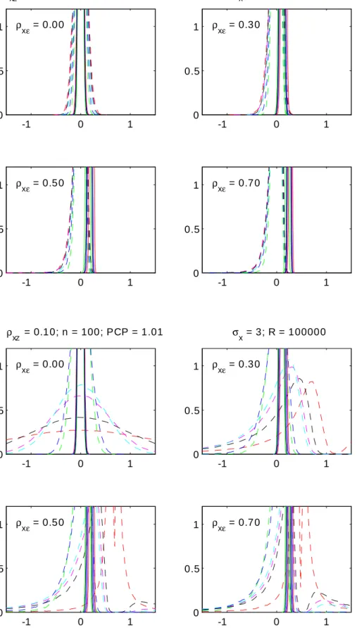
3.2. Simulated distributions
We obtained the empirical densities of OLS and IV by generating the estimators R 50;000 times and distinguishing between the sampling schemes; all series (2.1) were drawn from the
Normal distribution and we took – without loss of generality – = 0 and " = z = 1. In
all simulations we chose x = 3: This does not lead to loss of generality either, because all
depicted densities are multiples of x; which means that the form and relative positions of
the densities would not change if we changed x; the only e¤ect would be that the scale on
the horizontal axis would be di¤erent. We examined the cases x" = 0; :3; :5; :7: This gives 4
panels of densities. Most diagrams contain results for both xz =:4 and xz =:1;then the top
four panels in a diagram are those for the not so weak instrument, and the bottom four those for the much weaker instrument. Most densities are for sample size n = 100; but in some we
took n = 1000: All the relevant design parameter values and their consequences for PCP are
given in the diagrams.
Diagram 3 considers the unconditional case, so in all replications new vectors for the three series (2.1) have been drawn. The IV density is dashed (red) and the OLS density is solid (blue). The panels also show the standard asymptotic approximations for IV (dotted, red) and for OLS (dotted, blue). By not fully displaying the mode of all distributions we get a clearer picture of the tails. Even at xz = :4; where P CP = 19, the asymptotic approximation for
IV is not very accurate, especially for x" high. Although the limiting distribution is invariant for x" this is clearly not the case for the …nite sample distribution of IV. The asymptotic
approximation for the OLS distribution is so accurate that in all these drawings it collapses with the empirical distribution. For xz = :1 the standard IV approximation starts to get really bad, but it is much worse for even smaller values of xz (not depicted). For x" away
from zero OLS is clearly biased, but so is IV when the instrument is weak. In most of the panels OLS seems preferable to IV, because most of its actual probability mass is much closer to the true value of zero than is the case for IV.
Diagram 4 presents results in which thezi series has been kept …xed. Both IV and OLS are
plotted for 6 di¤erent arbitrary realizations ofzi(in the diagram indicated by 6 raw). For OLS
the densities almost coincide, except for the stronger instrument when simultaneity is serious. For IV the e¤ects of conditioning are more pronounced, especially for the stronger instrument. In Diagram 5 the same 6 realizations of the zi series have been used after stylizing them by
normalizing them such that their …rst two sample moments correspond to the population mo-ments (indicated by 6 stylized). Now all 6 curves almost coincide, and apparently the e¤ects of higher order sample moments not fully corresponding with their population counterpart has hardly any e¤ects.
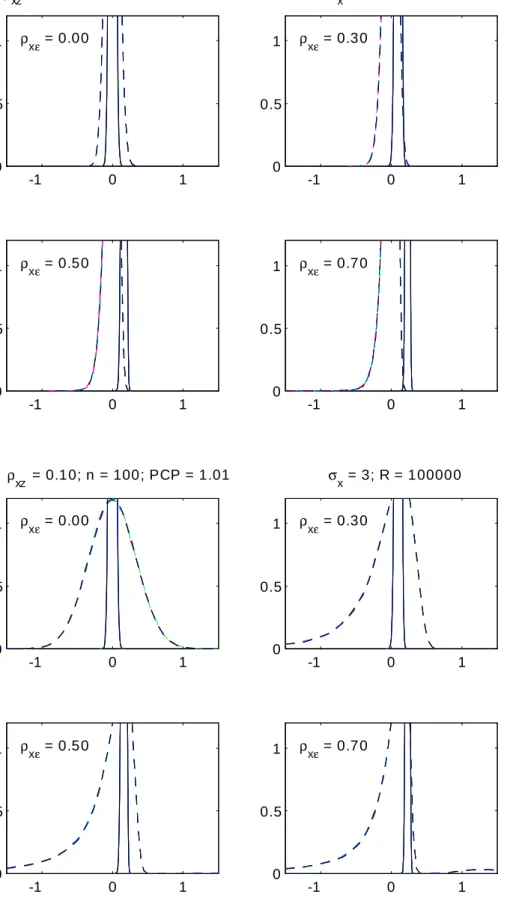
In Diagram 6 we conditioned on bothzi and vi; again using 6 arbitrary realizations. Note
that although E(zivi) = 0 the sample correlation coe¢ cientrzv may deviate from zero. The
e¤ects of this type of conditioning are much more pronounced now, just a little for OLS, but extremely so for IV in the weak instrument case. Then, the empirical distribution of IV demonstrates characteristics completely di¤erent from its standard asymptotic approximation; especially for low xz and high x" bimodality is manifest with also a region of zero density
between the two modes. Stylizing the zi and vi series (also making sure that their sample
covariance is zero) makes the curves coincide again in Diagram 7, but shows bimodality again in the case where the instrument is weak and the simultaneity serious.
From all these densities it seems obvious that the distribution of IV gets more problematic under conditioning, and that it seems worthwhile to develop a method such that OLS could be employed for inference. That this conclusion does not just pertain to very small samples can be learned from Diagram 8, where n = 1000 and xz =:1; giving rise to P CP just above 10.
The top four diagrams are unconditional, whereas the bottom four diagrams present results conditional on xi: In most cases all realizations of the OLS estimator are much closer to the
true value than most of those obtained by IV. Especially if OLS could be corrected for bias (without a major increase in variance) it would provide a welcome alternative to IV, not only when the sample is small, and even when the instrument is not all that weak.
4. Robust OLS inference under simultaneity
In Kiviet and Niemczyk (2012) an attempt was made to design inference on based on a bias corrected OLS estimator and an assumption regarding x": An infeasible version, which used
also the true values of x and " worked well, which is promising. However, after replacing x and " by sample equivalents it became clear that such a substitution at the same time
alters the limiting distribution of the bias corrected estimator, so that further re…nements of the asymptotic approximations are called for.
4.1. The limiting distribution of bias corrected OLS
We shall derive the appropriate limiting distribution in the hope that it will lead to an as-ymptotic approximation that is still reasonably accurate in …nite samples. We will focus on the unrestrained sampling scheme, because we found that the variance of OLS has a tendency to decrease by conditioning on exogenous regressors. Therefore, any resulting unconditional (regarding the exogenous variables) con…dence sets are expected to have larger coverage proba-bility (thus will be conservative) under conditioning. Moreover, when we will compare uncondi-tional robust OLS inference with uncondiuncondi-tional IV inference and the former is found to provide a useful alternative, then we would know for sure that this will certainly be the case under a restrained sampling scheme, because we have seen that conditioning worsens the situation for IV and improves it for OLS.
So, our starting point is result (b1) of Theorem 1. This suggests the unfeasible bias corrected OLS-based estimator ^U OLS( x"; "= x) ^OLS "2= 2x = ^OLS x" "= x for ; with
limiting distribution n1=2 ^U OLS( x"; "= x) d ! N 0; 2 " 2 x (1 2x") : (4.1)
This estimator is unfeasible, because it requires the values of x"and "= x:Below we shall show
that the noise-signal related quantity "= x can be estimated consistently, but this estimator
is unfeasible as well, although it just requires knowledge of the value of x" or a consistent
estimator of it. The latter would require exploiting at least one valid and relevant instrument
zi; which in its turn is a feasible procedure only when adopting the value zero for z": Since
testing the hypothesis z" = 0 is only possible by exploiting at least one other valid and
relevant instrument (which should be linearly independent from zi), we …nd ourselves in a
recursion. This highlights that making an untestable assumption is unavoidable. One either needs to adopt validity of at least one instrument, or one should adopt a particular value for
x"; provided that this would lead to an accurate and practicable inference procedure. We set
out to examine whether this is the case. Consider the estimator for
^ KLS( x") ^OLS x" 0 @^2"=(1 2x") n 1Xn i=1x 2 i 1 A 1=2 ; (4.2)
which is a function of the OLS estimator for ; the (ML) estimator for 2 given by ^2
"
n 1Xn
i=1(yi xi ^
OLS)2 and of x":We nickname this estimator KLS (kinky least-squares) for
which we …nd the following.
Theorem 2 (unconditional limiting distribution of KLS).Under Assumptions 1, 2 and 4 we have n1=2(^
KLS )! N(0; 2"= 2x):
Hence, remarkably, the standard OLS estimator, which has asymptotic variance 2
"= 2x
when x" = 0; and when x" 6= 0 has inconsistency x" "= x and – provided both " and x
have fourth moments as if they were Gaussian –the smaller unconditional asymptotic variance 2
"(1 2x")= 2x; has again the original asymptotic variance 2"= 2x after one has subtracted an
OLS-based estimate of its inconsistency based on the true value of x":To estimate the variance of ^KLS one should not use the standard expression V ard(^OLS) = ^2"=Xn
i=1x 2 i; but d V ar(^KLS) ^ 2 " (1 2 x") Xn i=1x 2 i = 1 1 2 x" d V ar(^OLS); (4.3)
because that yields plimnV ard(^KLS) = 2
"= 2x;as it should.
4.2. Simulation results on KLS-based inference
In a Monte Carlo study based on 100,000 replications we have examined the bias of both ^OLS
and ^KLS; the Monte Carlo estimate of V ar(^KLS) and the estimated expectation of its em-pirical estimateV ard(^KLS):Also we have examined the coverage probability of an asymptotic KLS based con…dence interval with nominal con…dence coe¢ cient of 95%. Hence, we analyzed the frequency over the Monte Carlo replications by which the true value of was covered by the interval
[^KLS 1:96 SDd(^KLS);^KLS+ 1:96 SDd(^KLS)]; (4.4) where both ^KLS and dSD(^KLS) (V ard(^KLS))1=2 = (1 2
x") 1=2dSD(^OLS) are calculated
on the basis of the true value of x":
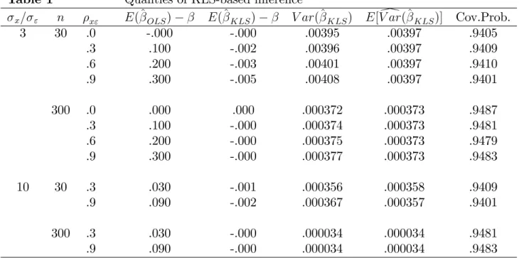
Since the simulation results in Table 1 are purely OLS based, they do not require the avail-ability of an instrumental variable, and thus instrument strength is irrelevant. No conditioning on exogenous variables occurred and all results are invariant regarding the true values of and ": Justn; x" and x= " matter, but the latter is found (and can be shown) not to a¤ect
the coverage probability of KLS con…dence intervals. The bias of OLS is found to be (almost) invariant with respect to n; and to be extremely close to the inconsistency, which predicts it to increase with (the absolute value of) x" and to be inversely related to x= ": The KLS
coe¢ cient estimator, which is based on the true value of x";is almost unbiased, and variance estimator (4.3) is found to have a minor negative bias for the true variance. The actual cov-erage probability of the KLS con…dence intervals is remarkably close to the nominal value of 95%. These estimates have a Monte Carlo standard error of about .0007, hence we establish a signi…cant slight under-coverage over all the design parameter values examined, also when
x" = 0: The latter is due to using a critical value from the normal and not from the Student
distribution. As far as the slight under-coverage is due to inaccuracies for n small in the OLS bias approximations, this could be repaired possibly by employing higher-order approximations as in Kiviet and Phillips (1996). The appearance of the factor 1 2x" in the denominator of (4.3) indicates that x" values really close to unity will be problematic.
Table 1 Qualities of KLS-based inference x= " n x" E(^OLS) E(^KLS) V ar(^KLS) E[V ard(^KLS)] Cov.Prob. 3 30 .0 -.000 -.000 .00395 .00397 .9405 .3 .100 -.002 .00396 .00397 .9409 .6 .200 -.003 .00401 .00397 .9410 .9 .300 -.005 .00408 .00397 .9401 300 .0 .000 .000 .000372 .000373 .9487 .3 .100 -.000 .000374 .000373 .9481 .6 .200 -.000 .000375 .000373 .9479 .9 .300 -.000 .000377 .000373 .9483 10 30 .3 .030 -.001 .000356 .000358 .9409 .9 .090 -.002 .000367 .000357 .9401 300 .3 .030 -.000 .000034 .000034 .9481 .9 .090 -.000 .000034 .000034 .9483
Interval (4.4) is based on standard OLS statistics only. When =2 expresses the =2 quantile of the standard Normal distribution an interval with con…dence coe¢ cient 1 is obtained by ^ OLS [(n 1=2 x" =2)=(1 2 x") 1=2]SDd(^ OLS): (4.5)
It can deviate substantially from a standard OLS interval when x"is far from zero. Its location with respect to the standard OLS interval shifts, due to the bias correction. Moreover, its width is multiplied by the factor(1 2
x") 1=2 and hence bulges up for 2x" close to unity. If one wants
to base inference on an interval assumption, say x" 2[ L
x"; Rx"];then a conservative(1 )100%
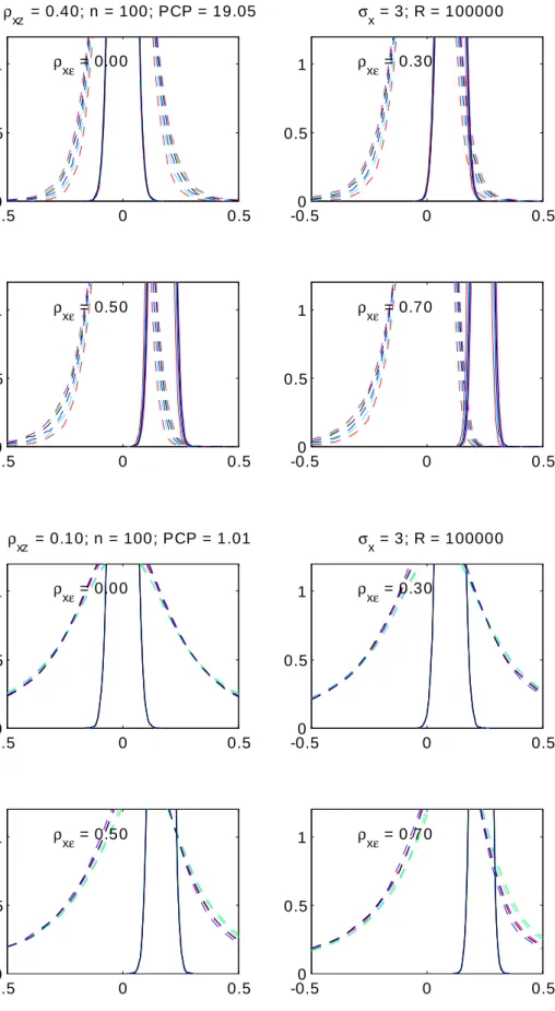
con…dence interval is obtained by taking the union of all intervals for x" in that interval. Diagrams 9 and 10 provide an impression of what such intervals might achieve in comparison to those provided by IV under ideal circumstances, namely based on the actual …nite sample distribution of IV, which in practice is very hard to approximate, whereas we have seen that this works …ne for the KLS estimator. Diagram 9 replicates the results of Diagram 3 for the …nite sample distributions of IV and OLS, but in addition it shows the densities of KLS when based on an (in)correct assumption regarding x": The blue curve uses x" = 0; so here KLS simpli…es to OLS. The other densities use the assumptions x" = :9(red), :6(green) or :3
(cyan), :3 (magenta), :6 (yellow),:9(black). Hence, in each panel at most one KLS curve uses a x" value very close to its true value (which is mentioned in the panel). The superiority of KLS when employing a x" value that is wrong by about a 0:3 margin is apparent, because
it yields a probability mass much closer to the true value of zero than IV, especially when the instrument is weak. In Diagram 10 densities of the same estimators are presented but now
for n = 1000: For a not very weak instrument and a large sample IV may do better, but for
cases where PCP is smaller than or around 10 the instrument-free KLS inference seems a very welcome alternative. This will be even more the case in practice, when the available (weak) instrument could actually be endogenous.
4.3. Comparison of the qualities of alternative con…dence sets
As already argued above, the reputation of any inference technique should be based on criteria such as: is it based on credible assumptions; does it ful…ll (also in …nite samples) its promises regarding its claimed accuracy; can it boast other credentials, such as robustness; and is its inference more e¢ cient than that produced by competing techniques. As a rule, in most contexts there does not exist a single technique which uniformly dominates all others under all relevant circumstances.
For the DGP examined above we will now compare the properties of various con…dence sets on the scalar parameter : We will examine KLS-based con…dence sets with IV-based con…dence sets, where the latter are constructed from either the standard asymptotic Wald (W) test statistic or by inversion of the Anderson-Rubin (AR) statistic. The W procedure is known to be defective when instruments are weak, whereas the AR procedure is known to be robust under the null when instruments are weak. Mikusheva (2010) claims that it performs reasonably well amongst other techniques which focus on invariance of the asymptotic null distribution with respect to weakness of instruments. However, in the present just identi…ed case these other (LM and LR based) techniques simplify to the AR procedure.
In the present context, the Wald statistic for H0 : = 0 is given by
W( 0) = ^ IV 0 d SD(^IV) !2 ; with dSD(^IV) = (y x ^ IV)0(y x^IV)=(n 1) x0z(z0z) 1z0x !1=2 ; (4.6)
where y; xand z aren 1vectors containing all the sample data. For nominal(1 ) 100% con…dence coe¢ cient, it yields con…dence interval
^
IV + =2dSD(^IV);^IV + 1 =2SDd(^IV) : (4.7)
The AR test statistic for the same hypothesis is performed by substituting the reduced form equation in the structural form relationship and next testing the signi…cance of the slope in the equation y x 0 =z ( 0) +"+ ( 0)v: Under the null the tests statistic
AR( 0) = (n 1) (y x 0) 0z(z0z) 1z0(y x 0) (y x 0)0[I z(z0z) 1z0](y x 0) (4.8) is asymptotically distributed as 2(1) and under normality exactly as F(1; n 1): It implies the con…dence interval
CAR( ) =f 0 :AR( 0)< F (1; n 1)g: (4.9)
This can be established by solvinga 2+b +c 0;wherea =x0Ax; b= 2x0Ayandc=y0Ay;
with A=I dz(z0z) 1z0 andd= 1 + (n 1)=F (1; n 1):If =b2 4ac 0then an interval
follows easily provided a 0;when a >0; though, the interval consists of the whole real line, except for a …nite interval, and thus has in…nite length. When < 0 the interval is empty for a < 0 and equals the full real line when a >0 (note that <0 and a = 0 cannot occur). These anomalies, if they really do occur, would be the result of uncomfortable behavior of the AR statistic under the alternative hypothesis, implying either unit rejection probability for all alternatives (CI empty), or zero rejection probability for either all alternatives (CI is the full real line) or for just a closed set of alternatives (CI is the real line, except for a particular interval). In the simulations to follow, we will monitor the occurrence of these anomalies.
Since we will focus on the width of the interval, we will examine the 0 and a 0 cases exclusively, in order to exclude non-existing intervals and intervals of in…nite length. For those with …nite length we will report the median width, because the occurrence of outliers clearly indicates that for both W and AR the random variable width has no …nite moments.
Regarding the KLS-based intervals we will present results for three intervals [ L x"; Ux"];
namely: (A) Lx" = Ux" = x"; (B) Lx" = x" 0:2; Ux" = x"+ 0:2; and (C) x"L = 0; Ux" = 0:5:
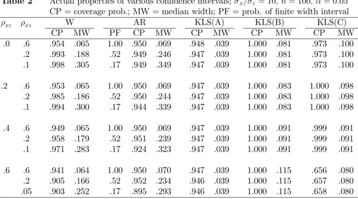
Of course, in practice it will be unrealistic that one could ever attain (A), and although (B) is more realistic, in practice one might specify occasionally an interval that excludes the true value. This is possible with interval (C), which simply states that any simultaneity will be non-negative and not exceeding0:5:We ran 100,000 replications for a few combinations of x" and xz values forn= 100;giving rise to PCP values equal to 56.25, 4.16 and 1.01 respectively.
Table 2 Actual properties of various con…dence intervals; x= " = 10; n= 100; = 0:05
CP = coverage prob.; MW = median width; PF = prob. of …nite width interval
x" xz W AR KLS(A) KLS(B) KLS(C) CP MW PF CP MW CP MW CP MW CP MW .0 .6 .954 .065 1.00 .950 .069 .948 .039 1.000 .081 .973 .100 .2 .993 .188 .52 .949 .246 .947 .039 1.000 .081 .973 .100 .1 .998 .305 .17 .949 .349 .947 .039 1.000 .081 .973 .100 .2 .6 .953 .065 1.00 .950 .069 .947 .039 1.000 .083 1.000 .098 .2 .985 .186 .52 .950 .244 .947 .039 1.000 .083 1.000 .098 .1 .994 .300 .17 .944 .339 .947 .039 1.000 .083 1.000 .098 .4 .6 .949 .065 1.00 .950 .069 .947 .039 1.000 .091 .999 .091 .2 .958 .179 .52 .951 .239 .947 .039 1.000 .091 .999 .091 .1 .971 .283 .17 .924 .323 .947 .039 1.000 .091 .999 .091 .6 .6 .941 .064 1.00 .950 .070 .947 .039 1.000 .115 .656 .080 .2 .905 .166 .52 .952 .234 .946 .039 1.000 .115 .657 .080 .05 .903 .252 .17 .895 .293 .946 .039 1.000 .115 .658 .080
Table 2 shows that for a weak instrument the IV-based Wald test can both be conservative (when the simultaneity is moderate) and yield under-coverage (when the simultaneity is more serious). The AR procedure is of little practical use in this model, because it does not improve on the Wald test when the latter works well, and although it does produce intervals with appropriate coverage when the instrument is weak, much too frequently it does not deliver an interval (of …nite length) at all. Moreover, the few intervals that it delivers when xz =:1have
larger width on average than those produced by the Wald procedure, even when the latter are conservative. The KLS(A) procedure performs close to perfect. Its coverage is not only very close to 95%, but its performance is also invariant with respect to both x" and zx; and the
width of the interval is 60% (for xz =:6) or just about 15% (for xz =:1) of the Wald interval. The more realistic KLS(B) intervals are much too conservative, but nevertheless have smaller width than the Wald intervals when the instrument is weak. The same holds for the realistic KLS(C) intervals, provided that the true value of x" is in the interval. If this is not the case, then the KLS procedure breaks down.
4.4. Empirical illustration
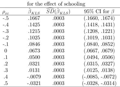
The application that has undoubtedly received most attention over the last two decades in the debate and research on the e¤ects of weakness and validity of instruments on the coe¢ cient estimate of an endogenous variable is Angrist and Krueger (1991), who analyzed the returns to schooling on log wage. In Donald and Newey (2001) and Flores-Lagunes (2007) many variants of IV based estimates have been obtained. Donald and Newey (2001, p.1178) present also the OLS results for the coe¢ cient estimate for schooling, being .0673 with a standard error equal to .0003. This has been obtained from a sample of size 329500. They also indicate sample second moments of the structural and reduced form disturbances which suggest estimates of the simultaneity coe¢ cient equal to -.127, -.192 and -.204 according to 2SLS, LIML and B2SLS respectively. However, when the IV estimates are biased or even inconsistent due to the use of invalid or weak instruments these assessments may be misleading. From the OLS estimates we can deduce for di¤erent assumptions on x" the KLS inferences collected in Table 3.
Table 3 KLS estimates and con…dence intervals for the e¤ect of schooling
x" ^KLS SDd(^KLS) 95% CI for -.5 .1667 .0003 (.1660, .1674) -.4 .1425 .0003 (.1418, .1431) -.3 .1215 .0003 (.1208, .1221) -.2 .1025 .0003 (.1019, .1031) -.1 .0846 .0003 (.0840, .0852) 0 .0673 .0003 (.0667, .0679) .1 .0500 .0003 (.0494, .0506) .2 .0321 .0003 (.0315, .0327) .3 .0131 .0003 (.0125, .0138) .4 -.0079 .0003 (-.0085, -.0072) .5 -.0321 .0003 (-.0328, -.0314)
Note that unlike the IV results the KLS inferences are not a¤ected by the quality or validity of any of the external instrumental variables. However, like the IV results, they do assume that apart from the schooling variable all the partialled out regressors are exogenous. We …nd that when x" were close to -.2 indeed, KLS infers that the e¤ects of schooling are close to .10 and in fact much closer than IV is able to produce. The IV-based techniques examined in Flores-Lagunes (2007) yield much wider con…dence intervals of about [:8; :13]: From KLS one can deduce that such values are plausible only if x" is in the range (-.35,-.08). If x" is in fact mildly positive (as many have argued on theoretical grounds), then the e¤ect of schooling on wage is actually much smaller than .10 and possibly just around .03 as Table 3 shows. Then the present IV …ndings would be the result of their inescapable frailty when instruments are weak or even invalid.
5. Conclusions
It is well-known now that the actual distribution of IV estimators gets rather anomalous when based on weak instruments. This paper shows that another factor causing serious deviations of
the …nite sample distribution of IV from its standard asymptotic approximation is the sampling scheme. Conditioning on exogenous regressors aggravates the anomalies of IV. It leads more often to the occurrence of bimodality and occasionally to an area close to the median of the distribution where the density is zero. On the other hand, the distribution of the OLS estimator in simultaneous equations is much smoother, always unimodal and much less dispersed than for IV, it is much less a¤ected by the sampling scheme and its asymptotic approximation is remarkably accurate even in small samples. Its major problem is its inconsistency, although this is bounded. We demonstrate how the OLS estimator can be corrected to render it consistent, without using instrumental variables at all. According to the established view, however, this corrected estimator is unfeasible, because it is based on an unknown parameter, namely the degree of simultaneity. But in fact similar problems a- ict the single equation IV estimator, because its consistency is also based on making assumptions on parameter values, namely the coe¢ cient values (possibly their exclusion) of at least as many regressors as the relationship involves endogenous regressors with unknown coe¢ cients. Only a surplus of such restrictions and corresponding orthogonality conditions can be veri…ed by empirical-statistical methods; an initial set as large as the number of included endogenous regressors requires parameter values chosen on the basis of rhetorical arguments to be deduced from economic theory or natural experiment settings. Even when these adopted restrictions are valid we show how vulnerable IV inferences are when instruments are weak. To be able to avoid this situation we derive the limiting distribution of bias corrected OLS, which allows to produce inference on the structural coe¢ cient for a range of possible values of the simultaneity parameter. By taking the union of a series of con…dence intervals we obtain relatively e¢ cient, accurate, robust and often more credible inferences, without the need to nominate instrumental variables. In future research we plan to generalize the method for models under less strict independence restrictions involving more than just one endogenous regressor from which exogenous regressors are not necessarily partialled out in order to construct accurate external-instrument-free inference for all structural coe¢ cients.
References
Andrews, D.W.K., Stock, J.H., 2007a. Inference with Weak Instruments, Chapter 6 in: Blundell, R., Newey, W.K., Persson, T. (eds.), Advances in Economics and Econometrics, Theory and Applications, 9th Congress of the Econometric Society, Vol. 3. Cambridge, UK: Cambridge University Press.
Andrews, D.W.K., Stock, J.H., 2007b. Testing with many weak instruments. Journal of Econometrics 138, 24-46.
Angrist, J.D., Krueger, A.B., 1991. Does compulsory school attendance a¤ect schooling and earnings? Quarterly Journal of Economics 106, 979-1014.
Angrist, J.D., Pischke, J-S., 2010. The credibility revolution in empirical economics: How better research design is taking the con out of econometrics. Journal of Economic Perspectives
24, 3-30.
Conley, T.G., Hansen, C.B., Rossi, P.E., 2012. Plausibly exogenous. The Review of Eco-nomics and Statistics 94, 260-272.
Donald, S.G., Newey, W., 2001. Choosing the number of instruments. Econometrica 69, 1161-1191.
Erickson, T., 1993. Restricting regression slopes in the errors-in-variables model by bound-ing the error correlation. Econometrica 61, 959-969.
Flores-Lagunes, A., 2007. Finite sample evidence of IV estimators under weak instruments.
Journal of Applied Econometrics 22, 677-694.
Forchini, G., 2006. On the bimodality of the exact distribution of the TSLS estimator.
Econometric Theory 22, 932-946.
Goldberger, A.S., 1964. Econometric Theory. John Wiley & Sons. New York.
Hahn, J., Hausman, J.A., 2003. Weak instruments: Diagnosis and cures in empirical econometrics. American Economic Review 93, 181-125.
Hausman, J.A., 1978. Speci…cation tests in econometrics. Econometrica 46, 1251-1271. Hu, Y., 2006. Bounding parameters in a linear regression model with a mismeasured regressor using additional information. Journal of Econometrics 133, 51-70.
Hillier, G., 2006. Yet more on the exact properties of IV estimators. Econometric Theory
22, 913-931.
Kapteyn, A., Wansbeek, T., 1984. Errors in variables: Consistent Adjusted Least Squares (CALS) estimation. Communications in Statistics: Theory and Methods 13, 1811-1837.
Kiviet, J.F., Niemczyk, J., 2007. The asymptotic and …nite sample distribution of OLS and simple IV in simultaneous equations. Journal of Computational Statistics and Data Analysis
51, 3296-3318.
Kiviet, J.F., Niemczyk, J., 2012. The asymptotic and …nite sample (un)conditional distri-butions of OLS and simple IV in simultaneous equations. Journal of Computational Statistics and Data Analysis 56, 3567-3586.
Kiviet, J.F., Phillips, G.D.A., 1996. The bias of the ordinary least squares estimator in simultaneous equation models. Economics Letters 53, 161-167.
Kraay, A., 2012. Instrumental variables regressions with uncertain exclusion restrictions: A Bayesian approach. Journal of Applied Econometrics 27, 108-128.
Maddala, G.S., Jeong, J., 1992. On the exact small sample distribution of the instrumental variable estimator. Econometrica 60, 181-183.
Manski, C.F., 2003. Partial Identi…cation of Probability Distributions. New York, Springer. Manski, C.F., 2007. Identi…cation for Prediction and Decision. Cambridge, MA. Harvard University Press.
Manski, C.F., Pepper, J.V., 2000. Monotone instrumental variables: With an application to the demand for schooling. Econometrica 68, 997-1010.
Manski, C.F., Pepper, J.V., 2009. More on monotone instrumental variables. Econometrics Journal 12, S200-S216.
Mariano, R.S., 1973. Approximations to the distribution functions of the ordinary least-squares and two-stage least-least-squares estimators in the case of two included endogenous variables.
Econometrica 41, 67-77.
Mikusheva, A., 2010. Robust con…dence sets in the presence of weak instruments. Journal of Econometrics 157, 236-247.
Nelson, C.R., Startz, R., 1990a. Some further results on the exact small sample properties of the instrumental variable estimator. Econometrica 58, 967-976.
Nelson, C.R., Startz, R., 1990b. The distribution of the instrumental variables estimator and its t-ratio when the instrument is a poor one. Journal of Business 63, S125-S140.
Nevo, A., Rosen, A.M., 2012. Identi…cation with imperfect instruments. To appear in: The Review of Economics and Statistics.
Phillips, P.C.B., 1983. Exact small sample theory in the simultaneous equations model. In M.D. Intriligator, Z. Griliches (eds.), Handbook of Econometrics, Ch. 8, 449-516. North– Holland.
Phillips, P.C.B., 1989. Partially identi…ed econometric models. Econometric Theory 5, 181-240.
Phillips, P.C.B., 2006. A remark on bimodality and weak instrumentation in structural equation estimation. Econometric Theory 22, 947–960.
Phillips, P.C.B., 2009. Exact distribution theory in structural estimation with an identity.
Econometric Theory 25, 958-984.
Rothenberg, T.J., 1972. The asymptotic distribution of the least squares estimator in the errors in variables model. Unpublished mimeo.
Sawa, T., 1969. The exact sampling distribution of ordinary least squares and tw0-stage least squares estimators. Journal of the American Statistical Association 64, 923-937.
Schneeweiss, H., 1980. Di¤erent asymptotic variances for the same estimator in a regression with errors in the variables. Methods of Operations Research 36, 249-269.
Staiger, D., Stock, J.H., 1997. Instrumental variables regression with weak instruments.
Econometrica 65, 557-586.
Tamer, E., 2010. Partial identi…cation in econometrics. Annual Reviews Economics 2, 167-195.
Woglom, G., 2001. More results on the exact small sample properties of the instrumental variable estimator. Econometrica 69, 1381-1389.
Appendices
A. The relevance of conditioning on unobserved variables
The DGP introduced in section 2.1 with just three fundamental parameters can of course easily be generalized in various directions. We will indicate here one particular type of possible extension, just because that supports the interpretation of the component vi of the reduced form disturbance vi and provides arguments to examine in Monte Carlo experiments both
cases wherevi is either random or …xed. When allowing for overidenti…cation, this requires to replacezi IID(0;1)by theL >1seriesz
(l)
i IID(0;1); l = 1; :::; L: Then the reduced form
equation generalizes to xi = XL l=1 lz (l) i +vi; (A.1)
where again vi =vi + "i: Without loss of generality we may assume that the L instruments
(possibly after a transformation) are all mutually independent. Then it follows that 2 x = XL l=1 2 l + 2 + 2v : (A.2) With E(xiz (l) i ) = xz(l) x = l and (2.10) one …nds 2v = 2x(1 2x" XL l=1 2 xz(l)): This
again implies admissibility restrictions, which here involve an (L+ 1)-dimensional unit sphere, namely 2 x"+ 2 xz(1) +:::+ 2 xz(L) 1: (A.3)
Now imagine that a researcher has available (or is aware of) only L# of the instrumental variables, namely zi(l) for l= 1; :::; L#; where0< L#< L: Then xi = 1zi(1)+:::+ L#z(L
#) i + vi# +vi + "i;with vi# = L#+1z (L#+1) i +:::+ Lz (L) i :Nowv #
i +vi plays the role of the earlier
vi:Actual inference can now only be conditioned on theL# available instruments. Thus, in a Monte Carlo analysis of that situation one may choose to keep only theseL#instruments …xed. However, it does make sense too to keep vi# …xed as well, simply if one is of the opinion that this mimics the actual population better. Keeping both vi# andvi …xed simply represents the extreme case in which all the contributions to xi which are exogenous with respect to "i but
are not explicitly taken into account by the available instruments, are supposed to represent the actual population of interest best. For our simple model where L = 1 there are no such intermediary cases for conditioning on justL# instruments, but only the two extremesCz and
Cx :
B. Proofs
Lemma: From D 1 = [D+ (D D)] 1 =D 1(1 +D 1D~) 1;where D 1D~ =O
p(n 1=2); the
Taylor expansion (1 + D 1D~) 1 = 1 D 1D~ +o
p(n 1=2) yields D 1 = D 1(1 D 1D~) +
op(n 3=2); giving R = N=D = (N + ~N)D 1(1 D 1D~) +op(n 1=2): Note that N D~ 2D~ =
Op(n 1): So, conditional onC, we have
n1=2(R N =D) = (D=n) 1n 1=2[ ~N (N =D) ~D] +op(1):
Now the result of the lemma follows directly by omitting the remainder term and invoking standard results attributed to Slutsky and Cramér to the right-hand term.
Theorem 1:
For obtaining the unconditional limiting distribution of IV we do not need the Lemma, and can just follow the standard textbook approach. This exploits that according to the Law of Large Numbers (LLN) plimn 1Pn
i=1zixi = xz 6= 0; while a standard Central Limit Theorem (CLT) yields n 1=2Pn i=1zi"i d ! N(0; 2 " 2z); since E(zi"i) = 0; E(zizj"i"j) = 0 for i 6= j and E(z2
i"2i) = 2" 2z; because of the the independence of zi and "i: Then it follows
from (3.1) that n1=2(^ IV ) = (n 1 Pn i=1zixi) 1 n 1=2Pn i=1zi"i d ! N (0; 2 " 2z= 2xz); where 2 z= 2xz = 1=( 2xz 2x):
When conditioning ^IV on the zi we employ the Lemma with N = Pni=1zi"i and D = Pn i=1zixi and …nd N E(N j Cz) = E(Pni=1zi"i j Cz) =Pni=1ziE("i j Cz) = 0; ~ N N N =Pni=1zi"i; with N~ j Cz =Op(n1=2); D E(Dj Cz) = E( Pn i=1zixi j Cz) = Pn i=1ziE(xi j Cz) = Pn i=1z 2 i =O(n); ~ D D D=Pni=1zi(xi zi) = Pn i=1zivi; with D~ j Cz =Op(n1=2):
We conclude that N~ j Cz =Op(n1=2); because V ar(Pni=1zi"i j Cz) = 2" Pn
i=1z 2
i = O(n): The
result for D follows immediately from (2.3), whereas D~ j Cz = Op(n1=2); because we …nd
V ar(Pni=1zivi j Cz) = 2v Pn
i=1z 2
i = O(n): Hence, the conditions of the Lemma are satis…ed,
although N is actually much smaller than O(n): Moreover, N~ ND=D~ = ~N = Pni=1zi"i;
thus n 1=2( ~N ND=D~ ) = n 1=2Pn
i=1zi"i; for which we have already obtained that it has conditional expectation zero and conditional variance 2"n1
Pn i=1z
2
i;thus a standard CLT yields
V0 = lim 2"n1 Pn
i=1z 2
i = 2" 2z:SincelimD=n= 2z = xz z xwe …nd that conditioning on the
instruments has no e¤ect. This is because N = 0 and due to limn 1D= lim 1
n Pn i=1E(zixi j zi) = limn1 Pn i=1z 2 i = 2z = plimn1 Pn i=1zixi:
Conditioning IV on xi and exploitingE(xi"i) = 0 yields
N E(N j Cx ) =E( Pn i=1zi"i j Cx ) = Pn i=1ziE("i j Cx ) = 0; ~ N N N =Pni=1zi"i; with N~ j Cx =Op(n1=2); D E(Dj Cx ) = E[ Pn i=1zi(xi + "i)j Cx ] = Pn i=1zixi = Pn i=1z 2 i + Pn i=1zivi =O(n); ~ D D D =Pni=1zi(xi zi vi) = Pn i=1zi"i; with D~ j Cx =Op(n 1=2): That N~ j Cx = Op(n1=2) is now self-evident. Because V ar( Pni=1zi"i j Cx ) = 2"
Pn i=1z 2 i = O(n) we …nd D~ j Cx =Op(n1=2): Again N = 0; giving n 1=2( ~N ND=D~ ) = n 1=2Pni=1zi"i and V0 = lim 2" 1 n Pn
i=1zi2 = 2" 2z: Because limD=n = 2z + lim 2"
1
n Pn
i=1E(zivi) = 2z = xz z x;we again …nd the same limiting distribution, and hence have established result (a) of
the Theorem.
For simple OLS we have N =Pni=1xi"i and D= Pn
i=1x2i: ForC empty and using
decom-position xi = zi+vi + "i =xi + "i we easily obtain
N = E(Pni=1xi"i) = n 2" =O(n); ~ N = Pni=1(xi"i 2") = Pn i=1[xi"i+ ("2i 2 ")] =Op(n1=2); D = E(Pni=1xi2) =n 2x =O(n); ~ D = Pni=1(x2i x2) = Op(n1=2);
where the orders of probability of N~ and D~ follow because their expectation is zero and their variance is O(n); provided xi and "i have …nite 4th moments, which is the case under