Exploratory Trading
Adam D. Clark-Joseph
∗September 10, 2013
Abstract
Using comprehensive, account-labeled message records from the E-mini S&P 500 futures mar-ket, I examine the mechanisms that enable high-frequency traders (HFTs) to protably anticipate price movements. HFTs in my sample consistently lose money on numerous small orders, then earn high prots on larger orders, and I model how a trader could use her own small, exploratory orders to gather valuable, private information. Direct empirical tests of the model's predictions support the hypothesis that HFTs use this sort of exploratory trading to actively learn about likely future price movements.
∗University of Illinois Urbana-Champaign, E-mail: [email protected]. I thank Celso Brunetti, Richard Haynes, Andrei
Kirilenko, Todd Prono, Tugkan Tuzun, Brian Weller and Steve Yang for their assistance with the empirical component of this paper, and I thank John Campbell, Brock Mendel, Andrei Shleifer, Alp Simsek and Jeremy Stein for their invaluable advice and comments. I thank seminar participants at Harvard, UBC Sauder, Indiana Kelley, Stanford GSB, Illinois, OSU Fisher, Dartmouth Tuck, Wharton, and the NYU Stern Microstructure Meeting for their useful feedback, and I thank Terrence Hendershott for his insightful discussion. I gratefully acknowledge the support of an NSF Graduate Research Fellowship. The views expressed in this paper are my own and do not constitute an ocial position of the Commodity Futures Trading Commission, its Commissioners, or sta.
1 Introduction
Automation pervades modern nancial markets, and trading responsibilities that once fell on human agents have been delegated increasingly to computer algorithms. Much of the algorithmic activity in major markets emanates from so-called high-frequency traders (HFTs). Although it dominates modern nancial exchanges, HFTs' activity remains largely mysterious and opaqueit is the dark matter of the trading universe.
The prominence, novelty, and opacity of HFTs' activity has fueled heated public controversy about the desirability of high-frequency trading. Advocates assert that HFTs improve price discovery, liquidity, and market resilience. Critics contend that HFTs make no unique contribution to price discovery, provide only illusory liquidity, harm traditional market participants, and increase market fragility. This debate has sparked a variety of proposals for policies to regulate or deter high-frequency trading, and a few proposed policies have begun to be adopted. However, the impact of high-frequency trading on dierent aspects of market quality and on the welfare of non-HFT market participants is not well understood.
Understanding and explaining the impacts of high-frequency trading requires knowledge of why and how HFTs' strategies work, as does the counterfactual analysis necessary for optimal policy design. To this end, the present paper analyzes economic underpinnings of HFTs' strategies in the context of the market for the E-mini Standard & Poors 500 stock index futures contract (henceforth, E-mini). I
nd that HFTs in the E-mini market earn roughly40%of their prots from the transactions that they
initiatethat is, from their so-called aggressive ordersand I examine the mechanism underlying HFTs' capacity to earn these prots.
1.1 Empirical Research on High-Frequency Training
The archetypal HFT generates a large number of trades, but this eponymous high trading frequency is only one of several traits that characterize HFTs. Two further hallmarks of HFTs are their extremely short time-frames for maintaining positions, and their propensity to end the trading day holding at most minimal net inventory positions. HFTs are also characterized by their ability to react to market events with only a tiny delay, or latency, typically on the order of milliseconds.
Empirical study of high-frequency trading has proven challenging, but not impossible. For ex-ample, Brogaard et al. (2012) obtain and analyze a NASDAQ dataset that ags messages from an
aggregated group of 26 HFT rms, and Hasbrouck and Saar (2011) conduct a complementary analysis by statistically reconstructing strategic runs of linked messages in public NASDAQ data. Both of these studies suggest benecial eects from HFTs' activity, in line with the ndings for general algo-rithmic trading by Hendershott et al. (2011) and Hendershott and Riordan (2009); however, inherent limitations of the underlying data restrict these studies' scope to explain how and why such eects arise. Empirical results in Baron et al. (2012), Hagströmer and Nordén (2013), and the present paper indicate that HFTs exhibit considerable heterogeneityeven in a market for a single asset. As a result, aggregate HFT activity reveals little about what individual HFTs really do.
Data suitable for the study of individual HFTs' activity are dicult to obtain. Whereas publicly available 13-F forms reveal the behavior of institutional investors at a quarterly frequency, there is no comparable public data that can be used to track and analyze the behavior of individual traders at a second- or millisecond-frequency. The only fully adequate data available for academic research on high-frequency trading in U.S. markets come from regulatory records that the Chicago Mercantile Exchange provides to the U.S. Commodity Futures Trading Commission. Kirilenko et al. (2010) pioneered the use of transaction data from these records to investigate high-frequency trading in the E-mini market during the so-called Flash Crash of May 6, 2010. This work introduced a data-driven scheme to classify trading accounts using simple measures of overall trading activity, intraday variation in net inventory position, and inter-day changes in net inventory position. Of the accounts with suciently small intra- and inter-day variation in net position, Kirilenko et al. classify those with the highest levels of trading activity as HFTs, and these accounts are quintessential high-frequency traders.
Kirilenko et al. nd that HFTs participate in over one-third of the trading volume in the E-mini market, and subsequent research by Baron et al. (2012) documents the large and stable prots that HFTs in the E-mini market earn. This work provides empirical conrmation of HFTs' importance, and it oers some crisp descriptions of HFTs' activity. However, it does not attempt to explain why HFTs act as they do, or how HFTs earn prots. Indeed, no extant empirical research attempts such explanations.
In this paper, I address a central aspect of this open problem, namely the question of how HFTs in the E-mini market earn prots on their aggressive orders. When a trader executes an aggressive order, he pays his counterparty a fraction of the bid-ask spread, so the trader must correctly anticipate a price movement to prot from his aggressive order. If a trader prots on an aggressive order, the
standard explanation is that he was trading on some private information. However, since the sources of private information available to HFTs are unclear, this standard explanation of aggressive trading prots simply raises the new question of how HFTs might obtain valuable private information.
1.2 Active Learning, Exploration, and Private Information
How do HFTs in the E-mini market make money from their aggressive orders? One possibility is that HFTs merely react to public information faster than everyone else; this premise underlies the models of Jarrow and Protter (2011), Cespa and Foucault (2008), and Biais et al. (2010). A second possibility is that HFTs simply front-run coming demand when they can predict future aggressive orders. HFTs can react to public information faster than some other market participants, and I nd that many HFTs do trade ahead of predictable future aggressive orders at certain times, consistent Hirschey's (2011) results from NASDAQ data. However, I nd evidence that the HFTs who prot on average from their aggressive orders also do something more to obtain private information: they use a form of active learning. The concept of active learning in nancial markets dates back at least to the work of Leach and Madhavan (1992) and (1993), so these HFTs are not doing something completely novel, but rather are using a new incarnation of an old idea.
I identify the HFTs who prot from their aggressive orders, then I investigate how they manage to do this. I show that the HFTs who prot from their aggressive trading use small aggressive orders to obtain private information about the price-elasticity of supply, which helps to forecast the price-impact
of predictable demand innovations.1 Demand innovations in the E-mini market are easy to predict,
but the price-elasticity of supply is not, and price-impact is usually too small for indiscriminate front-running of predictable demand to be protable. However, the private information about price-impact that an HFT's small aggressive orders generate enables the HFT to trade ahead of predictable demand at only those times when it is protable to do so, i.e., when price-impact is large. To elucidate how this active-learning process works, I develop a theoretical model of what I term exploratory trading. Fundamentally, the model of exploratory trading rests on the notion that an HFT's aggressive orders generate valuable private information, specically, information about the price-impact of the aggressive orders that may follow. When an HFT places an exploratory order and observes a large 1To be more precise, the market response to these small aggressive orders provides private information about the
dynamic behavior of passive orders resting in the orderbook (which is analogous to supply elasticity). This information helps to forecast the price-impact of future aggressive order-ow (which is analogous to demand innovations). The labels supply and demand are merely heuristics in the context of the market for E-mini contracts, but they are rigorously accurate in the context of the market for liquidity/immediacy.
price-impact, he learns that supply is temporarily inelastic. If the HFT knows that there is going to be more demand soon thereafter, he can place a larger order (even with a high price-impact) knowing that the price-impact from the coming demand will drive prices up further and ultimately enable him to sell at a premium that exceeds the price-impact of his unwinding order. When an HFT knows that supply is temporarily inelastic, he follows a routine demand-anticipation strategy. The purpose of exploratory trading is not to learn about future demand, but rather to identify the times at which trading in front of future demand will be protable. In section 2, I present a model to formalize the concept of exploratory trading, and I derive the model's central testable predictions, which provide the blueprint for my empirical analysis.
Using novel electronic message data at the Commodity Futures Trading Commission, I examine the protability of individual HFTs' aggressive orders. I nd that eight of the 30 HFTs in my sample prot from their aggressive trading overall and signicantly outperform non-HFTs. However, these same eight HFTs all lose money on their smallest aggressive orders. (For brevity, I refer to these eight HFTs as A-HFTs, and to the remaining 22 as B-HFTs.) Exploratory trading would produce just such a pattern of incurring small losses on exploratory orders then realizing large gains; these descriptive results both motivate further tests and suggest the A-HFTs' small aggressive orders as natural candidates for potential exploratory orders.
To explicitly test the predictions of the exploratory trading model for the eight A-HFTs, I rst examine the extent to which information about the changes in the orderbook following small ag-gressive orders explains the prots that various traders earn on subsequent agag-gressive orders. The exploratory trading model predicts that the changes following an A-HFT's small aggressive order provide information that will explain a signicant additional component of the A-HFT's subsequent performance, but that this information will not explain any additional component of other traders' subsequent performance. Consistent with these two predictions, I nd that the orderbook changes im-mediately following A-HFTs' small aggressive orders provide signicant additional explanatory power for the respective A-HFTs' performance on their larger aggressive orders, but not for other traders' performance. I next test the prediction that the private information from the orderbook response to a given A-HFT's small aggressive orders helps to explain the incidence of subsequent larger aggressive orders, in addition to explaining those orders' performance. This third prediction, too, is borne out empirically. Finally, to assess the practical importance and potential value of exploratory information, I construct a simple, purely aggressive trading strategy based strictly upon public information, then I
construct additional trading strategies that augment the public-information strategy with crude forms of exploratory information. Using market data, I simulate the performance of these strategies and nd that incorporating exploratory information improves strategy performance dramatically, and indeed delivers simulated performance sucient to earn positive prots from aggressive trading.
The remainder of this paper is organized as follows: Section 2 presents a simple model of ex-ploratory trading, along with the model's central predictions, and establishes the empirical agenda. Section 3 describes the dataset, presents some summary statistics, and precisely denes HFTs. Section 4 addresses the overall protability of HFTs' aggressive orders and precisely characterizes the A-HFTs, then examines the A-HFTs' losses on small aggressive orders. Section 5 presents direct empirical tests of the exploratory trading model's key predictions, and section 6 examines the practical signicance of exploratory information. Section 7 discusses extensions and implications of the empirical results. Section 8 concludes.
2 Exploratory Trading: Theory
As noted in the introduction, demand innovations in the E-mini market are easy to predict from public market data, but the price-elasticity of supply is not. Although there are times when supply is unaccommodating and high future demand forecasts price changes that are large enough to prot from, such times are dicult or impossible to identify using only passively gathered public market data. In this type of setting, a trader can obtain additional information about supply conditions by placing an exploratory aggressive order and observing how prices and supply respond. The additional exploratory information enables the trader to determine whether supply is accommodating (and expected price-impact small) or unaccommodating (and expected price-impact large), and this helps the trader to decide whether he can prot by trading ahead of an imminent demand innovation. To codify the intuitions above, I use a two-period model with two possible states for supply conditions (accommodating or unaccommodating), and three possible demand innovations in the second period (positive, negative, or zero). This model should be interpreted as a single instance of the hundreds or thousands of similar scenarios that arise throughout the trading day. To model a market in which demand is easy to predict, but supply elasticity is not, I assume that the demand innovation is automatically revealed before it arrives in the second period, but the state of supply conditions is only revealed if a trader places an aggressive order in the rst period.
I consider the problem facing a single trader, the HFT. In the rst period, the HFT has the opportunity to place an aggressive order and thereby learn about supply conditions. In the second period, regardless of what happened in the rst period, the HFT observes a signal about future demand, after which he again has an opportunity to place an aggressive order. The signal of future demand forecasts price innovations much more accurately when combined with information about supply conditions than it does when used on its own. If the HFT places an aggressive order in the rst period, he eectively buys supply information that he can use in the second period to better decide whether he should place another aggressive order.
The rest of this section is devoted to formally developing a model of exploratory trading and extracting the model's key testable predictions. Appendix A contains full mathematical details.
2.1 Preliminaries
In an order-driven market, every regular transaction is initiated by one of the two executing transac-tors. The transactor who initiates is referred to as the aggressor, while the opposite transactor is referred to as the passor. The passor's order was resting in the orderbook, and the aggressor entered a new order that executed against the passor's preexisting resting order. Assuming that prices are discrete, the lowest price of any resting sell order in the orderbook (best ask) always exceeds the highest price of any resting buy order in the book (best bid) by at least one increment (the minimal price increments are called ticks). A transaction initiated by the seller executes at the best bid, while a transaction initiated by the buyer executes at the best ask; the resulting variation in trans-action prices between aggressive buys and aggressive sells is known as bid-ask bounce. Hereafter, except where otherwise noted, I will restrict attention to price changes distinct from bid-ask bounce. Empirically, the best ask for the most actively traded E-mini contract almost always exceeds the best bid by exactly one tick during regular trading hours, so movements of the best bid, best ask, and mid-point prices are essentially interchangeable.
If the best bid and best ask were held xed, a trader who aggressively entered then aggressively exited a position would lose the bid-ask spread on each contract, whereas a trader who passively entered then passively exited a position would earn the bid-ask spread on each contract. Intuitively, aggressors pay for the privilege of trading precisely when they wish to do so, and passors are compensated for the costs of supplying this immediacy, cf. Grossman and Miller (1988). These costs include xed operational costs and costs arising from adverse selection. Cf. Glosten and Milgrom (1985), Stoll
(1989).
An aggressive order will execute against all passive orders at the best available price level before executing against any passive orders at the next price, so an aggressive order will only have a literal price-impact if it eats through all of the resting orders at the best price. In the E-mini market, it is rare for an aggressive order to have a literal price-impact, not only because there are typically enormous numbers of contracts at the best bid and best ask, but also because aggressive orders overwhelmingly take the form of limit orders priced at the opposite best (which cannot execute at the next price level).
2.2 Baseline Model
Let time be discrete, consisting of two periods, t = 1,2, and consider an order-driven market with
discrete prices. Assume that both the orderbook and order-ow are observable. Conceptually, the ow of aggressive orders is analogous to demand, while the set of passive orders in the orderbook (resting depth) is analogous to supply. Empirically, in the E-mini market, the sign (buy vs. sell) of aggressive orders is highly persistent, so the signs of future aggressive orders are very easy to forecast. 2.2.1 The HFT
Consider a single trader, the HFT, who has the opportunity to submit an aggressive order at the start of each time-period. The HFT submits only aggressive orders, and these orders are limited in
size toN contracts or fewer. Let qt ∈ {−N, . . . ,−1,0,1, . . . , N} denote the signed quantity of the
aggressive order that the HFT places in period t, where a negative quantity represents a sale, and
a positive quantity represents a purchase. Assume that the HFT only trades contracts at the initial best bid/ask, so his orders aect resting depth in the orderbook but have no literal price-impact.
Suppose that prices remain constant between periods 1 and 2, and denote the price-change at the
end of period2 byy∈ {−1,0,+1}. Assume that the HFT pays constant trading costs of α∈(0.5,1)
per contract, and that the HFT's prot from the aggressive order he places in periodt is given by
πt=yqt−α|qt| (1)
The lower bound of0.5 onαcorresponds to half of the minimum possible bid-ask spread, while the
upper bound of 1 merely excludes trivial cases of the model in which aggressive orders are always
Denote the HFT's total combined prots from periods 1 and 2 by
πtotal:=π1+π2 (2)
Assume that the HFT is risk-neutral and seeks to maximize the expectation ofπtotal.
2.2.2 Passive Orders
There are two possible states for the behavior of passive orders: accommodating and
unaccommodat-ing. Let the variableΛ represent this state, which I call the liquidity state. Denote the
accommo-dating liquidity state byΛ =A, and the unaccommodating state byΛ =U. The liquidity state is the
same in both time-periods,t= 1,2. Assume thatΛ =U with ex-ante probabilityu, andΛ =Awith
probability1−u.
Intuitively, aggressive orders have a small price-impact in the accommodating liquidity state, and a large price-impact in the unaccommodating liquidity state. The liquidity state characterizes the behavior of resting depth in the orderbook after an aggressive order executesa generalization of price-impact appropriate for an order-driven market. When an aggressive buy (sell) order executes, it mechanically depletes resting depth on the sell (buy) side of the orderbook. Following this mechanical depletion, traders may enter, modify, and/or cancel passive orders, so resting depth at the best ask (bid) can either replenish, stay the same, or deplete further. The aggressive order's impact is oset to some extentor even reversedif resting depth replenishes, whereas the aggressive order's impact is
amplied if resting depth depletes further. In the accommodating state(Λ =A)resting depth weakly
replenishes, while in the unaccommodating state(Λ =U)resting depth further depletes.
Although the orderbook is assumed to be observable, the static features of passive orders in the
orderbook do not directly reveal the liquidity state Λ. Because the liquidity state relates to the
dynamic behavior of resting depth after an aggressive order executes,Λcan only be deduced from the
changes in the orderbook that follow the execution of an aggressive order. For the baseline model, I
will assume that the HFT learnsΛ prior to period 2 if and only if he places an aggressive order in
2.2.3 Aggressive Order-Flow
At the end of period 2, traders other than the HFT exogenously place aggressive orders. Let the
variable ϕ ∈ {−1,0,+1} characterize this exogenous aggressive order-ow. The realization of ϕ
does not depend on the liquidity state, Λ, nor does it depend on the HFT's actions; assume that
ϕ = +1 and ϕ = −1 with equal probabilities P{ϕ= +1} = P{ϕ=−1} = v/2, and ϕ = 0 with
probability1−v. The variableϕis just a coarse summary of the order-owit does not represent the
actual number of contracts. Intuitively, ϕ=−1 represents predictable selling pressure and ϕ= +1
represents predictable buying pressure, while ϕ= 0 represents an absence of predictable pressure in
either direction. 2.2.4 Price Change
Together, the exogenous aggressive order-owϕand the liquidity stateΛdeterminey, the price-change
at the end of period 2, as follows:
y= ϕ if Λ =U 0 if Λ =A (3)
When the liquidity state is unaccommodating(Λ =U), the exogenous aggressive order-ow can aect
the price, andy=ϕ. However, if the liquidity state is accommodating(Λ =A), aggressive order-ow
does not aect the price, andy= 0even whenϕ6= 0.
Note that becauseE[y|Λ =U] =E[ϕ] = 0andE[y|Λ =A] = 0, the unconditional expectation of
yis zero, as is the period-1 expectation of y.
2.2.5 Model Timeline
Period 1 In period 1, the HFT has the opportunity to submit an aggressive order and then observe any subsequent change in resting depth. The HFT cannot observe the liquidity state directly, but he
can infer the value ofΛfrom changes in resting depth if he places an aggressive order; the HFT can
conclude thatΛ =U if resting depth further depletes following his order, and thatΛ =A otherwise.
If the HFT does not place an aggressive order in period 1, he does not learnΛ.
Period 2 At the start of period 2, the HFT observes the signal of future aggressive order-ow,ϕ.
The HFT observesϕregardless of whether he placed an aggressive order in period 1 (this reects the
observesϕ, he once again has an opportunity to place an aggressive order. Finally, after the HFT has
the chance to trade, aggressive order-ow characterized byϕarrives, and prices change as determined
byϕandΛ in equation (3).
2.3 Analysis of the Baseline Model
The baseline model of exploratory trading makes the concept of exploratory trading more precise and transparent, and more importantly, it delivers testable implications of the hypothesis that a given trader engages in exploration.
2.3.1 Solving for the HFT's Optimal Trading Strategy
Whenα > u, the HFT will never place an order in period 2 if he doesn't know the liquidity state,
and I focus on this case to simplify the exposition; results are qualitatively unchanged foru≥α(see
Appendix A). I solve for the HFT's optimal trading strategy via backward induction.
Period 2 If the HFT learned the liquidity state during period 1, his optimal aggressive order in
period 2 will depend on the values of bothϕand Λ. The HFT's optimal strategy when he knowsΛ
is to setq2=ϕN ifΛ =U, and to setq2= 0ifΛ =A . Taking expectations with respect toϕand
thenΛ, we nd
E[π2|Λknown] = N v(1−α)∗u+ 0∗(1−u) (4)
= N vu(1−α)
If the HFT did not learn the liquidity state during period 1, his (constrained) optimal aggressive
order in period 2 will still depend on the value ofϕ, but it will only depend on the distribution ofΛ,
rather that the actual value ofΛ. The HFT's optimal strategy when he does not know Λ is to set
q2=ϕN whenu≥α, and to setq2= 0whenα > u. I assumed for simplicity thatα > u, so
E[π2|Λunknown] = 0 (5)
Period 1 At the start of period 1, the HFT knows neitherϕnorΛ, but he faces the same trading
period-1 aggressive order are negative, given by
E[π1] = −α|q1| (6)
Since there is no noise in this baseline model, and the HFT learns Λ perfectly from any aggressive
order that he places in the rst period, we can restrict attention to the cases ofq1= 0and|q1|= 1.
We obtain the following expression for the dierence in the HFT's total expected prots if he sets
|q1|= 1 instead ofq1= 0:
E[πtotal| |q1|= 1]−E[πtotal|q1= 0] =N vu(1−α)−α (7)
The HFT engages in exploratory trading if he sets|q1|= 1, and he does not engage in exploratory
trad-ing if he setsq1= 0, so equation (7) represents the expected net gain from exploration. Exploratory
trading is optimal for the HFT when this expected net gain is positive. 2.3.2 Order-Sizes and Conditions for Exploratory Trading
The results in section 2.3.1 demonstrate the trade-o between direct trading costs and informational gains at the heart of exploratory trading. By placing a (costly) aggressive order in period 1, the HFT buys the perturbation needed to elicit a response in resting depth that reveals the liquidity state. Knowing the liquidity state enables the HFT, in period 2, to better determine whether placing an aggressive order will be protable.
Parameters of the model determine the relative costs and payos of exploration. I derive routine
comparative statics in Appendix A, but because exogenous variation inN, v,α, oruis scarce, these
comparative statics provide little in the way of testable implications. However, for the HFT to weakly
prefer to engage in period-1 exploratory trading with order-sizeq1≥1, it follows almost immediately
from (7) that we must have
N vu(1−α)−q1α ≥ 0 (8) ⇐⇒ N ≥ α 1−α 1 vu q1 (9)
The small exploratory trade/large follow-up trade pattern in the baseline model is more than just an artifact of the simplifying assumption that the size of the exploratory order didn't aect the
infor-mativeness of the subsequent orderbook response. Rather, the pattern arises because the exploratory orders are always costly in expectation, while the resulting exploratory information is only valuable
when there is predictable aggressive order-ow in the next period (i.e., whenϕ6= 0). The per-contract
losses on exploratory orders will therefore be greater in magnitude than the per-contract prots on follow-up orders, so the total prots on follow-up orders will only exceed the total losses on exploratory orders if the follow-up orders are larger.
The central goal of this paper is not to explain why protable aggressive orders might tend to be large and unprotable ones small, but rather to understand how an HFT could consistently prot from his aggressive trading at all. Although a pattern of losses on small orders and more-than-osetting gains on larger orders falls naturally out of the baseline exploratory trading model, this is not at all the main substance or purpose of the model. The distinctive predictions of the exploratory trading model relate to the information revealed by the market response to exploratory orders.
2.3.3 Testable Predictions
The baseline exploratory trading model generates two key testable implications of the hypothesis that a given trader engages in exploration. Assume for the moment that candidate exploratory orders can be distinguished from the trader's other orders (I discuss this assumption in section 2.5).
First, the model predicts that the market response following an exploratory order helps to forecast whether or not prices will change soon thereafter, and also whether or not the exploring trader will place a follow-up order in the direction of an imminent price-change. Hence the model implies that if a given trader engages in exploration, then the market response to his exploratory orders should help to explain his earnings on subsequent aggressive orders.
Next, the baseline exploratory trading model predicts that the market response following an ex-ploratory order helps to forecast whether or not the explorer will place a follow-up order. From the results in section 2.3.2, we know that the follow-up order must tend to be larger than the exploratory order, so the model implies that if a given trader engages in exploration, then the market response to his exploratory orders should help to explain the incidence of his larger aggressive orders.
2.4 Private Gains from Exploratory Trading
The baseline model developed in the previous section abstracted away from the details of the HFT's
period was both necessary and sucient for the HFT to learn the liquidity state. This simplication does not qualitatively aect the two testable implications highlighted in section 2.3, but the necessity assumption obscures why the HFT learns more from placing an aggressive order himself than he does from merely observing an aggressive order placed by someone else. Relaxing this necessity assumption delivers a third, important, testable implication.
Sometimes, the changes in the orderbook following the arrival of an aggressive order are truly a response caused by the aggressive order. Often, though, both the aggressive order and the subsequent orderbook activity are really just common responses to some third event, and there is no causal link between the aggressive order and the orderbook changes that occur after its arrival. Factors other than aggressive order arrivals can aect the behavior of resting depth. In particular, a trader may adjust her passive orders in response to new information. Just as a trader might place an aggressive buy order if he believes that prices are too low, so might another trader who shared this belief cancel some of her passive sell orders. As a result, changes in resting depth are typically correlated with aggressive order-ow, even when the aggressive orders do not actually cause those changes. Changes in resting depth caused by aggressive orders help to forecast the price impact of future aggressive order-ow, while changes in the orderbook correlated with an aggressive order's arrivalbut not caused by itdo not help. If someone else placed the aggressive order, these two scenarios are indistinguishable to the HFT, so the possibility that he is observing the uninformative non-causal scenario attenuates the amount that he can learn from the market response to someone else's aggressive order. By contrast, if the HFT places an exploratory order himself, he can be entirely sure that he did so for exogenous reasons, so the uninformative scenario is not a concern. The HFT learns more from his own aggressive orders than he does from those of traders because he can better infer causal eects from aggressive orders that he himself placed.
2.4.1 Formalizing the Intuition
To make the preceding intuition more rigorous, consider a variant of the baseline model from section 2.2 in which someone other than the HFT places an aggressive order at the beginning of period 1.
With probability ρ, this aggressive order is the result of an unobservable informational shock, and
resting depth further depletes following the order, regardless of the liquidity stateΛ. Otherwise (with
probability 1−ρ) resting depth further depletes after the order if and only if the liquidity state is
remain unchanged.
If the HFT places an aggressive order in period 1, his expected total prots are the same as they were in the baseline model, i.e.,
E[πtotal| |q1|= 1] = N vu(1−α)−α (10)
However, the HFT's expected prots if he does not place an order in period 1 are now higher than they were in the baseline model, because the HFT learns something from the depth changes following the other trader's aggressive order. If resting depth weakly replenishes after that order, the HFT learns
with certainty that the liquidity state is accommodating (i.e.,Λ =A), so the HFT will not submit an
aggressive order in period 2, and his total prots will be zero. Alternatively, if resting depth further depletes following the other trader's aggressive order, we have
P{Λ =U|resting depth f urther depletes} = u
u+ρ(1−u) (11)
The HFT's optimal strategy when he does not knowΛ is to setq2=ϕN when u+ρ(1−u)u ≥α, and to
setq2 = 0otherwise. Taking expectations with respect to Λ and ϕ, we nd that the HFT's ex-ante
expected total prots in this case are given by
E[πtotal|AO by someone else] = max N v u u+ρ(1−u)−α ,0 (12) 2.4.2 Analysis and Additional Testable Implication
The features of the baseline model discussed in section 2.3 are qualitatively unchanged in the modied
version, but now the privacy parameter ρalso exerts an inuence. In the limiting case where the
depth change following an aggressive order placed by someone else is completely uninformative to the
HFT (i.e., ρ = 1), equation (12) collapses down to equation (5) from the baseline model. At the
opposite extreme, when the HFT learns the liquidity state perfectly from observing another trader's
aggressive order (i.e.,ρ= 0), the HFT's expected total prots are unambiguously lower if he places
an aggressive order in period 1 himself. When the HFT can learn more about the liquidity state
through mere observation, as he can whenρis smaller, he has less incentive to incur the direct costs
of exploratory trading.
the case that he obtains more useful information from the market response to his aggressive orders than he does from the market response to other traders' aggressive orders. In an anonymous market, it also follows from symmetry that each other trader obtains no more useful information from the market response to the HFT's aggressive orders than they do from the market response to another arbitrary trader's aggressive orders. This provides a third testable implication of the hypothesis that a given trader engages in exploration.
2.5 Empirical Agenda
Before attempting any empirical evaluation of the hypothesis that the HFTs who earn positive prots on average from their aggressive orders engage in exploratory trading, two basic issues must be ad-dressed. First, it must be determined which HFTs, if any, actually earn positive and abnormal prots from their aggressive trading. I address this matter in section 4.2, and I identify eight such HFTs, to whom I refer as A-HFTs. Next, among the A-HFTs' aggressive orders, suitable candidates for putative exploratory orders must be identied in some manner. The results from section 2.3.2 suggest that small, unprotable aggressive orders are prime candidates. In section 4.4, I nd that all of the A-HFTs, indeed, tend to lose money on their smallest aggressive orders, consistent with the theory that these orders are placed for exploratory ends.
With these two preliminary matters resolved, I turn to direct empirical tests of the model's key predictions. As a benchmark, I consider the market response following the last small aggressive order placed by anyone, which is public information. The empirical implications discussed earlier in this section can then be condensed into three central predictions, namely that relative to the public-information benchmark, public-information from the market response following an A-HFT's small aggressive orders:
Predict.1. Explains a significant additional component of that A-HFT's earnings on subse-quent aggressive orders, but
Predict.2. Does not explain any additional component of other traders' earnings on subse-quent aggressive orders, and
Predict.3. Further explains by a significant margin the incidence of that A-HFT's subsequent large aggressive orders
then in section 5, I introduce an explicit numeric measure of market response and formally test the predictions above.
3 High-Frequency Trading in the E-mini Market
The E-mini S&P 500 futures contract is a cash-settled instrument with a notional value equal to $50.00 times the S&P 500 index. Prices are quoted in terms of the S&P 500 index, at minimum increments,
ticks, of0.25index points, equivalent to$12.50per contract. E-mini contracts are created directly
by buyers and sellers, so the quantity of outstanding contracts is potentially unlimited.
All E-mini contracts trade exclusively on the CME Globex electronic trading platform, in an order-driven market. Transaction prices/quantities and changes in aggregate depth at individual price levels in the orderbook are observable through a public market-data feed, but the E-mini market provides full anonymity, so the identities of the traders responsible for these events are not released. Limit orders in the E-mini market are matched according to strict price and time priority; a buy (sell) limit order at a given price executes ahead of all buy (sell) limit orders at lower (higher) prices, and buy (sell) limit orders at the same price execute in the sequence that they arrived. Certain modications to a limit order, most notably size increases, reset the time-stamp by which time-priority is determined. E-mini contracts with expiration dates in the ve nearest months of the March quarterly cycle (March, June, September, December) are listed for trading, but activity typically concentrates in the contract with the nearest expiration. Aside from brief maintenance periods, the E-mini market is open 24 hours a day, though most activity occurs during regular trading hours, namely, weekdays between 8:30 a.m. and 3:15 p.m. CT.
3.1 Description of the Data
I examine account-labeled, millisecond-timestamped records at the Commodity Futures Trading Com-mission of the so-called business messages entered into the Globex system between September 17, 2010 and November 1, 2010 for all E-mini S&P 500 futures contracts. This message data captures not only transactions, but also events that do not directly result in a trade, such as the entry, cancel-lation, or modication of a resting limit order. Essentially, business messages include any action by a market participant that could potentially result in or aect a transaction immediately, or at any point
in the future.2 I restrict attention to the December-expiring E-mini contract (ticker ESZ0). During
my sample period, ESZ0 activity accounted for roughly98%of the message volume across all E-mini
contracts, and more than99.9%of the trading volume.
The price of an ESZ0 contract during this period was around$55,000to$60,000, and (one-sided)
trading volume averaged1,991,252contracts or approximately$115billion per day. Message volume
averaged approximately 5 million business messages per day, and the number of aggressive orders
executed per day day averaged132,127. The intensity of trading varies considerably throughout the
day (aggressive orders typically arrive in tight clusters), so the median time interval between aggressive
orders during regular trading hours is closer to20milliseconds than it is to the mean interval of roughly
200milliseconds.
3.2 Dening High-Frequency Traders
Kirilenko et al. identify as HFTs those traders who exhibit minimal accumulation of directional posi-tions, high inventory turnover, and high levels of trading activity. I, too, use these three characteristics to dene and identify HFTs. To quantify an account's accumulation of directional positions, I consider the magnitude of changes in end-of-day net position as a percentage of the account's daily trading volume. Similarly, I use an account's maximal intraday change in net position, relative to daily vol-ume, to measure inventory turnover. Finally, I use an account's total trading volume as a measure of trading activity.
I select each account whose end-of-day net position changes by less than 6% of its daily volume, and whose maximal intraday net position changes are less than 20% of its daily volume. I rank the selected accounts by total trading volume, and classify the top 30 accounts as HFTs. The original classications of Kirilenko et al. and Baron et al. guided the rough threshold choices for inter-day and intraday variation. Thereafter, since condentiality protocols prohibit disclosing results for groups
smaller than eight trading accounts, the precise cuto values of6%,20%, and 30 accounts were chosen
to ensure that all groups of interest would have at least eight members. My central results are not sensitive to values of these parameters.
The set of HFTs corresponds closely to the set of accounts with the greatest trading volume in my sample, so the set of HFTs is largely invariant both to the exact characterizations of inter-day 2Excluded from these data are purely administrative messages, such as log-on and log-out messages. The
good-'til-cancel orders in the orderbook at the start of September 2, and a small number of modication messages (around
2−4%) are also missing from these records. Because I restrict attention to aggressive orders, and I only look at changes
and intraday variation in net position relative to volume, and to the exact cuto values for these quantities. Similarly, changing the 30-account cuto to (e.g.) 15 accounts or 60 accounts does not substantially alter my results, because activity heavily concentrates among the largest HFTs. For example, the combined total trading volume of the 8 largest HFTs exceeds that of HFTs 9-30 by roughly three-quarters, and the combined aggressive volume of the 8 largest HFTs exceeds that of
HFTs 9-30 by a factor of almost2.5.
3.3 HFTs' Prominence and Protability
Although HFTs constitute less than 0.1% of the 41,778 accounts that traded the ESZ0 contract
between September 17, 2010 and November 1, 2010, they participate in46.7% of the total trading
volume during this period. In addition to trading volume, HFTs are responsible for a large fraction
of message volume. During the sample period, HFTs account for 31.9% of all order entry, order
modication and order cancellation messages. The HFTs also appear to earn large and stable prots.
Gross of trading fees, the 30 HFTs earned a combined average of$1.51million per trading day during
the sample period. Individual HFTs' annualized Sharpe ratios are in the neighborhood of 10 to 11. The Chicago Mercantile Exchange reduces E-mini trading fees on a tiered basis for traders whose
average monthly volume exceeds various thresholds. Trading and clearing fees were either$0.095per
contract or $0.12per contract for the 20 largest HFTs, and were at most $0.16per contract for the
remaining HFTs. Initial and maintenance margins were both$4,500for all of the HFTs.
Hereafter, unless otherwise noted, I restrict attention to activity that occurred during regular trading hours. HFTs' aggressive trading occurs almost exclusively during regular trading hours
(ap-proximately95.6%, by volume), and market conditions during these times dier substantially from
those during the complementary o-hours.
4 HFTs' Prots from Aggressive Orders
Aggressive trading is a tremendously important component of HFTs' activity. In aggregate,
approxi-mately48.5%of HFTs' volume is aggressive, and this gure rises to54.2%among the 12 largest HFTs.
Furthermore, many HFTs consistently prot from their aggressive trading. Since the bid-ask spread in the E-mini market rarely exceeds the minimum imposed upon it by the granularity of prices, there
is little mystery about how a trader's passive trades could consistently earn money.3 By contrast,
explaining how a trader who uses only market data could consistently prot on aggressive trades is somewhat dicult.
4.1 Measuring Aggressive Order Protability
Because all E-mini contracts of a given expiration date are identical, it is neither meaningful nor possible to distinguish among the individual contracts in a trader's inventory, so there is generally no way to determine the exact prices at which a trader bought and sold a particular contract. As a result, it is typically impossible to measure directly the prots that a trader earns on an individual aggressive order. However, the cumulative price change following an aggressive order, normalized by
the order's direction (+1 for a buy, or −1 for a sell), can be used to construct a meaningful proxy
for the order's protability. Intuitively, the average expected prot from an aggressive order equals the expected favorable price movement, minus trading/clearing fees and half the bid-ask spread. See Appendix B for rigorous justication.
Estimating the cumulative favorable price movement after an aggressive order is straight-forward.
Consider a trader who can forecast price movements up tojtime periods in the future, but no further.
If the trader places an aggressive order in periodt, any price changes that she could have anticipated at
the time she placed the order will have occurred by periodt+j+1. Provided that price is a martingale
with respect to its natural ltration, the expected change in price from period t+j+ 1 onward is
zero, both from the period−t perspective of the trader and from an unconditional perspective. Thus
the change in price between periodt and any period after t+j, normalized by the direction of the
trader's order (+1for a buy, or−1for a sell), will provide an unbiased estimate of the favorable price
movement following the trader's order.
The remarks above imply that we can derive a proxy for the protability of an HFT's aggressive order using the (direction-normalized) accumulated price-changes following that aggressive order out to some time past the HFT's maximum forecasting horizon. If we choose too short an accumulation window, the resulting estimates of the long-run direction-normalized average price changes following the HFT's aggressive orders will be biased downward. As a result, we can empirically determine an ad-equate accumulation period by calculating cumulative direction-normalized price changes over longer 3Explaining the protability of individual passive trades does not resolve the question of how various HFTs manage
to participate in so many passive trades. In equilibrium, we would expect new entrants to reduce the average passive volume of an individual trader until her total prots from passive trades equaled her xed costs.
and longer windows until their mean ceases to signicantly increase. Using too long an accumulation period introduces extra noise, but it will not bias the estimates. I nd that an accumulation period, measured in event-time, of 30 aggressive order arrivals is sucient to obtain unbiased estimates; for all of the empirical work in this paper, I use an accumulation period of 50 aggressive order arrivals to allow a wide margin for error. See Appendix B for further details.
As noted earlier, the bid-ask spread for the E-mini is almost constantly $12.50(one tick) during
regular trading hours, and the HFTs in my sample face trading/clearing fees of$0.095 to $0.16per
contract, so the average favorable price movement necessary for an HFT's aggressive order to be
protable is between$6.345and$6.41per contract. Since trading/clearing fees vary across traders, I
report aggressive order performance in terms of favorable price movement, that is, earnings gross of fees and the half-spread.
4.2 HFTs' Overall Prots from Aggressive Orders
To measure the overall mean protability of a given account's aggressive trading, I compute the average cumulative price change following each aggressive order placed by that account, weighted by executed quantity and normalized by the direction of the aggressive order. As a group, the 30 HFTs
in my sample achieve average aggressive order performance of$7.01 per contract. On an individual
basis, nine HFT accounts exceed the relevant$6.25 +f eesprotability hurdle, and each of these nine
accounts exceeds this hurdle by a margin that is statistically signicant at the 0.05 level. One of
these nine accounts is linked with another HFT account, and their combined average performance also signicantly exceeds the protability hurdle.
Overall, the HFTs vastly outperform non-HFTs, who earn a gross average of$3.19per
aggressively-traded contract. However, these overall averages potentially confound eects of very coarse dierences in the times at which traders place aggressive orders with eects of the ner dierences more directly related to strategic choices. For example, if all aggressive orders were more protable between 1 p.m. and 2 p.m. than at other times, and HFTs only placed aggressive orders during this window, the HFTs' outperformance would not depend on anything characteristically high-frequency.
To control for potential low-frequency confounds, I divide each trading day in my sample into 90-second segments and regress the protability of non-HFTs' aggressive orders during each segment on both a constant and the executed quantities of the aggressive orders. Using these local coecients, I compute the protability of each aggressive order by an HFT in excess of the expected protability
of a non-HFT aggressive order of the same size during the relevant 90-second segment. With these additional controls, only 27 HFT accounts continue to exhibit signicant outperformance of non-HFTs, and only eight of the 27 accounts are among those whose absolute performance exceeded the protability hurdle.
4.2.1 A-HFTs and B-HFTs
For expositional ease, I will refer to the eight HFT accounts that make money on their aggressive trades and outperform the time-varying non-HFT benchmark as A-HFTs, and to the complementary set
of HFTs as B-HFTs. The eight A-HFTs have a combined average daily trading volume of982,988
contracts, and on average, 59.2% of this volume is aggressive. The 22 B-HFTs have a combined
average daily trading volume of828,924 contracts, of which35.9%is aggressive. Together, the eight
A-HFTs place an average of8,994aggressive orders per day, with a mean size of 60.3 contracts and
a median size of10 contracts. The 22 B-HFTs together place an average of31,113aggressive orders
per day, with a mean size of8.3contracts and a median size of1contract. Gross of fees, the A-HFTs
earn a combined average of$793,342per day, or an individual average of$99,168per day, while the
B-HFTs earn a combined average of$715,167 per day, or an individual average of$32,508per day.4
The highest protability hurdle among the A-HFTs is$6.37per aggressively traded contract.
4.3 Relative Aggressive Order Protability: HFT vs. Econometrician
To gain some insight into the factors that aect aggressive trading prots, I examine the extent to which econometric price forecasts explain the realized performance of aggressive orders placed by A-HFTs, B-HFTs, and non-HFTs. The methodology that I develop in this subsection provides the starting point for my direct tests of the exploratory trading model's predictions in section 5.4.3.1 Variables that Forecast Price Movements
Bid-ask bounce notwithstanding, the price at which aggressive orders execute changes rather
infre-quently in the E-mini market. On average, only about1−3%of aggressive buy (sell) orders execute
at a nal price dierent from the last price at which the previous aggressive buy (sell) order executed, and the price changes that do occur are almost completely unpredictable on the basis of past price changes. However, several other variables forecast price innovations surprisingly well.
4All of the preceding descriptive statistics include the small amount of trading activity that occurred outside regular
In contrast to price innovations, the direction of aggressive order-ow in the E-mini market is extremely persistent and predictable. On average, the probability that the next aggressive order will
be a buy (sell) given that the previous aggressive order was a buy (sell) is around75%. This persistence
in the direction of aggressive orders can be interpreted as an artifact of many dierent traders trying to do the same thing at the same time, but with some distribution of reaction speeds. In addition to forecasting the direction of future aggressive order-ow, the direction of past aggressive order-ow also forecasts future price innovations to statistically and economically signicant extent, and forecasts based on past aggressive order signs alone are moderately improved by information about the (signed) quantities of past aggressive orders. Simple measures of recent changes in the orderbook oer further, yet modest, improvement in price forecasts.
The levels of resting depth in the orderbook, in addition to the changes in resting depth, also improve price forecasts slightly, but these stock variables cannot be reliably recovered in much of my
dataset because a small number of modication messages (around2−4%) are missing. These
occa-sional missing modications introduce only transient noise into ow variables such as changes in resting depth, but they have permanent eects on the corresponding stock variables. Fortunately, omitting resting-depth stock variables from the direct tests of the exploratory trading model's predictions in section 5 is harmless. These tests use the explanatory variables in the benchmark regression (13) only
as an empirical analogue ofϕ, the signal of future aggressive order-ow in the exploratory trading
model. Thus the tests require only that the benchmark explanatory variables oer some predictive power, not that those variables control for all public information (I control for public information by other means, discussed in section 5).
4.3.2 Econometric Benchmark
For each trading day in my sample, I regress the cumulative price-change (in dollars) between the
aggressive ordersk and k+ 50, denotedyk, on lagged market variables suggested by the remarks in
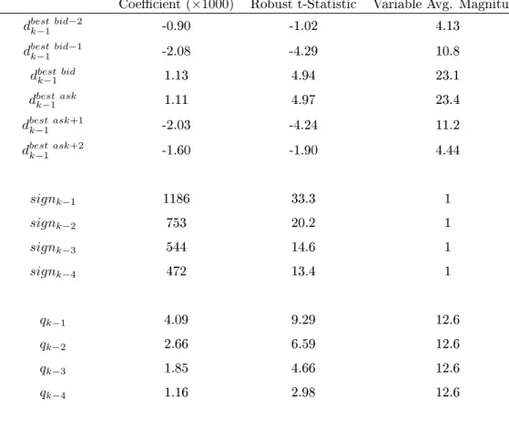
section 4.3.1. Specically, I regressykon the changes in resting depth between aggressive ordersk−1
andkat each of the six price levels within two ticks of the best bid or best ask, the signs of aggressive
ordersk−1throughk−4, and the signed executed quantities of aggressive ordersk−1throughk−4.
For symmetry, I adopt the convention that sell depth is negative and buy depth is positive, so that an increase in buy depth has the same sign as a decrease in sell depth. Denoting the row vector of
the 14 regressors byzk−1, and a column vector of 14 coecients byΓ, I estimate the equation
yk = zk−1Γ +k (13)
The estimated coecients have the expected signs, and their joint signicance is extremely high. I discuss the regression results directly and report coecient estimates in Appendix C.
To compute the excess performance of aggressive orderk, denotedξk, I normalize thekth regression
residual bysignk, the sign of the kth aggressive order:
ξk =signk
yk−zk−1Γˆ
(14)
As discussed in section 4.1, normalizing the cumulative price-changeykby the sign of thekth aggressive
order yields a measure of thekth aggressive order's protability. Likewise, the quantityξk provides a
measure ofkth aggressive order's protability in excess of that expected on the basis of the benchmark
econometric specication. I compute the vectors of direction-normalized residuals separately for each of the 32 trading days in my sample, then combine all of them into a single vector for the entire sample period.
4.3.3 Explained Performance
The price movements predicted by (13) explain a substantial component of the performance of
ag-gressive orders placed by A-HFTs, B-HFTs, and non-HFTs alike.5 Looking ahead, this explanatory
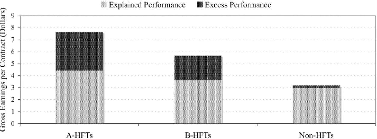
power validates the use of specication (13) as a basis for the more sophisticated analyses in section 5. Figure 1 and Table 1 summarize the overall size-weighted average performance of aggressive orders placed by various trader groups, both in absolute terms, and in excess of the econometric benchmark. Condence intervals are computed via bootstrap.
5Although the variables inzk−1 are all observable before thekth aggressive order arrives, the tted valuezk−1ˆΓis
not literally a forecast ofykin the strictest sense, asΓˆis estimated from data for the entire day. However, the coecient
estimates are extremely stable throughout the sample period, so thinking ofzk−1Γˆas a forecast ofyk is innocuous in
Figure 1. Aggressive Order Performance Relative to Econometric Benchmark 0 1 2 3 4 5 6 7 8 9 A-HFTs B-HFTs Non-HFTs G ros s E arni ngs pe r Cont ra ct (D ol la rs
) Explained Performance Excess Performance
Figure 1: Aggressive Order Performance Relative to Econometric Benchmark
Table 1: Aggressive Order Performance vs. Econometric Benchmark
Mean Mean Absolute Mean Mean Excess Explained
Absolute 99%CI Excess 99%CI Performance
A-HFTs 7.65 (7.54,7.73) 3.22 (3.09,3.36) 57.8%
B-HFTs 5.67 (5.57,5.77) 2.04 (1.90,2.17) 64.0%
Non-HFTs 3.19 (3.12,3.26) 0.22 (0.14,0.29) 93.06%
Although the unexplained component of the A-HFTs' performance is large in absolute terms, and massive relative that of the B-HFTs and the non-HFTs, the econometric controls in (13) nevertheless explain more than half of the A-HFTs' performance on their aggressive orders. The exploratory trading model developed earlier assumed that A-HFTs ultimately traded ahead of easily predictable demand innovations (when liquidity conditions were suitably unaccommodating), and the explanatory power of the econometric benchmark for the A-HFTs' performance substantiates this assumption.
4.4 A-HFTs' Losses on Small Aggressive Orders
The A-HFTs' aggressive orders tend to become more protable as order-size increases.6 In fact, despite
earning money from their aggressive orders on average, the A-HFTs all tend to lose money on the smallest aggressive orders that they place. Note also that I refer here to the size of the aggressive orders A-HFTs submit, not the quantity that executes, so the small orders were intentionally chosen to be small, and the large orders intentionally chosen to be large.
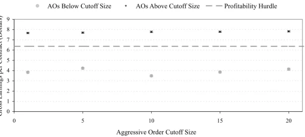
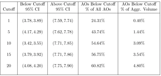
To make precise both the meaning of small aggressive orders, and A-HFTs' losses on them, I specify cutos for order-size and compute the average performance of A-HFTs' aggressive orders below and above those size cutos. Figure 2 and Table 2 display bootstrap condence intervals for the executed-quantity-weighted average performance of A-HFTs' aggressive orders weakly below and
strictly above various order-size cutos.Figure 2. A-HFT Performance on Small and Larger Aggressive Orders (95% Conf. Intervals)
0 1 2 3 4 5 6 7 8 9 0 5 10 15 20
Aggressive Order Cutoff Size
G ros s E arni ngs pe r Cont ra ct (D ol la rs )
AOs Below Cutoff Size AOs Above Cutoff Size Profitability Hurdle
Figure 2: A-HFT Performance on Small and Larger Aggressive Orders (95% Conf. Intervals) 6This eect appears whether price-changes are measured between the respective last prices at which successive
aggressive orders execute (correcting for bid-ask bounce), or between the respective rst prices at which they execute, so the positive relationship between executed quantity and subsequent favorable price movements is not simply an artifact of large orders that eat through one or more levels of the orderbook.
Table 2: Performance of A-HFTs' Aggressive Orders (Dollars per Contract)
Below Cuto Above Cuto AOs Below Cuto AOs Below Cuto
Cuto 95%CI 95%CI % of All AOs % of Aggr. Volume
1 (3.78,3.89) (7.59,7.74) 24.31% 0.40% 5 (4.17,4.29) (7.62,7.78) 43.74% 1.44% 10 (3.42,3.55) (7.71,7.85) 54.64% 3.09% 15 (3.79,3.92) (7.71,7.86) 56.75% 3.54% 20 (4.08,4.20) (7.75,7.90) 60.82% 4.80%
As shown in Table 2, small aggressive orders represent a substantial fraction of the aggressive orders
that A-HFTs place. A given A-HFT places an aggressive order of size20 or less roughly once every
34seconds on average, and this average interval drops to about 3 seconds during periods of intense
market activity. These small orders make up very little of the A-HFTs' total aggressive volume, but
the A-HFTs' losses on them are non-trivial. On average, each A-HFT loses around$7,150per trading
day ($1.8million, annualized) on aggressive orders of size20or less; this loss represents approximately
7.2%of an average A-HFT's daily prots.
There are several reasons why a trader who consistently manages to prot on large aggressive orders might nonetheless place unprotable small aggressive orders, including controlling risk and testing out new strategies. The A-HFTs' diering performance on small and large aggressive orders is also consistent with the pattern that we would expect to see if the small orders were generating valuable information that enabled the A-HFTs to earn greater prots from their large orders, as discussed in section 2. Moreover, the A-HFTs' small aggressive orders could serve several roles at once, so treating them as exploratory would not rule out additional reasons why they might have been placed. Although the A-HFTs' qualitative pattern of losses on small aggressive orders and more-than-osetting gains on larger aggressive orders does not necessarily imply that the A-HFTs engage in exploratory trading, it does suggest that the small orders are at least reasonable candidates for exploratory orders. Identifying candidate exploratory orders provides the starting point for direct tests of the exploratory trading model's sharper empirical predictions.
5 Testing the Exploratory Trading Hypothesis
If the A-HFTs indeed engage in exploration using their small aggressive orders, the exploratory trading model generates the testable predictions presented in section 2.5, which I restate below for convenience: Relative to a benchmark that incorporates the public information about the market response following small aggressive orders placed by anyone, information from the market response following an A-HFT's small aggressive orders:
Predict.1. Explains a significant additional component of that A-HFT's earnings on subse-quent aggressive orders, but
Predict.2. Does not explain any additional component of other traders' earnings on subse-quent aggressive orders, and
Predict.3. Further explains by a significant margin the incidence of that A-HFT's subsequent large aggressive orders
In this section, I consider a simple numeric characterization of the market response following an aggressive order, and I directly test whether the above predictions hold. The rst two predictions concern the explanatory power of market-response information for the performance of subsequent aggressive orders, and I test these two predictions in the same empirical framework. The third prediction, concerning the incidence of large aggressive orders, requires a slightly dierent empirical approach, so I consider this prediction separately. I estimate results for the A-HFTs individually, but for compliance with condentiality protocols, I present cross-sectional averages of these estimates.
Empirically, these average results are representative of the results for individual A-HFTs.7
5.0.1 A Simple Measure of Market Response
Dene an aggressive order to be small if that order's submitted size is less than or equal to a specied
size parameter, which I will denote byq¯.
I characterize the market response to a small aggressive order using subsequent changes in order-book depth. I examine the interval starting immediately after the arrival of a given small aggressive order and ending immediately before the arrival of the next aggressive order (which may or may not 7Throughout the E-mini market, there exist assorted linkages between various trading accounts (as, for example, in
the simple case where single rm trades with multiple accounts), so the trading-account divisions do not necessarily deliver appropriate atomic A-HFT units. Though the specics are condential, the appropriate partition of the A-HFTs is entirely obvious. For brevity, I use individual A-HFT as shorthand to individual atomic A-HFT unit, as applicable.
be small), and I sum the changes in depth at the best bid and best ask that occur during this interval. As in section 4.3, I treat sell depth as negative and buy depth as positive. I also normalize these depth changes by the sign of the preceding small aggressive order to standardize across buy orders and sell orders.
To simplify the analysis and stack the odds against nding signicant results, I initially focus only on the signs of the direction-normalized depth changes. These signs merely indicate whether or not resting depth moved further in the direction of the preceding small aggressive order. For a given value
ofq¯, I construct the indicator variableΩ, withkth elementΩk dened by
Ωk = 1 if DC(k;any,q¯)>0 0 otherwise (15)
whereDC(k;any,q¯)denotes the direction-normalized depth change following the last small aggressive
order (submitted by anyone) that arrived before thekth aggressive order. Similarly, I construct the
indicator variableΩA, withkth elementΩA
k dened by ΩAk = 1 if DC(k;AHF T,q¯)>0 0 otherwise (16)
where DC(k;AHF T,q¯) denotes the direction-normalized depth change following the last small
ag-gressive order submitted by a specied A-HFT that arrived before thekth aggressive order.
5.1 Performance of Aggressive Orders
5.1.1 Empirical Strategy: OverviewThough the implementation is slightly involved, my basic empirical strategy is straight-forward. First, I augment the benchmark regression from section 4.3 using either:
1. Market response information from the last small aggressive order placed by anyonei.e.,Ω, or
2. Both market response information from the last small aggressive order placed by anyone, and market response information from the last small aggressive order placed by a specied
After estimating both of the specications above, I nd the additional component of performance on larger aggressive orders explained by the second one relative to the rst. The market response following an arbitrary small aggressive order is publicly observable. However, because the E-mini market operates anonymously, the distinction between a small aggressive order placed by a particular A-HFT and an arbitrary small aggressive order is private information, available only to the A-HFT who placed the order. Because the market response information from the last small aggressive order placed by anyone is weakly more recent than the market response information from last small aggressive order placed by the A-HFT, comparing the second specication above to the rst helps to isolate the eects attributable to private information from eects attributable to public information.
Finally, I compare the additional explained performance for the specied A-HFT to the additional explained performance for all other traders. Intuitively, we want to verify that the A-HFT's ex-ploratory information provides extra explanatory power for the subsequent performance of the trader privy to that information (the A-HFT), but not for the performance of traders who aren't privy to it (everyone else). Note that everyone else includes the A-HFTs other than the specied A-HFT. Some A-HFT accounts and B-HFT/non-HFT accounts belong to the same rms, and various B-HFTs/non-HFTs may be either directly informed or able to make educated inferences about what one or more A-HFTs do. As a result, we should not necessarily expect exploratory information generated by an A-HFT's small orders to provide no explanatory power whatsoever for all other traders' performance. However, we should still expect the additional explanatory power for the A-HFT's performance to signicantly exceed that for the other traders' performance.
Controlling for Public Information Comparing the second specication to the rst one controls for the eects of most public information, but there could conceivably be some public information that is correlated with the market response to a specied A-HFT's small aggressive orders and yet uncorrelated with the market response to small aggressive orders placed by everyone else. A natural way to handle this concern is to compare the additional explained performance for the specied A-HFT to the additional explained performance for some other traders who use the same public information. Although trading objectives and sophistication vary widely across many participants in the E-mini market, all of the HFTs are sophisticated, protable traders, with similar (very short) investment horizons, so it is extremely plausible that they all use very similar public data. Comparing the additional explained performance for the specied A-HFT to that for the other HFTs therefore serves
as an added control for any lingering eects from public information. 5.1.2 Estimation Procedure
In the model of exploratory trading presented earlier, exploratory information was valuable only in conjunction with information about future aggressive order ow. Following this notion, I incorporate
market-response information by using the indicatorsΩandΩAto partition the benchmark regression
from section 4.3.
Recall that in section 4.3, I estimated equation (13),
yk = zk−1Γ +k
whereyk denoted the cumulative price-change between the aggressive orders k and k+ 50, and the
vectorzk−1 consisted of changes in resting depth between aggressive orders k−1 andk, as well as
the signs and signed executed quantities of aggressive ordersk−1throughk−4. Using the indicator
Ω, I now partition the equation above into two pieces and estimate the equation
yk = Ωkzk−1Γa+ (1−Ωk)zk−1Γb+k (17)
Next, I use the indicatorΩA to further partition (17), and I estimate the equation
yk = ΩAk (k) Ωkzk−1Γc+ (1−Ωk)zk−1Γd
+ (18)
1−ΩAk
Ωkzk−1Γe+ (1−Ωk)zk−1Γf+k
The variables yk and zk−1 denote the same quantities as before, and the Γj terms each represent
vectors of 14 coecients.
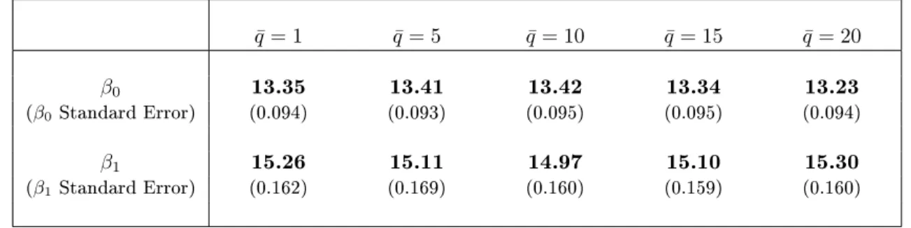
I estimate (17) and (18) for q¯= 1,5,10,15,20, and for each specication I calculate the relative
excess performance of the specied A-HFT, and of all other trading accounts, on aggressive orders
of size strictly greater thanq¯. As in section 4.3, I compute the performance of aggressive orderk in
excess of that explained by each regression by normalizing thekth residual from the regression by
the sign of thekth aggressive order. I now also control for order-size eects directly by regressing the
direction-normalized residuals (for the orders of size strictly greater thanq¯) on the (unsigned) executed
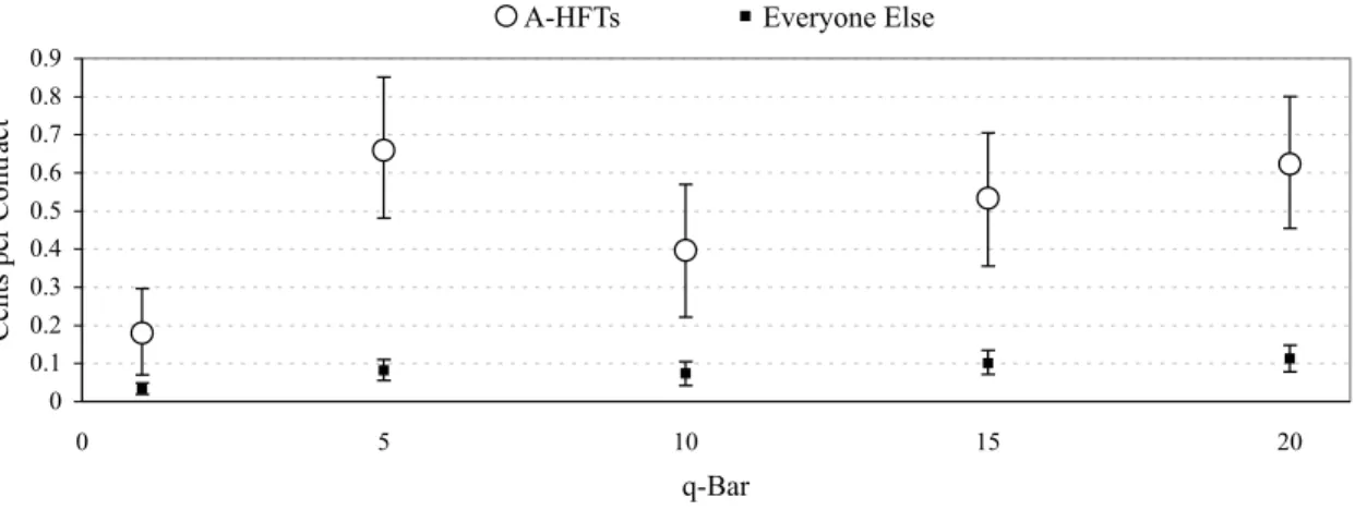
![Figure 4. [A-HFT Addt'l Explained] - [Everyone Else Addt'l Explained] (95% Conf. Intervals) 00.10.20.30.40.50.60.70.8 0 5 10 15 20 q-Bar](https://thumb-us.123doks.com/thumbv2/123dok_us/9810774.2866856/33.918.139.773.150.341/figure-hft-addt-explained-addt-explained-conf-intervals.webp)
![Figure 5. [A-HFT Addt'l Explained] - [Other HFTs Addt'l Explained] (95% Conf. Intervals) -0.100.10.20.30.40.50.60.7 0 5 10 15 20 q-Bar](https://thumb-us.123doks.com/thumbv2/123dok_us/9810774.2866856/34.918.144.765.146.348/figure-addt-explained-other-hfts-addt-explained-intervals.webp)